Application of Computational Intelligence Methods in Agricultural Soil–Machine Interaction: A Review

Abstract

Rapid advancements in technology, particularly in soil tools and agricultural machinery, have led to the proliferation of mechanized agriculture. The interaction between such tools/machines and soil is a complex, dynamic process. The modeling of this interactive process is essential for reducing energy requirements, excessive soil pulverization, and soil compaction, thereby leading to sustainable crop production. Traditional methods that rely on simplistic physics-based models are not often the best approach. Computational intelligence-based approaches are an attractive alternative to traditional methods. These methods are highly versatile, can handle various forms of data, and are adaptive in nature. Recent years have witnessed a surge in adapting such methods in all domains of engineering, including agriculture. These applications leverage not only classical computational intelligence methods, but also emergent ones, such as deep learning. Although classical methods have routinely been applied to the soil–machine interaction studies, the field is yet to harness the more recent developments in computational intelligence. The purpose of this review article is twofold. Firstly, it provides an in-depth description of classical computational intelligence methods, including their underlying theoretical basis, along with a survey of their use in soil–machine interaction research. Hence, it serves as a concise and systematic reference for practicing engineers as well as researchers in this field. Next, this article provides an outline of various emergent methods in computational intelligence, with the aim of introducing state-of-the-art methods to the interested reader and motivating their application in soil–machine interaction research.

1. Introduction

Soil-engaging tools or machines are an indispensable part of mechanized agriculture. A soil–machine interaction deals with a behavior of tools or machines with soil that results in either tillage, traction, or compaction. The soil–machine interaction is mainly categorized into tillage, traction, and compaction [1]. In traction, a powered traction element (wheel/track) of the vehicle operates on deformable soil, causing soil shear to generate the traction [2]. The soil-derived traction force overcomes the vehicle’s resisting forces and maintains its constant motion with its slip and terrain damage [3]. The slip is a principal form of vehicle power loss and one of the prime reasons behind the off-road vehicle’s worst traction efficiency. Tractors are the prime movers in agriculture and are mainly used for drawbar work. The drawbar is the most used but the least efficient power outlet, and approx. 20 to 55% of the tractor’s available energy is wasted at the soil-tire interface, often resulting in soil compaction and tire wear [4]. Therefore, the traction performance of the vehicle is quantified in terms of traction, slip, and power efficiencies on certain terrain. In the off-road vehicle, it is critical to optimize or increase the working capacity, efficiency, and reduce slip and terrain damage. Multiple variables, such as traction element geometry, operating variables, and soil physical conditions, influence vehicle traction performance. Therefore, traction models are often proposed to optimize off-road vehicle performance (e.g., drawbar, slip, traction efficiency).

Tillage alters the soil mechanically to create favorable conditions for crops [2]. It employs either powered or unpowered mechanical devices (tool/implement) to apply forces to the soil, resulting in soil cutting, inversion, pulverization, displacement, mixing, or a collective action aiming to obtain desired conditions [5]. Most tillage devices are passive (unpowered), known as conventional tillage, where a drawbar is applied to the device, and its movement through soil results in tillage. In contrast, active tillage, also known as rotary tillage, employs a powered device to transmit power to the soil. The powered tool comparatively moves greater soil volume than required, and energy cost increases with a working width and depth. Tillage is the most energy-intensive agricultural operation and accounts for nearly half of the total crop production energy [6].

Tillage energy is influenced by multiple factors, including soil conditions (initial condition, texture, bulk density, moisture content, and crop residue cover), tool parameters (shape, size, and cutting-edge sharpness), and operating parameters (depth and speed) [5,6]. Therefore, extensive literature is available that aims to reduce tillage input energy by optimizing those factors. The research efforts mainly revolved around the soil failure pattern, soil movement, and force or energy prediction models [5,6]. The information on tillage force or energy is critical to select tillage types, tools, control variables, energy management, optimization, and reducing excessive soil pulverization. For example, knowing the tool draft in specific soil helps select the tractor size with a matching implement, reducing operation costs and negative soil impacts. Therefore, tillage force or energy prediction models are necessary from an energy optimization perspective.

Soil compaction is a leading factor in degrading productive farmland [7,8]. It has degraded an estimated 83 Mha of farmland [7,9] and affected around 45% of agrarian soil [10,11]. Natural and artificial activities are responsible for soil compaction. The artificial activities involved in crop production can severely affect soil compaction. These activities include heavyweight machinery, and its intense use, uncontrolled vehicle traffic, multiple passes, operating machines under unfavorable conditions (e.g., wet soil), repeated tillage, and bad crop rotation [7,12,13]. In addition to topsoil compaction, a subsoil or plow pan is caused by heavy vehicular movement, heavy plow weight, downward forces from a plow bottom/disk, and repeated tillage. Soil compaction resulting from the soil–machine interaction influences the soil structure, porosity, permeability, and density [7,14], which impacts the crop yield and may degrade the soil. The soil compaction evolved from soil-machine interaction is a complex process that involves multiple interrelated factors. Hence, optimizing the vehicle parameters (e.g., tire type, orientation, inflation pressure, axle weight, traffic), tillage parameters (tool shape, weight, depth, speed, and tillage intensity), and assessing the initial field conditions (soil moisture) can minimize or eliminate the soil compaction.

The soil–machine interaction is a dynamic and intricate process that includes multivariate. However, understanding and accurately describing (models) the soil–machine interaction may provide a solution to sustainable agricultural production. For example, a slight improvement in the tillage tool design or practice could significantly reduce the input energy and avoid excessive soil pulverization or compaction. Likewise, improving the vehicle traction efficiency may increase the working capacity, save energy, and avoid terrain damage or compaction.

In recent years, computational intelligence (CI) methods have succeeded in solving intricate problems in agriculture and life science. The literature shows that researchers, scholars, and engineers have implemented cutting-edge CI methods, including neural networks, fuzzy logic, neuro-fuzzy systems, support vector machines, and genetic algorithms, to solve a challenging problem in the soil tillage and traction domain. However, it lacks a comprehensive, curated source of reference and a detailed and well-organized discussion on the application of CI methods on the soil–machine interaction. Therefore, this study aimed to survey and analyze the recent research efforts in the soil–machine interaction and critically review the existing methods with a detailed discussion. The article provides brief information, progress, and future direction on CI methods in the soil tillage and traction domain. The proposed study would serve as a concise reference to the reader, engineers, researchers, and farm managers who are further interested in the soil–machine interaction. It is also a quick and systematic way to understand the applicable methods that allow crucial decision-making in farm management.

The review is organized into the following sections: Section 2 discusses the traditional approach used in soil–machine interaction modeling. It also discusses the strengths and limitations of the traditional approach. Section 3 presents a brief overview of popular CI methods, while Section 4 discusses the popular CI methods. These sections provide a piece of fundamental and in-depth information to the readers. Section 5 provides a brief literature survey on CI methods that are employed in soil–machine interaction studies. It also contains the followed literature survey methodology. In Section 6, the strengths and limitations of CI methods were identified. Section 7 talks about the other emergent CI models that may provide a better solution than popular CI methods. Section 8 discusses the significance, scope, and future direction.

2. Traditional Modeling Methods

In recent decades, numerous methods have been proposed to evaluate, analyze, model, and understand the soil–machine interaction, which aims to optimize energy, time, efficiency, and machine or tool service life with reduced wear. The methods are explained as follows:

2.1. Analytical Method

Analytical methods are based on physical principles of soil/terrain, machine parameters, and simple assumptions. The traction force is often computed from a soil–tire contact–surface interface and stress distribution (shear and normal) [5,15]. However, both soil and tire deform during the process, making it challenging to describe in mathematical terms. Moreover, machine dynamics, varying soil conditions, its elastic-plastic nature, and inadequate information on boundary conditions make the soil–machine interaction a very complex problem to model accurately. These challenges raise questions on its adaptability [3,5,15,16].

Likewise, in tillage, soil resistance is computed with a logarithmic spiral method and passive earth pressure theory [6]. These are assumption-based methods that do not include the actual soil failure patterns that vary with tool parameters (shape, rake angle, speed) and soil parameters (moisture, density, and structure) [17,18,19,20]. Moreover, the analytical methods are suitable for simple shapes, but difficult for the complex shape tool [5,6]. Thus, it exhibits limited applicability for tool design and energy or force prediction.

2.2. Empirical Method

Empirical methods are derived from a large amount of experimental data, where the best-fit regression curve explains a relationship among the selected variables. Empirical equations are simple and consist of a few variables with constants specific to the soil, track/wheel, tool type, machine configuration, and operating conditions. Thus, these equations cannot be extrapolated to the other problems, restricting their broad applicability [3,5,15]. Thus, precautions are necessary on a new tire, tillage tool, and test environment [3,5]. Moreover, it requires a large amount of experimental data, which is laborious and costly. Additionally, it is subjected to a multi-collinearity problem, arising from not truly dependent factors [21].

2.3. Semi-Empirical Method

Semi-empirical method combines experimental data, empirical formulations, and analytical methods. In traction studies, the stress (normal and shear) and soil deformation are computed by assuming stress under a flat plate, and bevameter is used [3,5,15]. The flat plate is non-flexible, but the tire or track is flexible, working on deformable soil. Thus, this method requires improvement. Similarly, a passive earth pressure theory explains the soil-failure pattern for a simple shaped tillage tool [5,6,19]. However, adopting the earth pressure theory to other complex shaped tools is challenging [5,17,22,23]. Semi-empirical is a hybrid, reliable, and the most common method, although equations derived from assumptions limit its accuracy in varying terrain.

2.4. Numerical Method

Numerical methods such as finite element and discrete element were extensively studied, and lately in soil tillage and traction domain [3,5,15,19,24,25,26,27,28]. The detailed examples can be found here [25,26]. These methods have successfully modeled the complex, dynamic, and non-linear soil–machine interaction problems with greater accuracy and fewer assumptions [3,25,26]. However, it is a highly computational method consisting of a virtual simulation with commercial software installed on a high-speed computer. Therefore, it is time-consuming and requires special and costly resources. Moreover, the simulation setup needs an accurate description of a soil medium that varies on a spatial-temporal basis, making it challenging.

In short, the traditional modeling methods have a few limitations and are very specific to machine or tool types and experimental conditions, which restricts their wide applicability.

3. Computational Intelligence: An Overview

Broadly speaking, the term “computational intelligence” refers to a wide class of approaches that rely on approximate information to solve complex problems [29,30,31,32]. There are a vast array of such problems (e.g., classification, regression, clustering, anomaly detection, function optimization), where CI models have been extensively used. In the available literature on soil–machine interactions, these models have been used for regression tasks. Accordingly, this article describes CI models from a regression standpoint. However, as some articles have used CI optimization approaches for training the models (i.e., model parameter optimization for best performance), CI-based optimization algorithms are also addressed here, albeit in the context of training.

Many CI models are derived from paradigms observed in the natural world. Artificial neural networks (NN), deep neural networks (DNN), and radial basis function networks (RBFN) are structures that loosely resemble the organization of neurons in higher animals. Fuzzy inference systems (FIS) perform computations in a manner analogous to verbal reasoning. Adaptive neuro-fuzzy systems (ANFIS) are designed to combine the attractive features of NN and FIS. These models are very well suited for regression tasks.

Other CI regression models, which are designed from purely mathematical considerations, do not have any natural counterparts. This class of machine learning methods includes support vector regression (SVR) and Bayesian methods.

Natural phenomena also provide the backdrop of CI optimization methods. Genetic algorithms (GA) are modeled after Darwinian evolution, while particle swarm optimization (PSO) simulates the foraging strategy of a swarm of organisms. These methods have been routinely used to train other CI models [33,34,35,36].

CI models for regression are data-driven approaches. In soil–machine interaction studies, the data are typically collected from field experiments. Each sample in the data is a pair $\left(\mathbf{x}\left(n\right),\mathbf{t}\left(n\right)\right)$, where n is a sample index. The quantity $\mathbf{x}\left(n\right)\in {\mathbb{R}}^M$ in a sample is an M-dimensional input, $\mathbf{t}\left(n\right)\in {\mathbb{R}}^N$ is its corresponding M-dimensional target (or desired output) vector. The symbol $\Theta$ is used in this article to denote the set of all trainable parameters of any CI model. Wherever necessary, it may be treated as a vector. Note that throughout this article, italicized fonts are used to represent scalar quantities, and bold fonts for vectors (lowercase) and multi-dimensional arrays (uppercase).

3.1. Data Preprocessing

Preprocessing is often essential before using data to train a CI model. It renders the data more suitable for CI models.

(i)

Data Normalization: This is the most rudimentary form of preprocessing. Each field of the data are normalized separately so that the entries lie in some desired range, usually $[0,1]$ or $[-1,1]$.

(ii)

Data Cleaning: Experimental data may contain some missing entries. One option to deal with the issue is to remove every sample, which contains a missing (scalar) field. This practice may be wasteful, particularly when the data are limited. If so, missing fields may be filled with means, medians, or interpolated values. Corrupted entries can also be treated in this manner [37]. Noise reduction is another form of data cleaning. When the noise follows a non-skewed distribution around a zero mean, noise removal may not be necessary in regression tasks. Convolution with Gaussian or other filters is a common filtering tool for time series data [38].

(iii)

Dimension Reduction: Dimension reduction is useful when the number of input dimensions, say $M^{\prime }$ is too high. Principal component analysis (PCA) is widely used for this purpose. More advanced techniques for dimension reduction include nonlinear PCA [39] and independent component analysis (ICA) [40].

(iv)

Spectral Transformation: This technique can be used with periodic data. The classical Fourier transform is regularly used to extract frequency components of such data; it does not preserve the time information of the input. Wavelet transforms can be used when the data must incorporate frequency and temporal components.

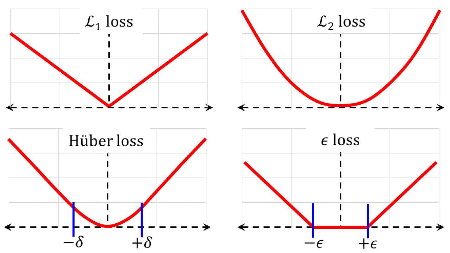
The samples are randomly divided into three disjoint sets—the training set ${\mathcal{S}}_t$, the test set ${\mathcal{S}}_s$, and the validation set ${\mathcal{S}}_v$. Training samples are used directly to adjust the model parameters in small increments. Unlike them, samples in ${\mathcal{S}}_s$, are not used explicitly to compute parameter increments. Instead, testing samples are used intermittently during training to monitor progress. Validation samples in ${\mathcal{S}}_v$ are used as surrogates for the real world. The performance of the CI model is evaluated with respect to ${\mathcal{S}}_v$ only after training is completely accomplished. Approximately 60%–80% of the samples are assigned to ${\mathcal{S}}_t$ and the remainder divided roughly equally between ${\mathcal{S}}_s$ and ${\mathcal{S}}_v$.

3.2. Loss Functions

The purpose of training any model is to minimize the differences between the targets and the true outputs, quantified in terms of its loss [41,42], which is the average of the penalties incurred by all samples. The symbol $\mathcal{L}$ is used to represent the loss. The model’s loss with respect to samples in the dataset $\mathcal{S}$ is,

$${\mathcal{L}}_{\Theta }\left(\mathcal{S}\right)=\frac{1}{\left|\mathcal{S}\right|}\sum _{n\in \mathcal{S}}l\left(t\right(n)-y(n\left)\right)$$

(1)

The optional subscript $\Theta$ in Equation (1) above is used to highlight the loss’s dependence on the model parameters. Each term $l(·)$ is a sample penalty or error. Using this convention, ${\mathcal{L}}_{\Theta }\left({\mathcal{S}}_t\right)$, ${\mathcal{L}}_{\Theta }\left({\mathcal{S}}_s\right)$, and ${\mathcal{L}}_{\Theta }\left({\mathcal{S}}_v\right)$ are the training and validation losses.

Several loss functions have been proposed. The following are the most commonly used.

(i)

Mean squared (${\mathcal{L}}_2$) loss: For scalars, this loss is the average of the squared differences between the network’s outputs $y\left(n\right)$, for inputs $\mathbf{x}\left(n\right)$ and the corresponding targets, so that, ${\mathcal{L}}_2={\left|\mathcal{S}\right|}^{-1}{\sum }_n{[y\left(n\right)-t\left(n\right)]}^2$. For vector outputs, the Euclidean norm $\left|\right|\mathbf{y}\left(n\right)-\mathbf{t}\left(n\right)\left|\right|$ is used, where $\mathbf{y}\left(n\right)$ is the model’s vector output. The ${\mathcal{L}}_2$ loss is the most commonly used function. Using quadratic penalty terms makes the function quite sensitive to statistical outliers.

(ii)

Averaged absolute (${\mathcal{L}}_1$) loss: This is the average of the absolute difference, ${\mathcal{L}}_1={\left|\mathcal{S}\right|}^{-1}{\sum }_n|y\left(n\right)-t\left(n\right)|$. The ${\mathcal{L}}_1$ loss is used to avoid assigning excessive penalties to noisier samples. On the other hand, its effectiveness is compromised for data with copious noise.

(iii)

Hüber loss: The Hüber loss represents a trade-off between the ${\mathcal{L}}_2$ and ${\mathcal{L}}_1$ losses [43]. Samples where the absolute difference is less than a threshold $\delta$ incur a quadratic penalty, while the remaining ones have a linear penalty. It is obtained as the average ${\left|\mathcal{S}\right|}^{-1}{\sum }_n{l}_{\delta }\left(n\right)$, where $l_{\delta }\left(n\right)$ is the penalty of the n^th sample,

$$l_{\delta }\left(n\right)=\left\{\begin{array}{cc}\frac{1}{2}{[y\left(n\right)-t\left(n\right)]}^2,\hfill & \mathrm{if}\left|y\right(n)-t(n\left)\right|<\delta ;\hfill \\ \delta |y\left(n\right)-t\left(n\right)|-\frac{1}{2}{\delta }^2,\hfill & \mathrm{otherwise}.\hfill \end{array}\right.$$

(2)

As the Hüber loss function is not twice differentiable at $\pm \delta$, the similarly shaped log-cosh function below can be used in its place,

$$l_{lc}\left(n\right)={\log }_e\frac{1}{2}\left(e^{y\left(n\right)-t\left(n\right)}+e^{t\left(n\right)-y\left(n\right)}\right).$$

(3)

(iv)

$ϵ$-Loss: This loss does not apply a penalty when the difference $y\left(n\right)-t\left(n\right)$ lies within a tolerable range $[-ϵ,+ϵ]$, for some constant $ϵ$. A linear penalty is incurred whenever the numerical difference lies outside this range. In other words, ${\mathcal{L}}_{ϵ}={\left|\mathcal{S}\right|}^{-1}{\sum }_n{l}_{ϵ}\left(n\right)$, where,

$$l_{ϵ}\left(n\right)=\left\{\begin{array}{cc}0,\hfill & \mathrm{if}\left|y\right(n)-t(n\left)\right|<ϵ;\hfill \\ \left|y\right(n)-t(n\left)\right|-ϵ,\hfill & \mathrm{otherwise}.\hfill \end{array}\right.$$

(4)

Since the loss function is not differentiable at $\pm ϵ$, if needed, a subgradient in $[0,1]$ can be used as a substitute for its derivative at $\pm ϵ$.

The shapes of the above loss functions are illustrated in Figure 1. The log-cosh loss, which is similar to the Hüber loss, is not shown. There are several other loss functions, including those that are specific to the application, that have not been listed here.

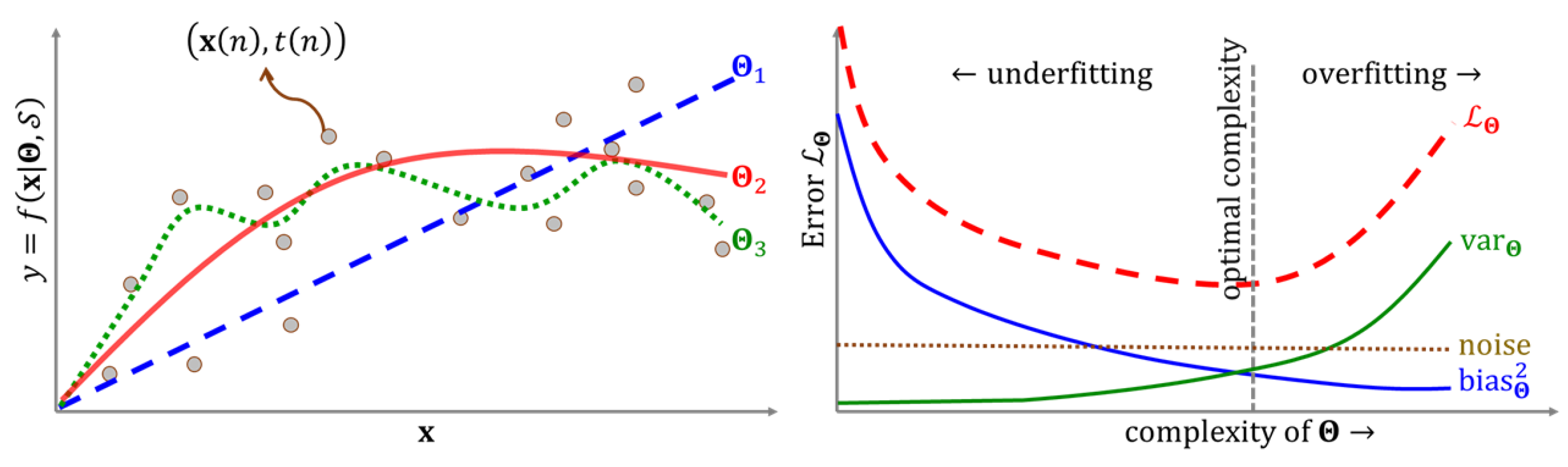
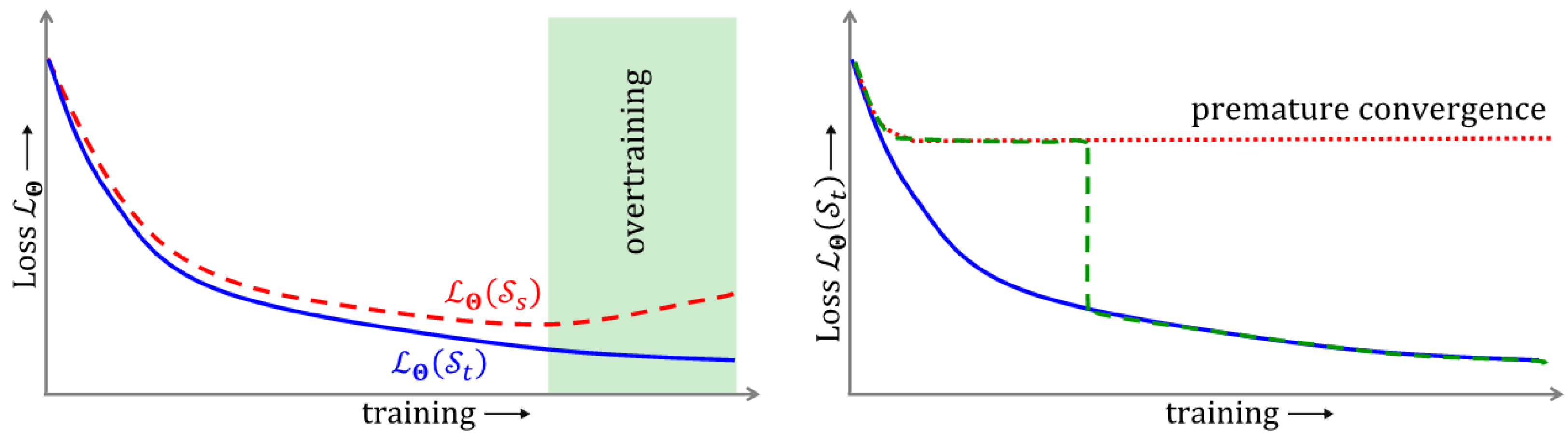
3.3. Model Selection

Model complexity is a key concept in statistical learning theory, closely related to overfitting. The complexity of a model can be quantified as the number of independent scalar parameters used to compute its output and their ranges. The V-C (Vapnik–Chervonenkis) dimensionality of a model is one such measure of complexity [44] that has led to the development of support vector machines.

Model complexity is a critical factor that should be considered during model selection. Low-complexity models tend to exhibit a bias towards specific input-output maps. For instance, a linear model, which is the least complex regression model, cannot be used to capture nonlinear input–output relationships. Conversely, increasing a CI model’s complexity endows it with more degrees of freedom to fit the training data. Due to its lower bias, training the model yields significantly lower training error ${\mathcal{L}}_{\Theta }\left({\mathcal{S}}_t\right)$. Unfortunately, a model with too large a complexity becomes too sensitive to extraneous artifacts present in its training dataset ${\mathcal{S}}_t$, such as random noise, sampling, or aliasing. These are extraneous artifacts that do not reflect any underlying input–output relationship. As stated in another manner, as the model’s complexity increases, so do its variance. The model with higher variance performs poorly in the real world, with inputs outside ${\mathcal{S}}_t$. This is reflected in terms of its higher validation loss ${\mathcal{L}}_{\Theta }\left({\mathcal{S}}_v\right)$. In general, the model’s effective loss can be decomposed into three components,

$${\mathcal{L}}_{\Theta }={\mathrm{bias}}_{\Theta }^2+{\mathrm{var}}_{\Theta }+\mathrm{noise}.$$

(5)

The square of the bias term is used in (5), as it can acquire positive and negative values. The noise component is an artifact introduced by the external environment, and is independent of the model $\Theta$. Selecting a CI model with the optimal complexity is a well-known bias-variance dilemma in machine learning. This phenomenon is depicted in Figure 2.

A widely used approach to keep the model’s complexity at lower levels is by adding a regularization term $\mathcal{R}(·)$ to the loss function. Regularizers are routinely devised in terms of the model parameters in $\Theta$. If $\Theta$ is treated as a vector of parameters, $\mathcal{R}(\Theta )={\left|\right|\Theta \left|\right|}_1$ and $\mathcal{R}(\Theta )={\left|\right|\Theta \left|\right|}_2^2$ are used as LASSO (least absolute shrinkage and selection operator) and ridge regularizers. The elastic net function, which is the convex combination of the LASSO and ridge terms, so that $\mathcal{R}(\Theta )={r\left|\right|\Theta \left|\right|}_2^2+{(1-r)\left|\right|\Theta \left|\right|}_1$ (where $0<r<1$ is a constant), is another popular choice for regularization [45].

3.4. Training Algorithms

At present, almost all training algorithms rely on the basic gradient descent. If ${\mathcal{L}}_{\Theta }(·)$ is the loss function (which may include a regularization term), the parameters of the model are incremented using the training samples in ${\mathcal{S}}_t$, as shown in the following expression,

$$\Theta \leftarrow \Theta +\eta {\nabla }_{\Theta }{\mathcal{L}}_{\Theta }\left({\mathcal{S}}_t\right)$$

(6)

The quantity $\eta$ in the above expression is the gradient descent step size, commonly referred to as the learning rate in CI terminology. The operator ${\nabla }_{\Theta }$ is the gradient (vector derivative) w.r.t. $\Theta$.

Since the loss ${\mathcal{L}}_{\Theta }\left({\mathcal{S}}_t\right)$ is the sum of all sample penalties $l\left(n\right)$, where $n\in {\mathcal{S}}_t$, a direct implementation of Equation (6) would require a pass over all samples in ${\mathcal{S}}_t$ before $\Theta$ can be updated. As this is computationally burdensome (particularly for large datasets), training algorithms invariably use stochastic gradient descent (SGD). Before every training epoch of SGD, the samples in ${\mathcal{S}}_t$ are rearranged randomly. The vector parameter $\Theta$ is incremented once for each sample n, using the gradient ${\nabla }_{\Theta }l\left(n\right)$.

In theory, SGD can lead to a speed up the training algorithm by a factor $|{\mathcal{S}}_t|$. However, as the directions of the gradients ${\nabla }_{\Theta }l\left(n\right)$ are not perfectly aligned with one another, the actual speed up is considerably less than $|{\mathcal{S}}_t|$. Adding a momentum term to the gradient step helps alleviate this situation. If in step $n-1$ the parameter $\Theta$ is incremented by an amount $\Delta \Theta (n-1)$, in the next step n, the increment would be $\Delta \Theta \left(n\right)=\eta {\nabla }_{\Theta }l\left(n\right)+\mu \Delta \Theta (n-1)$. The quantity $\mu$ ($0\le \mu <\eta$) is the momentum rate.

The convergence rate of the training algorithm can be significantly improved by Newton’s algorithm, which requires the Hessian matrix ${\nabla }_{\Theta }^2$. It can be readily established that the outer product ${\nabla }_{\Theta }{\nabla }_{\Theta }^{\mathrm{T}}$ is a close approximation of the Hessian. In the Levenberg-Marquardt algorithm [46], the diagonal elements of this matrix are incremented by an amount $\mu$ to improve the conditioning. Accordingly, incremental updates with the Levenberg-Marquardt algorithm are implemented as per the following rule,

$$\Theta \leftarrow \Theta +{({\nabla }_{\Theta }{\nabla }_{\Theta }^{\mathrm{T}}+\mu \mathbf{I})}^{-1}{\nabla }_{\Theta }{\mathcal{L}}_{\Theta }\left({\mathcal{S}}_t\right)$$

(7)

Overtraining—a problem that is closely related to overfitting, is frequently encountered during training. This is shown in Figure 3. Since samples in ${\mathcal{S}}_t$ are used to compute the gradient, as long as $\eta$ is small enough, the training loss decreases each time the parameters are incremented. Initially, the test loss $\mathcal{L}\left({\mathcal{S}}_t\right)$ also drops with training. However, after the model has undergone a significant amount of training, $\mathcal{L}\left({\mathcal{S}}_t\right)$ begins to rise. Applying (6) further will cause overtraining.

K-fold cross-validation [47] is an effective means for performance evaluation with sparse data. The samples in ${\mathcal{S}}_t$ are randomly shuffled and split into K groups or folds of equal size. One of the folds is used as the test set ${\mathcal{S}}_s$, and the rest are used to increment $\Theta$. This process is repeated K times, with each fold acting as the test set. The loss averaged over all K folds is a reliable estimate of its true (real-world) loss.

Premature convergence is another issue that is sometimes observed during training (see Figure 3). This occurs if the training algorithm encounters a local minimum of the loss function’s landscape, where the gradient ${\nabla }_{\Theta }$ is very close to zero. Applying (6) or (7) would have little effect on the parameter $\Theta$. A simple method to rectify the situation is to restart the training process from some other (randomly generated) initial point.

The presence of narrow ridges with “V”-shaped cross sections is another reason why the loss may remain unchanged (see Figure 3), giving the appearance of a local minimum for several iterations. Although there is no perceptible drop in the loss, the amount of increment to $\Theta$ is not negligible. Restarts are unnecessary in such situations, for the algorithm eventually leaves such a ridge after multiple updates.

3.5. Optimization Metaheuristics

Existing training algorithms apply optimization metaheuristics, such as GA and PSO, to avoid getting trapped in local minima. These algorithms maintain a set of many candidate solutions, referred to as its population. In each step of the optimization algorithm, a new population is formed out of the existing one, using a variety of stochastic and heuristic search operators. Stochastic operators help the algorithm escape from local minima, while heuristics aid in its convergence towards the global maximum of the objective function.

GAs are useful in training CI regression models. Let the population of such a GA be the set $\left\{{\Theta }^j\right|j=1,2,\cdots \}$, where each $\Theta$ is a candidate model parameter. During each iteration, pairs of solutions are selected from the population in a random manner, but with better ones (in terms of the inverse loss function) being more likely to be picked. Using the crossover operator, a new pair of new solutions is generated from the old ones. For example, in a convex crossover, the existing pair $({\Theta }^i,{\Theta }^j)$ can be used to generate a new pair, $({\Theta }^{i^{\prime }},{\Theta }^{j^{\prime }})=\left(\mu {\Theta }^i+(1-\mu ){\Theta }^j,(1-\mu ){\Theta }^i+\mu {\Theta }^j\right)$.

In the mutation operator, a small amount of perturbation $\Delta {\Theta }^i$ is added to each new candidate parameter so that it becomes equal to ${\Theta }^i+\Delta {\Theta }^i$.

In Gaussian mutation, the perturbation $\Delta {\Theta }^i$ follows a Gaussian distribution centered around the origin. This process is repeated many times until no further improvement can be found.

Although GA and PSO have found widespread use in many optimization applications, their use in machine–soil interaction studies is rather limited. GAs have been used during model training. In these cases, the GA is hybridized with (6) and (7), or any other related method. Gradient descent steps can be incorporated into the GA in different ways. For instance, ${\Theta }^i$ can be mutated into ${\Theta }^i+\Delta {\Theta }^i+\eta {\nabla }_{{\Theta }_i}\mathcal{L}$, where $\Delta {\Theta }^i$ is the random perturbation and ${\nabla }_{\Theta }\mathcal{L}$, the gradient of the training loss $\mathcal{L}$.

Similar hybrid techniques exist for PSO (cf. [48]). However, PSO has not been used in the existing literature on machine–soil interactions. On the other hand, a relatively unknown population-based stochastic algorithm has been used in [49,50].

4. Current Computational Intelligence Models

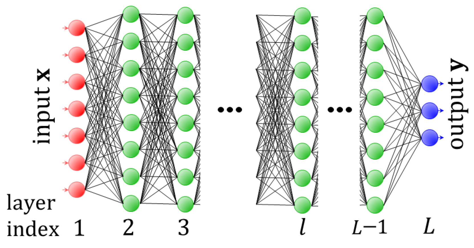
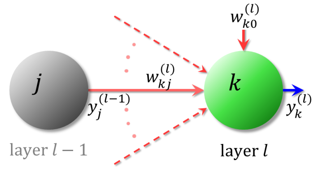
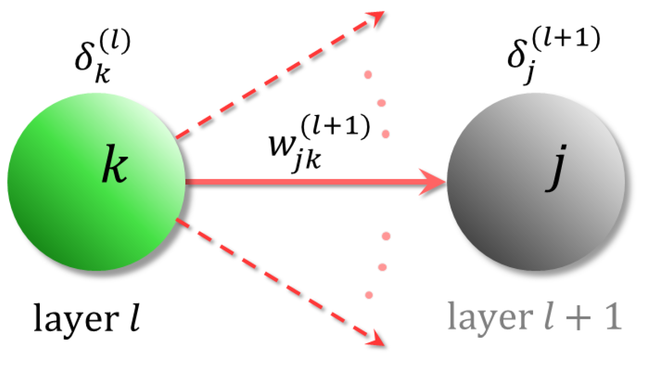
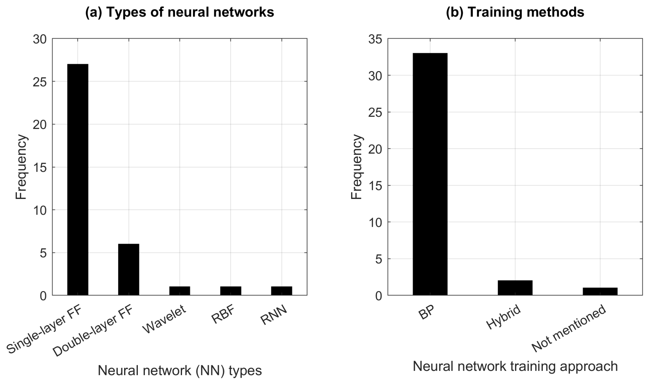
4.1. Neural Networks

Neural network (NN) models have been routinely used in various regression applications since the mid-eighties, wherever a significant amount of data are involved. Neural networks are layered structures consisting of an input layer, one or more intermediate layers, called hidden layers, and an output layer. Each layer comprises elementary processing units or neurons. In a fashion resembling the mammalian cortex, the neurons in each hidden and output layer receive the outputs of those of the preceding layer, as their inputs via weighted synaptic connections.

Figure 4 shows the layout of a neural network with L layers. The indices of the input and output layers are 1 and L, where M and N are the number of neurons in the input and output layers. The vectors $\mathbf{x}$ ($\mathbf{x}\in {\mathbb{R}}^M$) and $\mathbf{y}$ ($\mathbf{y}\in {\mathbb{R}}^N$) denote the network’s input and output.

The size of an NN can be written succinctly as ${\prod }_{l=1}^L{N}^{\left(l\right)}$ where $N^{\left(l\right)}$ is the number of neurons in layer l. For instance, a $3\times 5\times 6\times 2$ NN has three input neurons, a hidden layer with five neurons, another hidden layer with six neurons, and two output neurons. Note that indices of layers (superscripts) are shown within parentheses so as not to confuse them with exponents.

Until recently, NNs were equipped with only one or two hidden layers (so that $L=3$ or $L=4$)—an approach used everywhere in the published literature on soil–machine interaction studies. To distinguish them from deep neural networks (DNNs), which have multiple hidden layers, models with only one hidden layer are referred to as shallow networks. However, for the purpose of this review, networks with two hidden layers are also included in this category. This section focuses on classical methods that are common to both shallow and deep networks. Advanced features that are relevant to DNNs are addressed separately in a subsequent section.

The output of the k^th neuron in a layer indexed l ($l\in \{1\cdots L\}$) is denoted as $y_j^{\left(l\right)}$. Thus, the i^th element of $\mathbf{x}$ is $x_j=y_j^{\left(1\right)}$; similarly $y_j=y_j^{(L-1)}$. Figure 4 shows all quantities associated with the k^th neuron in the layer l ($l>1$). The neuron’s input is the weighted sum of the outputs of all neurons in the preceding layer ($l-1$), as shown in the following expression,

$$s_k^{\left(l\right)}=w_{k,0}^{\left(l\right)}+\sum _j{w}_{k,j}^{\left(l\right)}{y}_j^{(l-1)}.$$

(8)

The summation in (8) is carried out over the outputs $y_j^{(l-1)}$ of all neurons (indexed $j,j\ge 1$) of the previous layer, and the associated weight is $w_{k,j}^{\left(l\right)}$. The quantity $w_{k,0}^{\left(l\right)}$ is the neuron’s bias. Figure 5 shows a neuron in a hidden layer. The weights and biases are the trainable parameters of the neural network that are included in $\Theta$.

Neurons in the input layer are linear elements; their role is merely to transmit the incoming vector to hidden neurons. However, those in the hidden layers, and optionally in the output layer as well, incorporate a monotonically increasing nonlinear function $f(·)$, where either $f:\mathbb{R}\to (0,1)$ or $f:\mathbb{R}\to (-1,1)$, that is referred to as the activation function. The output of the neuron is,

$$y_k^{\left(l\right)}=f\left(s_k^{\left(l\right)}\right).$$

(9)

The logistic function $\sigma \left(s\right)={\left(1+\exp \left(-s\right)\right)}^{-1}$ and the hyperbolic tangent function ($tanh\left(·\right)$) are the most commonly used activation functions used in shallow networks. Due to their characteristic ‘S’ shapes, such activation nonlinearities fall under the category of sigmoid functions.

Historically, the popularity of NNs surged with the introduction of the back-propagation (BP) algorithm [51], which is a reformulation of SGD designed to train layered structures. The error ${\delta }_k^{\left(l\right)}$ of the k^th neuron in the l^th layer is defined as the derivative of the penalty term $l_{\Theta }$ (in the loss ${\mathcal{L}}_{\Theta }$) with respect to the neuron’s input $s_k^{\left(l\right)}$ (see Equation (8)). Such penalties can be readily differentiated for neurons in the output layer ($l=L$). The back-propagation rule shows how ${\delta }_k^{\left(l\right)}$ can be computed for hidden neurons ($l<L$), using the errors of the next layer, $l+1$. The schematic in Figure 6 illustrates how errors back-propagate. The general expression to compute the errors is,

$${\delta }_k^{\left(l\right)}=\left\{\begin{array}{cc}\frac{\partial }{\partial s_k^{\left(L\right)}}{l}_{\Theta },\hfill & \mathrm{if}l=L;\hfill \\ \sum _j{w}_{kj}^{(l+1)}{\delta }_j^{(l+1)},\hfill & \mathrm{otherwise}.\hfill \end{array}\right.$$

(10)

The weights in $\Theta$ can be updated in the following manner,

$$w_{kj}^{\left(l\right)}=w_{kj}^{\left(l\right)}+\eta y_j^{(l-1)}{\delta }_k^{\left(l\right)}.$$

(11)

It is common practice to include a momentum term to BP. Additionally, BP can be extended to apply Levenberg-Marquardt updates. This is the Levenberg-Marquardt BP (LMBP) algorithm [52].

The VC-dimensionality of a neural network is typically specified in terms of the total number of weights and biases [53]. The number of training samples should be about ten times this quantity. The number of epochs to achieve training is independent of the data size.

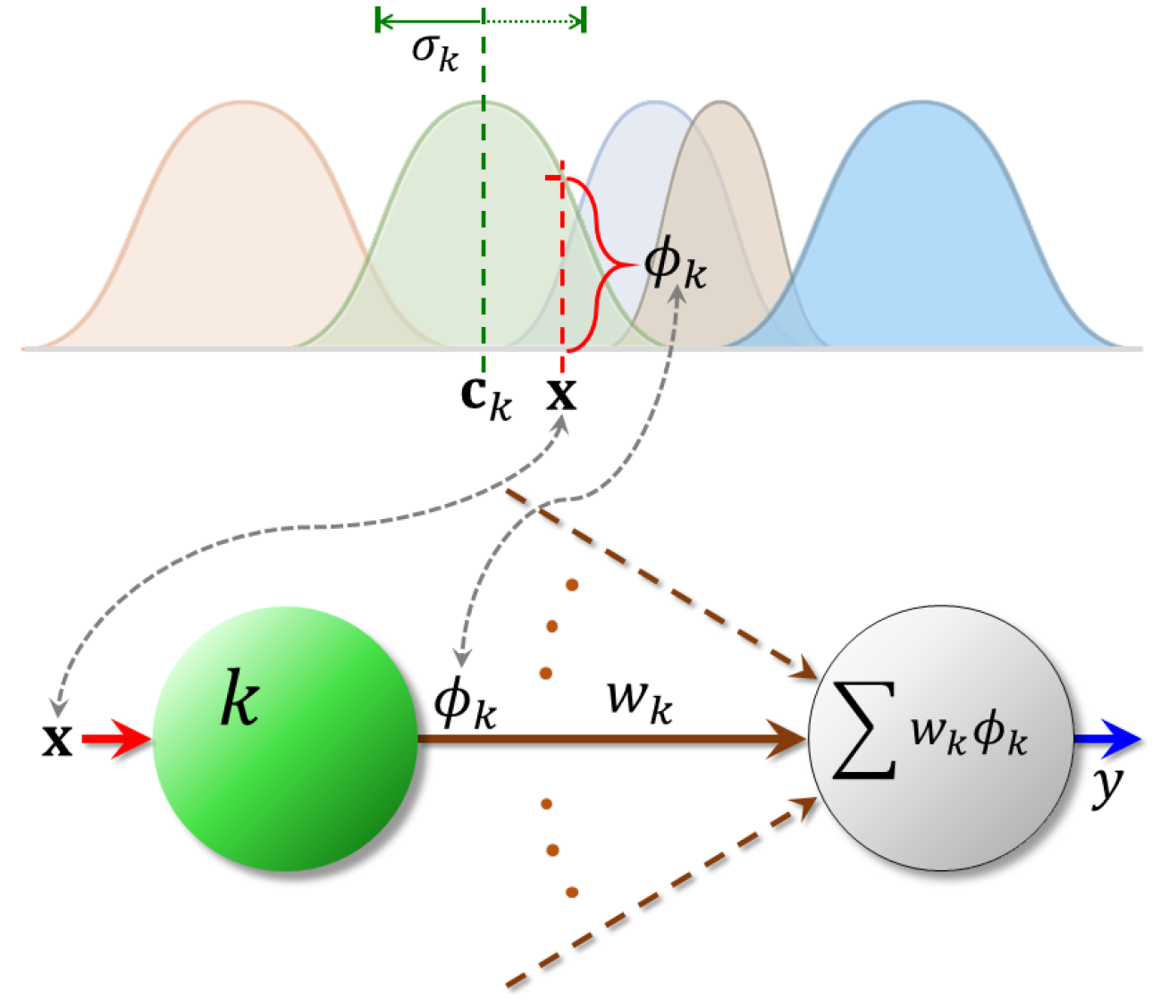
4.2. Radial Basis Function Networks

The radial basis function network (RBFN) [54,55] is another popular computational intelligence regression model that is topologically identical to an $M\times K\times 1$ neural network. In other words, an RBFN has M input neurons, a single hidden layer of K neurons, and only one output neuron. The sole purpose of the input layer, which contains M linear neurons, is to pass on M dimensional inputs to the hidden layer. The K neurons in the hidden layer are incorporated with nonlinear activation functions. The output neuron computes the weighted summation of the outputs from the hidden layer. Due to its strong resemblance to a shallow neural network, the RBFN is sometimes treated as a specific kind of NN. RBFNs have been successfully used in agricultural applications [56,57,58].

Unlike in NNs, the hidden neurons of the RBFN are designed to produce localized responses. The activation function of any hidden neuron has an M dimensional parameter called its center. The closer an input is to its center, the higher the neuron’s output. In this manner, the network’s hidden neurons simulate sensory cells of the peripheral nervous system, which have localized receptive fields.

Suppose $\mathbf{x}$ ($\mathbf{x}\in {\mathbb{R}}^M$) is the network’s input. Each hidden neuron k (where $k\in \{1\cdots K\}$) receives $\mathbf{x}$ from the input layer, and produces an output $f\left(\right||\mathbf{x}-{\mathbf{c}}_k|\left|\right)$, where $\left|\right|·\left|\right|$ denotes a vector norm operator (e.g., length). Gaussian nonlinearities are the most widely used activation functions. In this case, the output of the k^th hidden neuron, denoted as ${\varphi }_k$, is obtained according to the following expression,

$${\varphi }_k=e^{\frac{1}{{\sigma }_k}{\left|\right|\mathbf{x}-{\mathbf{c}}_k\left|\right|}^2}$$

(12)

The quantity ${\sigma }_k$ in (12) is an optional width parameter of the k^th hidden neuron. When dealing with training samples that are distributed evenly within the input space, all hidden neurons may be assigned the same widths $\sigma$.

With $w_k$ ($k\in 1\cdots K$) being network weights, the RBFN’s output y is the weighted sum ${\sum }_k{w}_k{\varphi }_k$. Using (12), y can be expressed directly in terms of the input $\mathbf{x}$ as,

$$y=\sum _k{w}_k{e}^{\frac{1}{{\sigma }_k}{\left|\right|\mathbf{x}-{\mathbf{c}}_k\left|\right|}^2}$$

(13)

Figure 7 depicts the main quantities of an RBFN.

The RBFN’s parameters in $\Theta$ are all its weights $w_k$ and centers ${\mathbf{c}}_k$. If necessary to train the network’s widths ${\sigma }_k$, they are also included in $\Theta$. Due to the use of localized activation functions, the number of hidden neurons K required by the RBFN increases exponentially with the input dimensionality M. Hence the effectiveness of RBFNs is limited to tasks involving low dimensional data (up to $M=$ 6 or 7). Even in such tasks, RBFNs require significantly more hidden neurons than NNs. As the trade-off for this limitation, RBFNs offer faster training, often by a few orders of magnitude. This speedup over Equation (6) is achieved when the centers, widths, and weights are trained separately [59].

A popular method to train the centers of the hidden neurons is by using K-means clustering [60]. For each hidden neuron k, a subset ${\mathcal{N}}_k$ of samples in training set ${\mathcal{S}}_t$ is obtained. This subset consists of all samples that are closer to the neuron’s center ${\mathbf{c}}_k$ than to ${\mathbf{c}}_{k^{\prime }}$ of any other neuron $k^{\prime }$, $k^{\prime }\ne k$. The center of each hidden neuron is made equal to the average of all samples $\mathbf{x}\left(n\right)$ in ${\mathcal{N}}_k$. The two steps can be expressed, as shown below,

$$\begin{array}{cc}\hfill & {\mathbf{c}}_k\leftarrow \frac{1}{|{\mathcal{N}}_k|}\sum _{n\in {\mathcal{N}}_k}\mathbf{x}\left(n\right),\mathrm{where},\hfill \\ \hfill & {\mathcal{N}}_k=\{n\in {\mathcal{S}}_t|k^{\prime }\ne k,\left|\right|\mathbf{x}\left(n\right)-{\mathbf{c}}_k\left|\right|<\left|\right|\mathbf{x}\left(n\right)-{\mathbf{c}}_{k^{\prime }}\left|\right|\}\hfill \end{array}$$

(14)

A relatively small number of iterations of (14) is enough to train the centers of all hidden neurons. Their widths can be fixed at some constant value such that ${\sigma }_k=\sigma$, $k\in \{1\cdots K\}$. Alternately, the nearest neighbor heuristic can be applied to determine each ${\sigma }_k$ separately, such as,

$${\sigma }_k=c\underset{k^{\prime }\ne k}{\mathrm{argmin}}\left|\right|{\mathbf{c}}_k-{\mathbf{c}}_{k^{\prime }}\left|\right|$$

(15)

The quantity c in (15) is an algorithmic constant.

For the ${\mathcal{L}}_1$ or the Hüber loss functions, the weight parameters ${\mathbf{w}}_k$ must be trained in an iterative manner using (6). When the ${\mathcal{L}}_2$ loss is used, the Moore-Penrose pseudoinverse formula provides a simpler method to obtain the weights. Let $\mathbf{w}\in {\mathbb{R}}^K$ be the vector of all weights. Similarly, let $\mathbf{\varphi }\left(n\right)\in {\mathbb{R}}^K$ ($n\in {\mathcal{S}}_t$) be the vector of outputs of the hidden neurons, determined using (12)) with input $\mathbf{x}\left(n\right)$. It can be observed that the RBFN’s output is $y\left(n\right)={\mathbf{\varphi }}^{\mathrm{T}}\left(n\right)\mathbf{w}$ (where ${·}^{\mathrm{T}}$ is the transpose operator).

To observe how the pseudoinverse formula works, let us construct an activation matrix $\Phi \in {\mathbb{R}}_{+}^{|{\mathcal{S}}_t|\times K}$, whose n^th row is ${\mathbf{\varphi }}^{\mathrm{T}}\left(n\right)$. Whence $\mathbf{y}=\Phi \mathbf{w}$ is the $|{\mathcal{S}}_t|\times 1$ vector of all outputs of the RBFN. If $\mathbf{t}\in {\mathbb{R}}^{|{\mathcal{S}}_t|}$ is the corresponding vector of all target values, the mean squared ${\mathcal{L}}_2$ loss is the expression ${\mathcal{L}}_2={\left|\right|\mathbf{y}-\mathbf{t}\left|\right|}^2$. The weight vector that minimizes this loss is $\underset{\mathbf{w}}{\mathrm{argmin}}{\left|\right|\Phi \mathbf{w}-\mathbf{t}\left|\right|}^2$.

If the number of training samples is more than the number of hidden neurons (i.e., $|{\mathcal{S}}_t|>K$), which is always the case in a real application, the matrix ${\Phi }^{\mathrm{T}}\Phi$ is non-singular. In this case, the expression for the loss minimizing weight vector $\mathbf{w}$ is determined as,

$$\mathbf{w}={\left({\Phi }^{\mathrm{T}}\Phi \right)}^{-1}{\Phi }^{\mathrm{T}}\mathbf{t}$$

(16)

The factor ${({\Phi }^{\mathrm{T}}\Phi )}^{-1}{\Phi }^{\mathrm{T}}$ in (16) is a matrix of size $K\times |{\mathcal{S}}_t|$. It is referred to as the pseudoinverse of $\Phi$ and denoted as ${\Phi }^{+}$.

In theory, all RBFN parameters can be trained iteratively using gradient descent. Although training the RBFN parameter vectors $\left[{\mu }_k\right]$ and $\left[{\sigma }_k\right]$ in this manner is fairly uncommon, and gradient descent is often used to train the weight vector $\mathbf{w}$. This is carried out as in Equation (6), with $\Theta$ replaced with $\mathbf{w}$. This method is applied to avoid numerical issues with matrix pseudoinversion and wherever the training algorithm is not based on the mean squared loss function.

Recent RBFN models use multivariate Gaussian distributions, where Equation (12) is replaced with,

$${\varphi }_k=e^{\frac{1}{2}{(\mathbf{x}-{\mathbf{c}}_k)}^{\mathrm{T}}{\Sigma }_k(\mathbf{x}-{\mathbf{c}}_k)}$$

(17)

In the above expression, the quantity ${\Sigma }_k\in {\mathbb{R}}^{M\times M}$ is a covariance matrix.

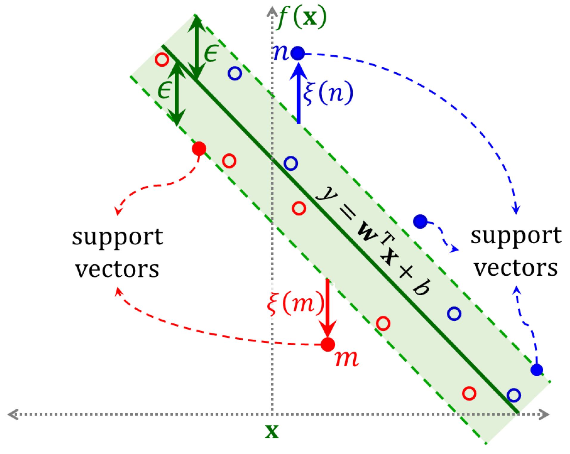
4.3. Support Vector Regression

SVRs are another class of CI models [61,62] that are widely used in various engineering and other applications [63]. SVRs have been used for regression applications in agriculture [64,65,66,67]. Unlike the other CI models discussed earlier, SVRs do not have any strong parallels in nature. Instead, they are specifically aimed at addressing the issue of model complexity, which is addressed below.

The simplest formulation is the linear SVR with $ϵ$-loss, as shown in Figure 8. Sample targets that lie within a margin of $\pm ϵ$ from the regression line do not incur any penalty, while those outside the margin incur penalties. Hence, the error arising from a sample pair $\left(\mathbf{x}\right(n),t(n\left)\right)$ is obtained as shown in (4). Denoting this error as $\xi \left(n\right)$, it can be readily established that the following constraints are satisfied,

$$\left\{\begin{array}{c}\xi \left(n\right)\ge 0\hfill \\ t\left(n\right)-{\mathbf{w}}^{\mathrm{T}}\mathbf{x}\left(n\right)-b\le ϵ+\xi \left(n\right)\hfill \\ {\mathbf{w}}^{\mathrm{T}}\mathbf{x}\left(n\right)+b-t\left(n\right)\le ϵ+\xi \left(n\right)\hfill \end{array}\right.$$

(18)

When the above conditions are satisfied, the loss is simply the sum of all errors, ${\sum }_n\xi \left(n\right)$.

It has been demonstrated that the gap between the validation and training losses (i.e., $\mathcal{L}\left({\mathcal{S}}_v\right)-\mathcal{L}\left({\mathcal{S}}_t\right)$) can be lowered by increasing $ϵ$, or alternately by decreasing ${\left|\right|\mathbf{w}\left|\right|}_2$ while $\pm ϵ$ is a constant [68]. This term can be recognized as the LASSO regularizer.

With C being an algorithmic constant, the optimal regression model can be obtained as the solution to the following constrained optimization problem,

$$\left\{\begin{array}{cccc}\hfill {\displaystyle \underset{\mathbf{w},b,\xi }{min}}& \multicolumn{3}{c}{\frac{1}{2}{\mathbf{w}}^{\mathrm{T}}\mathbf{w}+C\sum _{n\in {\mathcal{S}}_t}\xi \left(n\right)}\\ \mathrm{s}.\mathrm{t}.\hfill & \left(18\right)\hspace{1em}\mathrm{is}\mathrm{true}\hfill \end{array}\right.$$

(19)

The above problem (19) to obtain the SVR is in primal form. Classical optimization theory (cf. [69,70]) illustrates that for every primal problem, a dual problem can be constructed using the Lagrange multipliers of the primal constraints as its variables. The optimization theory establishes that under certain constraint qualifications, the optima of the primal and dual problems coincide at a saddle point. The dual form of (19) can be derived readily [68]. Ignoring the constraints $\xi \left(n\right)\ge 0$ and using the symbols ${\lambda }_{+}\in {\mathbb{R}}_{+}^{|{\mathcal{S}}_t|}$ and ${\lambda }_{-}\in {\mathbb{R}}_{+}^{|{\mathcal{S}}_t|}$ as the Lagrange multiplier vectors of the other constraints in (18), the dual problem can be formulated in the following manner,

$$\left\{\begin{array}{cccc}\hfill {\displaystyle \underset{{\lambda }_{+},{\lambda }_{-}}{min}}& \multicolumn{3}{c}{\frac{1}{2}{({\lambda }_{+}-{\lambda }_{-})}^{\mathrm{T}}\mathbf{K}({\lambda }_{+}-{\lambda }_{-})+{\lambda }_{+}^{\mathrm{T}}(ϵ\mathbf{1}-\mathbf{t})+{\lambda }_{-}^{\mathrm{T}}(ϵ\mathbf{1}+\mathbf{t})}\\ \hfill \mathrm{s}.\mathrm{t}.& {\mathbf{1}}^{\mathbf{T}}({\lambda }_{+}-{\lambda }_{-})=0\hfill \\ \hfill & \mathbf{0}\le {\lambda }_{+},{\lambda }_{+}\le C\mathbf{1}\hfill \end{array}\right.$$

(20)

The element in the m^th row and n^th column of the symmetric matrix $\mathbf{K}\in {\mathbb{R}}_{+}^{|{\mathcal{S}}_t|}$ in (20) is $\mathbf{x}{\left(m\right)}^{\mathrm{T}}\mathbf{x}\left(n\right)$. The bias b and the normal vector $\mathbf{w}$ can be obtained from the dual solution, although $\mathbf{w}$ is not required.

In more generalized settings, input samples can lie in any arbitrary Hilbert space. The inner product of the m^th and n^th samples is represented as $\langle \mathbf{x}\left(m\right),\mathbf{x}\left(n\right)\rangle$. The matrix $\mathbf{K}$ will contain pairwise inner products of such samples.

Nonlinear SVRs implicitly apply a transformation $\varphi (·)$ from the input space $\mathcal{S}$ to an unknown Hilbert space [61]. Under these circumstances, the $(m,n)$^th element of $\mathbf{K}$, which we now denote as $K\left(\mathbf{x}\right(m),\mathbf{x}(n\left)\right)$, is obtained as provided below,

$$K\left(\mathbf{x}\right(m),\mathbf{x}(n\left)\right)=\langle \varphi \left(\mathbf{x}\right(m\left)\right),\varphi \left(\mathbf{x}\right(n\left)\right)\rangle$$

(21)

The function $K:\mathcal{S}\times \mathcal{S}\to {\mathbb{R}}_{+}$ is referred to as the kernel function. Mercer’s theorem states that as long as the kernel satisfies a few conditions, there must exist some transformation $\varphi :\mathcal{S}\to \mathbb{H}$ satisfying (21). As long as these conditions are met, the matrix $\mathbf{K}$ obtained from every possible sample set will be symmetric and positive definite. In other words, kernel functions can be devised without even considering the mapping $\varphi (·)$; this mapping, along with its range in Hilbert space $\mathbb{H}$ can remain unknown. This is a remarkable feature of SVR models. In engineering applications, any symmetric, non-negative measure of similarity between pairs of samples can be adopted as the kernel function. For instance, Gaussian kernels $e^{\frac{1}{\sigma }{\left|\right|\mathbf{x}\left(m\right)-\mathbf{x}\left(n\right)\left|\right|}^2}$, or ${\mathcal{L}}_p$-normed kernels $\left|\right|\mathbf{x}\left(m\right)-{\mathbf{x}\left(n\right)\left|\right|}_p$ can be adopted for inputs that lie in a Euclidean space ${\mathbb{R}}^M$. In bio-informatics, where samples may consist of DNA strands that are sequences of the letters C, T, G, and A, the kernel may vary negatively with the minimum edit distance between every pair of samples.

For each sample, $\mathbf{x}\left(n\right)$ that is strictly within the $\pm ϵ$ margin of the regression line (see Figure 8), the corresponding dual variables ${\lambda }_{\pm }\left(n\right)$ obtained from (20) will be zeros. It is only when the sample lies either on the margin’s boundaries or outside it that yields either ${\lambda }_{+}\left(n\right)>0$ or ${\lambda }_{-}\left(n\right)>0$. These samples are the support vectors. The set of all support vectors is,

$$\mathcal{V}=\left\{n\right|{\lambda }_{+}\left(n\right)>0\mathrm{or}{\lambda }_{-}\left(n\right)>0\}.$$

(22)

Given an unknown sample $\mathbf{x}$, the estimated output y can be obtained using the kernels of $\mathbf{x}$ and the support vectors in $\mathcal{V}$,

$$y=\sum _{n\in \mathcal{V}}({\lambda }_{+}\left(n\right)-{\lambda }_{-}\left(n\right))K(\mathbf{x}\left(n\right),\mathbf{x})+b.$$

Although not provided in this article, the bias b can be obtained readily from the dual form in (20).

As long as the training set ${\mathcal{S}}_t$ is small enough so that it is computationally feasible to compute the matrix $\mathbf{K}$ and store in memory, quadratic programming can be applied directly to solve (20). Otherwise, there are a plethora of iterative training algorithms [71,72,73], that are well-equipped to train SVRs with larger data sets. SVRs can be formulated using other losses and regularizers as well.

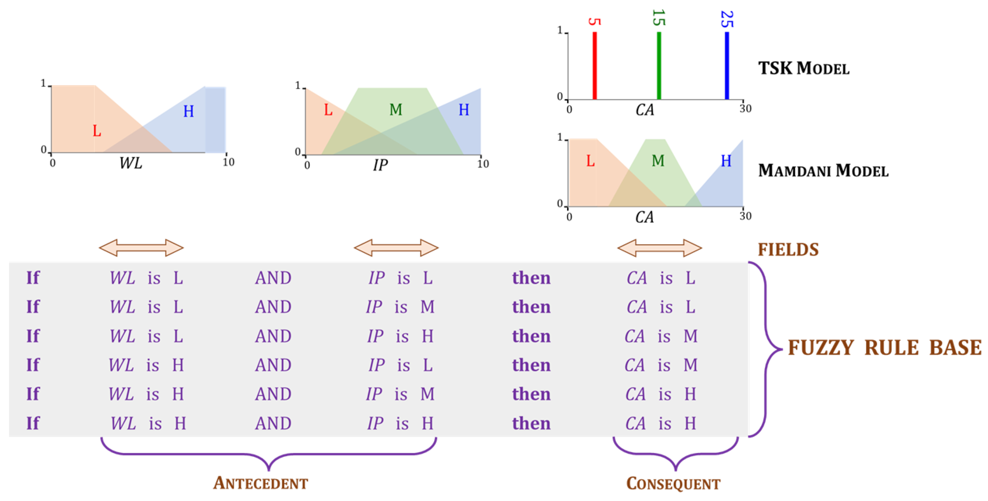
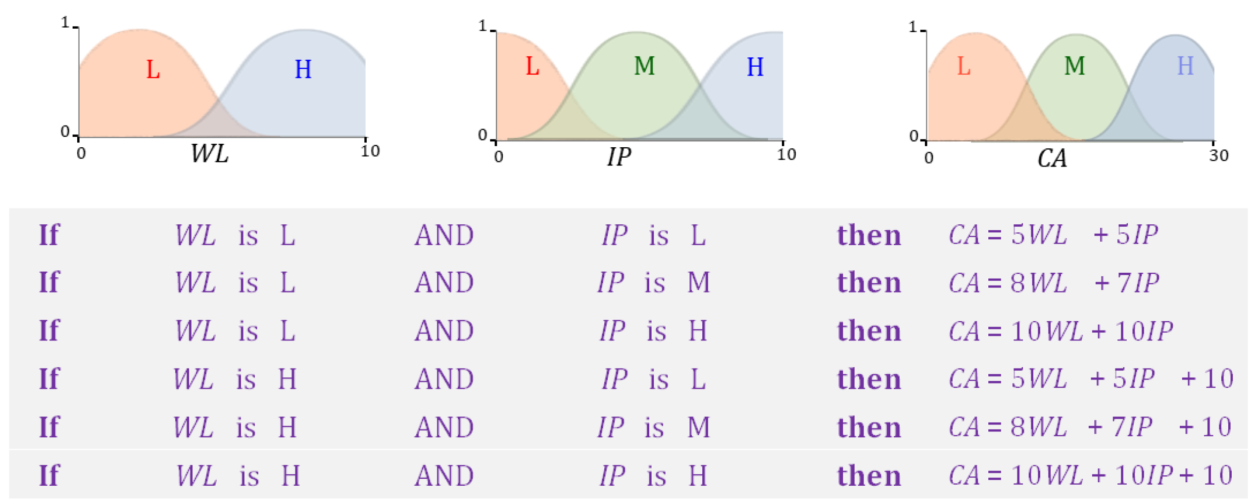
4.4. Fuzzy Inference Systems

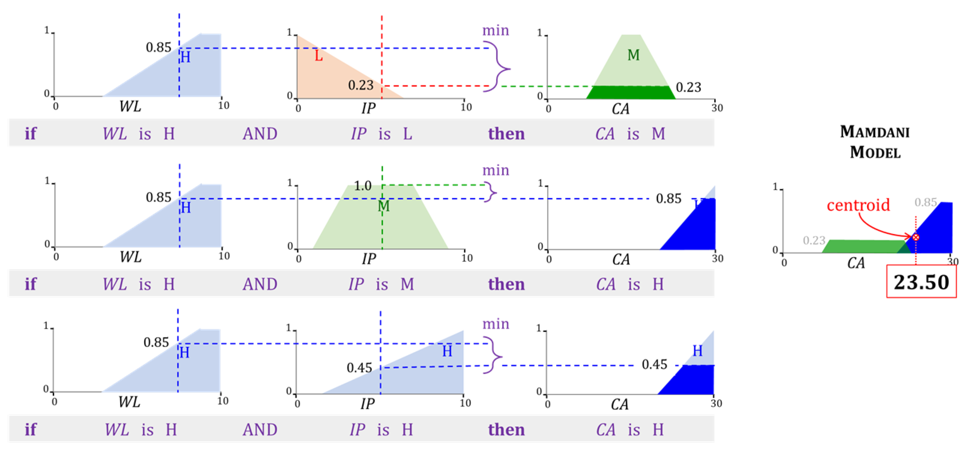
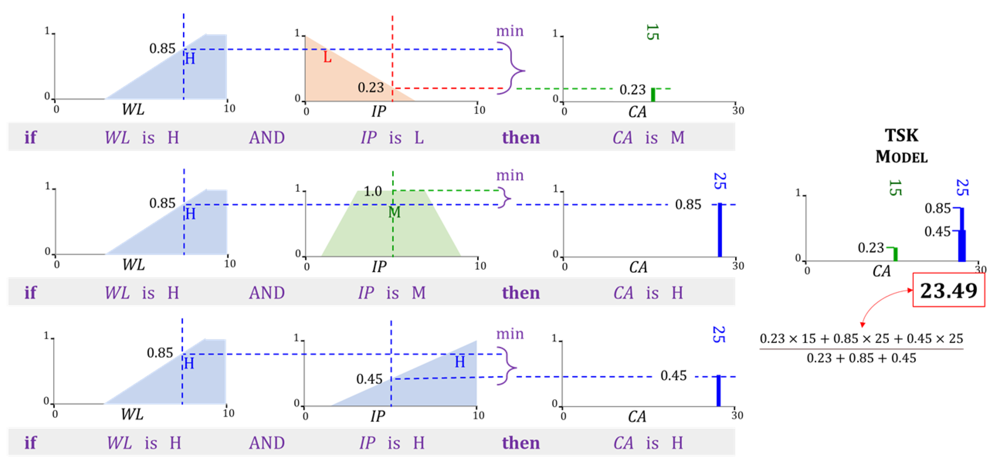
FIS is a CI model that is inspired by decision-making processes in humans. It uses fuzzy sets to capture the inherent vagueness in human verbal reasoning. The fuzzy set theory extends the classical concept of a set (called a ‘crisp’ set in fuzzy terminology) by incorporating such imprecision. The manner in which it does so is described next.

Any element x from the universe of discourse $\mathbb{U}$ can either be in a given crisp set A, where $A\subset \mathbb{U}$ (i.e., $x\in A$) or not in it (i.e., $x\notin A$). Accordingly, a binary membership function ${\mu }_A:\mathbb{U}\to \{0,1\}$ can be defined such that ${\mu }_A\left(x\right)=1$ iff $x\notin A$, otherwise ${\mu }_A\left(x\right)=0$ iff $x\notin A$. The membership function of a fuzzy set A is allowed to have any real value within the interval $[0,1]$, i.e., ${\mu }_A:\mathbb{U}\to [0,1]$. The numerical value of ${\mu }_A\left(x\right)$ indicates the degree to which x is included in A. For example, let T be the set of tall students in a class. If T is a crisp set, there must be a minimum cutoff for tallness. Let this cutoff be 5′10″. Hence, Jack and Jill, whose heights are 5′9″ and 6′1″, have memberships ${\mu }_T\left(\mathrm{Jack}\right)=0$, and ${\mu }_T\left(\mathrm{Jill}\right)=1$ in. On the other hand, if T is a fuzzy set, then memberships such as ${\mu }_T\left(\mathrm{Jack}\right)=0.7$, and ${\mu }_T\left(\mathrm{Jill}\right)=0.99$ are possible, indicating that Jack is very close to being tall, whereas Jill is definitely tall.

When the universe of the discourse is a continuous variable, memberships can be defined in terms of functions of real arguments $\mu :\mathbb{R}\to [0,1]$. The Gaussian, trapezoidal, and triangular functions are commonly used for memberships. The Gaussian membership of a scalar input x to the fuzzy set $A\subset \mathbb{U}$ is $e^{-(x-\mu )/\sigma }$. The trapezoidal membership can be defined using four parameters, a, b, c, and d ($a\le b<c\le d$),

$${\mu }_A\left(x\right)=\left\{\begin{array}{cc}0,\hfill & \mathrm{if}x<a;\hfill \\ \frac{x-a}{b-a},\hfill & \mathrm{if}a\le x<b;\hfill \\ 1,\hfill & \mathrm{if}b\le x<c;\hfill \\ \frac{d-x}{d-c},\hfill & \mathrm{if}c\le x<d;\hfill \\ 0,\hfill & \mathrm{if}d\le x.\hfill \end{array}\right.$$

(23)

The triangle membership function requires only three parameters, a, b, and c ($a\le b\le c$),

$${\mu }_A\left(x\right)=\left\{\begin{array}{cc}0,\hfill & \mathrm{if}x<a;\hfill \\ \frac{x-a}{b-a},\hfill & \mathrm{if}a\le x<b;\hfill \\ \frac{c-x}{c-b},\hfill & \mathrm{if}b\le x<c;\hfill \\ 0,\hfill & \mathrm{if}c\le x.\hfill \end{array}\right.$$

(24)

Gaussian memberships, as well as those in (23) and (24), have peak values of unity. Although this is common practice in real-world applications, fuzzy sets can also admit any other membership function as long as its maximum lies anywhere in $(0,1]$. The complement $\overline{A}$ of the fuzzy set A can be readily defined in terms of the membership function as ${\mu }_{\overline{A}}=1-{\mu }_A$. A fuzzy singleton—say B, is a fuzzy set that is fully parametrized by a constant $v_B$, where $v_B\in \mathbb{R}$, such that for the input $y\in \mathbb{R}$,

$${\mu }_B\left(y\right)=\left\{\begin{array}{cc}1,\hfill & \mathrm{if}y=v_B;\hfill \\ 0,\hfill & \mathrm{otherwise}.\hfill \end{array}\right.$$

(25)

The operations of union (∪) and intersection (∩) in crisp sets correspond to conjunction (AND) and disjunction (OR) in Boolean algebra. In terms of membership functions, the union $A\cup B$ and intersection $A\cap B$ of the sets A and B are ${\mu }_{A\cup B}={\mu }_A\mathrm{OR}{\mu }_A$, and ${\mu }_{A\cap B}={\mu }_A\mathrm{AND}{\mu }_A$. Union and intersection of fuzzy sets can be realized in various ways [74], using t-conorms and t-norms. A popular choice is to use $\max (\cdots )$ as the t-conorm operator and $\min (\cdots )$ as the t-norm. In this case, ${\mu }_{A\cup B}=\max \{{\mu }_A,{\mu }_B\}$ and ${\mu }_{A\cap B}=\min \{{\mu }_A,{\mu }_B\}$. In our previous example, suppose S is the fuzzy set of smart students and ${\mu }_S\left(\mathrm{Jill}\right)=0.75$, then ${\mu }_{S\cup T}\left(\mathrm{Jill}\right)=\max \{0.75,0.99\}=0.99$ and ${\mu }_{S\cap T}\left(\mathrm{Jill}\right)=\min \{0.75,0.99\}=0.75$.

A FIS encapsulates human knowledge through a fuzzy rule base. Each rule in the base consists of two parts, an antecedent and a consequent, and is written in the format, “$\mathbf{If}$ Antecedent $\mathbf{then}$ Consequent”. If the input to the model is an M-dimensional vector $\mathbf{x}$ and its output is an M-dimensional vector $\mathbf{y}$, the antecedents and consequents are made up of M and N fields. The generic format of a rule with index $k\in 1,2,\cdots ,K$ is as shown below,

$$\mathbf{If}\underset{\mathrm{A}\mathrm{NTECEDENT}}{\underbrace{x_1\mathrm{is}{A}_1^k\diamond x_2\mathrm{is}{A}_2^k\cdots \diamond x_M\mathrm{is}{A}_M^k}}\mathbf{then}\underset{\mathrm{C}\mathrm{ONSEQUENT}}{\underbrace{y_1\mathrm{is}{B}_1^k\cdots \diamond y_N\mathrm{is}{B}_N^k}}.$$

(26)

Each diamond symbol (⋄) in (26) represents an AND or an OR operator.

The order in which these operations are applied may either be in accordance with an established convention or, alternately, specified explicitly by inserting brackets at appropriate places. Mathematically speaking, the j^th field in the antecedent of the fuzzy rule in Equation (26), “$x_j\mathrm{is}{A}_j$” is the membership, ${\mu }_{A_j}\left(x_j\right)$. In a similar fashion, the i^th field in the consequent is ${\mu }_{B_i}\left(y_i\right)$. Figure 9 shows a simple rule base with $K=6$ rules.

There are two kinds of FIS, differing only in the way the sets $B_i$ in the consequent’s i^th field ($i\in \{1,2,\cdots ,N\}$) are defined. In the Mamdani model [75], they are allowed to be fuzzy sets. As a result of this flexibility, a Mamdani FIS can easily apply verbal descriptions of the consequents. On the other hand, in the Takagi-Sugeno-Kang (TSK) model [76,77], each $B_i$ must be a singleton, as in Equation (25). A TSK model renders the FIS more amenable to mathematical treatment. Figure 9 shows examples of the Mamdani and TSK models.

The various steps involved in mapping an input to its output will be illustrated using the examples shown in Figure 10 (Mamdani model) and Figure 11 (TSK model). The steps are briefly described below.

(i)

Fuzzification: This step is carried out separately in each antecedent field “$x_j\mathrm{is}{A}_j^k$” and for each rule k. It involves computing the values of the memberships ${\mu }_{A_j^k}\left(x_j\right)$ using the numerical values of the input element $x_j$.

(ii)

Aggregation: In this step, AND and OR operations are applied as appropriate to each rule in the FIS. The rules in the FIS shown in Figure 10 and Figure 11 only involve conjunctions (AND) that are implemented through the $\min (·)$ t-norm. The aggregated membership is referred to as its rule strength. The strength of rule k is,

$${\mu }_A^k=\bigcup _j{\mu }_{A_j^k}\left(x_j\right).$$

(27)

(iii)

Inference: The strength of each rule is applied to its consequent. Each rule k in our example contains only one consequent field. Its membership function ${\mu }_{B^k}$ is limited to a maximum of ${\mu }_{A^k}$. For every rule, k in k, a two-dimensional region ${\mathcal{R}}^k$ is identified in the Mamdani model. Since the TSK model involves only singletons at this step, only a two-dimensional point ${\mathcal{R}}^k$ is necessary. Accordingly,

$${\mathcal{R}}^k=\left\{\begin{array}{cc}\left\{(y^k,z^k)\right|y^k\in [0,y_{max}],z^k\in [0,\max ({\mu }_{B^k}\left(y\right),{\mu }_{A^k})]\},\hfill & \mathrm{Mamdani};\hfill \\ (v_{B^k},{\mu }_{A^k}),\hfill & \mathrm{TSK}.\hfill \end{array}\right.$$

(28)

In the example shown in Figure 10, the upper limit $y_{max}=30$.

(iv)

Defuzzification: The value of the FIS’s output is determined in the last step. The Mamdani FIS in Figure 10 uses the centroid defuzzification method. The regions ${\mathcal{R}}^k$ are unified into a single region $\mathcal{R}$. The final output is the x-coordinate of the centroid of $\mathcal{R}$. The TSK model in Figure 11 uses a weighted sum to obtain the output y of the FIS. Mathematically,

$$y=\left\{\begin{array}{cc}{\left[{\int }_{\mathcal{R}}d\mathcal{R}\right]}^{-1}{\int }_{\mathcal{R}}{z}^{k}d\mathcal{R},\hfill & \mathrm{Mamdani};\hfill \\ {\left[\sum _k{\mu }_{A^k}\right]}^{-1}\sum _k{v}_{B^k}{\mu }_{A^k},\hfill & \mathrm{TSK}.\hfill \end{array}\right.$$

(29)

In the above expression, $\mathcal{R}={\displaystyle \bigcup _k}\mathcal{R}$. It is evident from the above description, that the inference and defuzzification step in a Mamdani FIS is more computationally intensive in comparison to that in the TSK model. There are several other methods to obtain the output of a FIS. For details, the interested reader is referred to [78,79]. The Mamdani model [80,81,82] as well as the TSK model [83,84,85,86,87] have been used frequently in agricultural research.

Figure 10. Mamdani FIS. The inputs to the FIS in Figure 9 are $WL=7.5$ and $WL=5.0$ (dotted vertical lines), and the output is $y=23.50$). The first three rules in Figure 9 with $WL=\mathrm{H}$ are ignored since ${\mu }_{\mathrm{L}\left(7.5\right)=0)}$. The dark-shaded regions are ${\mathcal{R}}^k$ of the relevant rules.

Figure 10. Mamdani FIS. The inputs to the FIS in Figure 9 are $WL=7.5$ and $WL=5.0$ (dotted vertical lines), and the output is $y=23.50$). The first three rules in Figure 9 with $WL=\mathrm{H}$ are ignored since ${\mu }_{\mathrm{L}\left(7.5\right)=0)}$. The dark-shaded regions are ${\mathcal{R}}^k$ of the relevant rules.

Figure 11. TSK FIS. The inputs to the FIS in Figure 9 are $WL=7.5$ and $WL=5.0$ (dotted vertical lines), and the output is $y=23.49$. The first three rules in Figure 9 with $WL=\mathrm{H}$ are ignored since ${\mu }_{\mathrm{L}}\left(7.5\right)=0)$. In the other rules, the values of $v_{B^k}$ are 15, 25, and 25.

Figure 11. TSK FIS. The inputs to the FIS in Figure 9 are $WL=7.5$ and $WL=5.0$ (dotted vertical lines), and the output is $y=23.49$. The first three rules in Figure 9 with $WL=\mathrm{H}$ are ignored since ${\mu }_{\mathrm{L}}\left(7.5\right)=0)$. In the other rules, the values of $v_{B^k}$ are 15, 25, and 25.

4.5. Adaptive Neuro-Fuzzy Inference Systems

A TSK model with fuzzy rules as in (26) is often referred to as a zero-order FIS. An ANFIS is based on a zero or higher order TSK model, that is arranged in a manner resembling an NN [88,89,90]. ANFIS models frequently use first-order TSK rule bases. Assuming a scalar output y, the format of the k^th rule in such a first-order TSK model is,

$$\mathbf{If}{x}_1\mathrm{is}{A}_1^k\diamond \cdots \diamond x_M\mathrm{is}{A}_M^k\mathbf{then}y=b_0^k+b_1^k{x}_1+\cdots +b_M^k{x}_M.$$

(30)

The consequent in Equation (30) is a linear expression for y in terms of $\mathbf{x}$, with $M\times K$ coefficients, $b_j^k$ (where $j\in 1,\cdots ,M$ and $k\in 1,\cdots ,K$). To simplify its training, the membership functions in the ANFIS rules’ antecedents are usually restricted to Gaussian [90]. Figure 12 shows an example of a first-order TSK model.

Figure 13 illustrates the ANFIS corresponding to the first-order TSK rule set shown in Figure 12. The parameters of the membership functions of each input variable are trainable quantities. For Gaussian memberships, they are ${\sigma }_j^k,{\mu }_j^k$, where $j\in \{1,\cdots ,M\}$, and k is the index of a rule). The coefficients in the consequent side of each such rule, which are $b_j^k$, $j\in \{0,1,\cdots ,M\}$ are also trainable. All trainable quantities constitute the parameter vector $\Theta$ of the ANFIS.

There are five layers in the ANFIS model, which are as follows.

(i)

Fuzzifying layer: The role of the first layer is to fuzzify scalar elements $x_j,j\in \{1\cdots M\}$ of the input $\mathbf{x}$. It involves computing the memberships ${\mu }_{A_j^k}\left(x_j\right)$ in (31).

(ii)

Aggregating layer: This layer performs aggregation. When all ⋄ operators in (30) are conjunctions, the output of the k^th unit in the second layer is obtained using the expression,

$${\mu }_A^k=\prod _j{\mu }_{A_j^k}\left(x_j\right).$$

(31)

(iii)

Normalizing layer: This is the third layer of the ANFIS, whose role is to normalize the incoming aggregated memberships, ${\mu }_A^k$ from the previous layer. The output of its k^th unit is,

$${\widehat{\mu }}_A^k=\frac{{\mu }_A^k}{{\sum }_{k^{\prime }}{\mu }_A^{k^{\prime }}}.$$

(32)

(iv)

Consequent layer: The output of the k^th unit of the fourth layer is,

$$y^k={\widehat{\mu }}_A^k\left(b_0^k+\sum _j{b}_j^k{x}_j\right).$$

(33)

(v)

Output layer: The final layer of the ANFIS performs a summation of the consequent outputs $y^k$,

$$y=\sum _k{y}^k.$$

(34)

The quantity y is the output of the ANFIS.

Several methods have been proposed to train the parameters of an ANFIS model [91]. Much research has been directed towards gradient descent approaches ((6)) resembling BP [89,92]. Such approaches have been used in agriculture [93,94,95]. A Levenberg-Marquardt approach has been suggested recently [96]. Stochastic metaheuristics such as GAs [97] and PSO [98] have also been investigated. Hybrid approaches combining them are widely used to train ANFISs [99]. A comparison of three metaheuristics has been reported in [100] for an agriculture-related application.

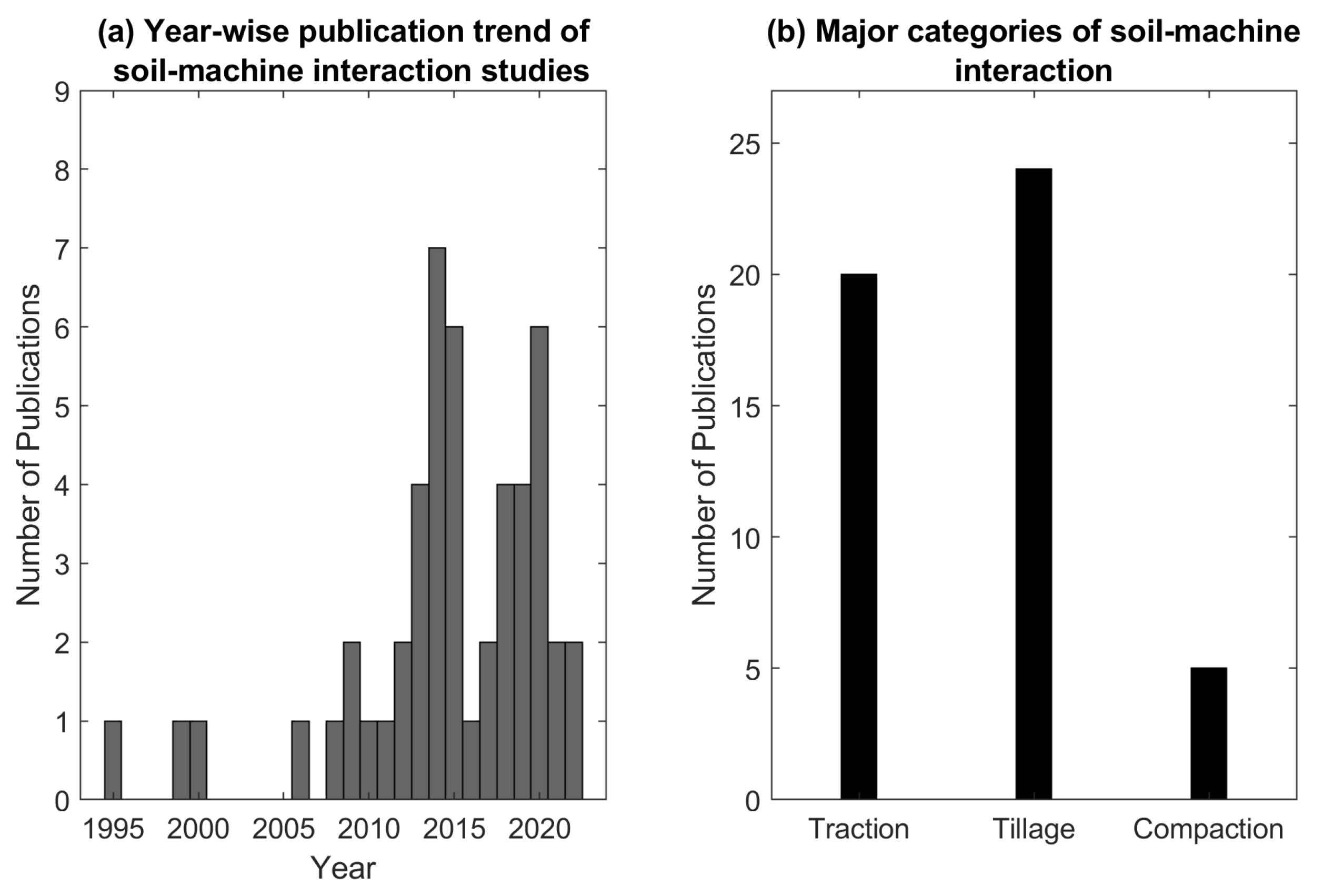
5. Soil–Machine Interaction Studies: A Brief Survey

5.1. Literature Survey Methodology

In recent decades, CI methods have been extensively studied in agriculture, particularly in crop management, insect–pest management, irrigation scheduling, precision agriculture, input application optimization, yield prediction, and so on [80]. Initially, we collected research articles for the period ranging from 1990 to 2022, from multiple online databases such as Web of Science, Scopus, Science Direct, Google Scholar, Wiley, and Springer Link. More than 150 research articles were collected in the preliminary screening stage. Out of the 150 articles, only 50 articles directly related to the CI application on traction, tillage, and compaction were selected. Figure 14 shows the year-wise and categorical distribution of the selected articles where CI methods were employed.

5.2. Traction

In traction studies, an individual traction element (wheel, track) or entire off-road vehicle is tested in a controlled laboratory setup or prepared or un-prepared fields for its performance optimization. The major performance parameters are drawbar pull, traction efficiency, slip, and fuel consumption, which are optimized as a function of numerous variables pertaining to the machine, operational setup, and soil properties. A summary of CI models developed in selected traction studies is shown in Table 1.

An off-road vehicle (tractor or skidder) used in agriculture and forestry is specially designed for drawbar work, i.e., pulling or pushing the implements. Drawbar power is a product of drawbar pull and vehicle velocity in the travel direction. The vehicle tire size and its inflation pressure increase the soil contact area, which improves the drawbar performance. The drawbar performance of the forestry skidder was studied [101] in soft soil to develop a multiple linear regression (MLR) and fully connected NN to predict the drawbar pull. For tractor energy management and optimization, the NN hybridized with GA, and the ANFIS was implemented to predict the drawbar pull energy [50], and net traction power [102]. The tractor’s drawbar pull varies with vehicle configuration, weight, and operating mode (2WD and 4WD). Thus, a FIS was proposed to estimate a drawbar pull [103]. In addition to tire size, the drawbar pull is also influenced by the tire geometrical parameters, which can be defined with 3D footprints. Thus, NN was implemented to understand the complex relationship between 3D tire footprints and generated the drawbar pull [104].

The traction device develops a force, parallel to the travel direction and transfers to the vehicle. The traction efficiency is a ratio of output power to input power to the device [105]. It is one of the most critical factors in traction studies and relates to energy saving. Several studies were conducted in a laboratory setup with a single-wheel tester to study the influence of the traction device’s operational parameters and soil properties on traction efficiency. Table 1 contains the various CI methods proposed to model the traction efficiency [106,107,108,109,110,111,112].

Motion resistance is an opposing force, that works against the traction device’s forward motion and accounts for all energy loss unrelated to slip [105]. Motion resistance is the difference between gross traction and net traction. A series of experiments were conducted on a driven wheel in a soil bin (clay loam) [113,114,115] that aimed to study the motion resistance influenced by various operating parameters, and predict motion resistance with the CI methods (NN & FIS).

The tractor is a major power source in agriculture. Therefore, it is essential to understand how tractor power can be best utilized for varying field conditions for efficient operation. The tractor loses the most power at the soil–tire interface, and its performance is influenced by operational and soil/terrain parameters. Therefore, the field performance of a 75 HP tractor was evaluated [116], and NN was proposed for predicting the tractor performance as a function of soil and tractor-implement variables. Likewise, NN and ANFIS were proposed to study the performance of tractor-implement operational parameters on traction efficiency [94] and wheel slip [117]. Specific fuel consumption is the most used and common indicator of tractor performance. Thus, NN was proposed to predict the fuel consumption of a 60 HP 2WD tractor [118].

Mobile robots and autonomous ground vehicles (AGV) are becoming popular on smart farms. Thus, the traction behavior of the ground vehicle was studied on a sloped soil bin, and NN predicted the traction, mobility, and energy requirement of the AGV [119].

Table 1. Traction studies which employed the CI methods.

Author & Year	Traction Device	Method	Input	Output
Hassan and Tohmaz (1995) [101]	Rubber-tire skidder	NN	Tire size, tire pressure, normal load, line of pull angle	Drawbar pull
Çarman and Taner (2012) [106]	Driven wheel	NN	Travel reduction	Traction efficiency
Taghavifar et al. (2013) [113]	Driven wheel	NN	Velocity, tire pressure, normal load	Rolling resistance
Taghavifar and Mardani (2013) [114]	Driven wheel	FIS	Velocity, tire pressure, normal load	Motion resistance coeff.
Taghavifar and Mardani (2014) [107]	Driven wheel	ANFIS	Velocity, wheel load, slip	Energy efficiency indices (Traction coeff. and traction efficiency)
Taghavifar and Mardani (2014) [108]	Driven wheel	NN	Velocity, wheel load, slip	Energy efficiency indices (Traction coeff. and traction efficiency)
Taghavifar and Mardani (2014) [109]	Driven wheel	NN	Soil texture, tire type, wheel load, speed, slip, inflation pressure	Traction force
Taghavifar and Mardani (2014) [115]	Driven wheel	NN & SVR	Wheel load, inflation pressure, velocity	Energy wasted
Taghavifar and Mardani (2015) [50]	Driven wheel	ANFIS	Wheel load, inflation pressure, velocity	Drawbar pull energy
Taghavifar et al. (2015) [102]	Driven wheel	NN-GA	Wheel load, inflation pressure, velocity	Available power
Ekinci et al. (2015) [110]	Single wheel tester	NN & SVR	Lug height, axle load, inflation pressure, drawbar pull	Traction efficiency
Almaliki et al. (2016) [116]	Tractor	NN	Moisture content, cone index, tillage depth, inflation pressure, engine speed, forward speed	Traction efficiency, drawbar pull, rolling resistance, fuel consumption
Pentos et al. (2017) [111]	Micro tractor	NN	Vertical load, horizontal deformation, soil Coeff., compaction, moisture content	Traction force and traction efficiency
Shafaei et al. (2018) [94]	Tractor	ANFIS, NN	Forward speed, plowing depth, tractor mode	Traction efficiency
Shafaei et al. (2019) [117]	Tractor	ANFIS, NN	Forward speed, plowing depth, tractor mode	Wheel slip
Shafaei et al. (2020) [103]	Tractor	FIS	Tractor weight, wheel slip, tractor driving mode	Drawbar pull
Pentos et al. (2020) [112]	Micro tractor	NN, ANFIS	Vertical load, horizontal deformation, soil Coeff., compaction, moisture content	Traction force and traction efficiency
Hanifi et al. (2021) [118]	Tractor (60 HP)	NN	Inflation pressure, axle load, drawbar force	Specific fuel consumption
Badgujar et al. (2022) [119]	AGV	NN	Slope, speed, drawbar	Traction efficiency, slip and power number
Cutini et al. (2022) [104]	Tractor	NN	Tire geometric parameters (area, length, width, depth), slip	Drawbar pull

Table 1. Traction studies which employed the CI methods.

Author & Year	Traction Device	Method	Input	Output
Hassan and Tohmaz (1995) [101]	Rubber-tire skidder	NN	Tire size, tire pressure, normal load, line of pull angle	Drawbar pull
Çarman and Taner (2012) [106]	Driven wheel	NN	Travel reduction	Traction efficiency
Taghavifar et al. (2013) [113]	Driven wheel	NN	Velocity, tire pressure, normal load	Rolling resistance
Taghavifar and Mardani (2013) [114]	Driven wheel	FIS	Velocity, tire pressure, normal load	Motion resistance coeff.
Taghavifar and Mardani (2014) [107]	Driven wheel	ANFIS	Velocity, wheel load, slip	Energy efficiency indices (Traction coeff. and traction efficiency)
Taghavifar and Mardani (2014) [108]	Driven wheel	NN	Velocity, wheel load, slip	Energy efficiency indices (Traction coeff. and traction efficiency)
Taghavifar and Mardani (2014) [109]	Driven wheel	NN	Soil texture, tire type, wheel load, speed, slip, inflation pressure	Traction force
Taghavifar and Mardani (2014) [115]	Driven wheel	NN & SVR	Wheel load, inflation pressure, velocity	Energy wasted
Taghavifar and Mardani (2015) [50]	Driven wheel	ANFIS	Wheel load, inflation pressure, velocity	Drawbar pull energy
Taghavifar et al. (2015) [102]	Driven wheel	NN-GA	Wheel load, inflation pressure, velocity	Available power
Ekinci et al. (2015) [110]	Single wheel tester	NN & SVR	Lug height, axle load, inflation pressure, drawbar pull	Traction efficiency
Almaliki et al. (2016) [116]	Tractor	NN	Moisture content, cone index, tillage depth, inflation pressure, engine speed, forward speed	Traction efficiency, drawbar pull, rolling resistance, fuel consumption
Pentos et al. (2017) [111]	Micro tractor	NN	Vertical load, horizontal deformation, soil Coeff., compaction, moisture content	Traction force and traction efficiency
Shafaei et al. (2018) [94]	Tractor	ANFIS, NN	Forward speed, plowing depth, tractor mode	Traction efficiency
Shafaei et al. (2019) [117]	Tractor	ANFIS, NN	Forward speed, plowing depth, tractor mode	Wheel slip
Shafaei et al. (2020) [103]	Tractor	FIS	Tractor weight, wheel slip, tractor driving mode	Drawbar pull
Pentos et al. (2020) [112]	Micro tractor	NN, ANFIS	Vertical load, horizontal deformation, soil Coeff., compaction, moisture content	Traction force and traction efficiency
Hanifi et al. (2021) [118]	Tractor (60 HP)	NN	Inflation pressure, axle load, drawbar force	Specific fuel consumption
Badgujar et al. (2022) [119]	AGV	NN	Slope, speed, drawbar	Traction efficiency, slip and power number
Cutini et al. (2022) [104]	Tractor	NN	Tire geometric parameters (area, length, width, depth), slip	Drawbar pull

5.3. Tillage

Tillage is classified into two major categories: (1) primary and (2) secondary tillage, based on purpose, tillage depth, and energy requirement. Primary tillage is an initial major soil working operation, aiming to open up any cultivable land, reduce soil strength, cover plants/residues, and rearrange soil aggregates [2]. It manipulates soil at a greater depth (15 to 30 cm), and moldboard, disk, chisel plow, and subsoiler are commonly used primary tillage tools.

Moldboard (MB) plow shatters soil, inverts furrow slices, and covers crop residues or grasses. As the plow bottom advances, it cuts, fails the ground, and forms furrow slices, which shows a periodic variation in the draft force. Therefore, a time-lagged recurrent neural network (RNN) was proposed to predict the dynamic draft as a function of one step ahead prediction [120] for various shaped tillage tools (MB, Korean, model plow). The MB plow consumes the highest energy compared to other tillage tools for a given depth [121,122]. Therefore, the researchers studied the performance of various types of MB plow in varying soil conditions for energy optimization. The developed CI methods are listed in Table 2 and explained briefly as follows: The ANFIS models were proposed for predicting the draft and specific draft of three-bottom MB plow [123]. The NN predicted the specific draft and fuel consumption of a tractor-mounted MB plow under varying operating conditions [124]. Similarly, the NN was proposed for general-purpose MB plow’s draft, and energy requirement [122].

The MB plow has a sliding plow bottom that slides through the soil. The sliding friction is one of the primary reasons for the MB plow’s higher draft and energy requirement. On the contrary, a disk plow is equipped with concave rolling disks, i.e., a rolling plow bottom designed to reduce friction through rolling action. The energy requirement of the disk plow is significantly lower than the MB plow. Thus, the NN was proposed to predict the disk plow draft and energy requirement [125,126].

Deep tillage (depth < 30 cm) is designed to shatter soil, breaking up hardpans and compacted soil layers to ease water and plant root movement. A chisel plow and subsoiler are mainly used for deep tillage. The chisel plow has a series of shovels or teeth spaced on a frame. Its draft requirement is comparatively low and varies with soil type and depth of operation. Hence, the NN was proposed to model the chisel plow draft using various soil textural indices [127]. TSK-type ANFIS was proposed for chisel plow draft prediction [86]. Likewise, NN was presented for modeling the chisel plow performance parameters [128]. More details on the proposed model inputs and output can be found in Table 2.

A subsoiler has a narrow straight shank to break and fracture the deep compacted soil zone at a greater depth (60–90 cm). The subsoiling demands high horsepower, ranging from 30 to 50 hp per shank [129]. Thus, to predict the draft and energy requirement of the subsoiler, the NN was presented as a function of soil parameters and operational variables [130]. The subsoiler is a non-inversion tillage tool, available in various shaped shanks, and selecting the right shank could reduce the draft [131]. The conventional straight shank requires a significantly higher draft and is often replaced with parabolic, bent leg, or paraplow shanks [132]. Therefore, the CI-based models (ANFIS, MLR, RSM) were presented for predicting the draft of three types of subsoiler shank (subsoiler, paraplow, and bent leg) [130]. Similarly, the ANFIS was proposed to predict the forces acting on paraplow having three different design configurations (bent wing with forward, backward, and without wing) [133].

Secondary tillage is performed for seedbed preparation, crop production practices, and moisture conservation. Examples of secondary tillage tools include a harrow (disk, spring or spike tooth, chisel), cultivator, and clod crushing roller. The energy requirement of secondary tillage tools is comparatively less than that of primary. The cultivator and harrow are often operated at a higher ground speed to produce finer tilth, soil pulverization, and weed control. Thus, its operational parameters (tool type, speed, depth) are often investigated to achieve finer tilth, prevent soil degradation and optimize the tillage energy. The NN predicted the draft of a cultivator, disk harrow, and MB plow in a soil bin setup [21]. The FIS was proposed for predicting the soil fragmentation resulting from a combination of primary and secondary tillage implements during the seedbed preparation [134]. The draft efficiency and soil loosening of the duck foot cultivator were predicted with the FIS in soil bin [135]. Similarly, the NN was proposed to predict the draft force of a chisel cultivator [136]. An RBF neural network was presented to simulate the soil–machine interaction of five narrow blades in field conditions [137].

Reduced tillage offers several benefits, such as reduced energy and soil disturbance over traditional tillage. Winged share is a reduced tillage tool, and the CI models (NN and FIS) were proposed for predicting the draft force of two different types of winged share tillage tools in a soil bin (loam soil) [138,139]. Likewise, a combined tillage implement is equipped with multiple tillage tools on a single frame to reduce the tractor passes. The combined tillage saves time, fuel, and energy to obtain the desired soil conditions compared to the conventional method [140,141]. Therefore, the CI models (NN and ANFIS) were proposed to predict the energy indices of the tractor-implement system during a combined tillage operation [142].

The model tool is a miniature-scale replica of an actual tool and is often studied in a laboratory environment. The NN models were developed for predicting the energy requirement of the rectangular cross-sectional model tool in a soil bin [143]. Similarly, NN was proposed to understand the design and technical insight of the plowing process of a multi-flat plate (model tool) and resulting soil fineness [144].

Table 2. Tillage studies that employed the CI methods.

Author and Year	Tillage Tool	CI Method	Input	Output
Zhang and Kushwaha (1999) [137]	Narrow blades (five)	RBF neural network	Forward speed, tool types, soil type	Draft
Choi et al. (2000) [120]	MB plow, Janggi plow, model tool	Time lagged RNN	One step ahead prediction	Dynamic draft
Aboukarima (2006) [127]	Chisel plow	NN	Soil parameters (textural index, moisture, bulk density), tractor power, plow parameters (depth, width, speed)	Draft
Alimardani et al. (2009) [130]	Subsoiler	NN	Travel speed, tillage depth, soil parameters (physical)	Draft and tillage energy
Roul et al. (2009) [21]	MB plow, cultivator, disk harrow	NN	Plow parameters (depth, width, speed), bulk density, moisture	Draft
Marakoğlu and Çarman(2010) [135]	Duckfoot cultivator share	FIS	Travel speed, working depth	Draft efficiency and soil loosening
Rahman et al. (2011) [143]	Rectangular tillage tool	NN	Plow depth, travel speed, moisture	Energy requirement
Mohammadi et al. (2012) [138]	Winged share tool	FIS	Share depth, width, speed	Draft requirement
Al-Hamed et al. (2013) [125]	Disk plow	NN	Soil parameters (texture, moisture, soil density), tool parameters (disk dia., tilt and disk angle), plow depth, plow speed	Draft, Unit draft and energy requirement
Saleh and Aly (2013) [144]	Multi-flat plowing tines	NN	Plow parameters (geometry, speed, lift angle, orientation, depth), soil conditions (moisture, density, strength)	Draft force, vertical force, side force, soil finess
Akbarnia et al. (2014) [139]	Winged share tool	NN	Working depth, speed, share width	Draft force
Abbaspour-Gilandeh and Sedghi (2015) [134]	Combine tillage	FIS	Moisture, speed, soil sampling depth	Median weight diameter
Shafaei et al (2017) [86]	Chisel plow	ANFIS	Plowing depth, speed	Draft force
Shafaei et al. (2018) [145]	MB plow	ANFIS	Plowing depth, speed	Draft (specific force and draft force)
Shafaei et al. (2018) [123]	Disk plow	NN, MLR	Plowing depth, speed	Draft
Shafaei et al. (2018) [126]	Disk plow	ANFIS, NN	Plowing depth, speed	Fuel efficiency
Shafaei et al. (2019) [117]	Conservation tillage	NN, ANFIS	Plowing depth, speed, tractor mode	Energy indices
Askari and Abbaspour-Gilandeh (2019) [132]	Subsoiler tines	MLR, ANFIS, RSM	Tine type, speed, working depth, width	Draft
Çarman et al. (2019) [124]	MB plow	NN	Tillage depth, speed	Draft, fuel consumption
Marey et al. (2020) [128]	Chisel plow	NN	Tractor power, soil texture, density, moisture, plow speed, depth	Draft, rate of soil volume plowed, fuel consumption
Al-Janobi et al. (2020) [122]	MB plow	NN	Soil texture, field working index	Draft, energy
Abbaspour-Gilandeh et al. (2020) [136]	MB plow, para-plow	ANFIS	Velocity, depth, type of implement	Draft, vertical and lateral force
Abbaspour-Gilandeh et al. (2020) [133]	Chisel cultivator	NN, MLR	Depth, moisture, cone index, speed	Draft
Shafaei et al. (2021) [146]	MB plow	FIS	Tillage depth, speed, tractor mode	Power consumption efficiency

Table 2. Tillage studies that employed the CI methods.

Author and Year	Tillage Tool	CI Method	Input	Output
Zhang and Kushwaha (1999) [137]	Narrow blades (five)	RBF neural network	Forward speed, tool types, soil type	Draft
Choi et al. (2000) [120]	MB plow, Janggi plow, model tool	Time lagged RNN	One step ahead prediction	Dynamic draft
Aboukarima (2006) [127]	Chisel plow	NN	Soil parameters (textural index, moisture, bulk density), tractor power, plow parameters (depth, width, speed)	Draft
Alimardani et al. (2009) [130]	Subsoiler	NN	Travel speed, tillage depth, soil parameters (physical)	Draft and tillage energy
Roul et al. (2009) [21]	MB plow, cultivator, disk harrow	NN	Plow parameters (depth, width, speed), bulk density, moisture	Draft
Marakoğlu and Çarman(2010) [135]	Duckfoot cultivator share	FIS	Travel speed, working depth	Draft efficiency and soil loosening
Rahman et al. (2011) [143]	Rectangular tillage tool	NN	Plow depth, travel speed, moisture	Energy requirement
Mohammadi et al. (2012) [138]	Winged share tool	FIS	Share depth, width, speed	Draft requirement
Al-Hamed et al. (2013) [125]	Disk plow	NN	Soil parameters (texture, moisture, soil density), tool parameters (disk dia., tilt and disk angle), plow depth, plow speed	Draft, Unit draft and energy requirement
Saleh and Aly (2013) [144]	Multi-flat plowing tines	NN	Plow parameters (geometry, speed, lift angle, orientation, depth), soil conditions (moisture, density, strength)	Draft force, vertical force, side force, soil finess
Akbarnia et al. (2014) [139]	Winged share tool	NN	Working depth, speed, share width	Draft force
Abbaspour-Gilandeh and Sedghi (2015) [134]	Combine tillage	FIS	Moisture, speed, soil sampling depth	Median weight diameter
Shafaei et al (2017) [86]	Chisel plow	ANFIS	Plowing depth, speed	Draft force
Shafaei et al. (2018) [145]	MB plow	ANFIS	Plowing depth, speed	Draft (specific force and draft force)
Shafaei et al. (2018) [123]	Disk plow	NN, MLR	Plowing depth, speed	Draft
Shafaei et al. (2018) [126]	Disk plow	ANFIS, NN	Plowing depth, speed	Fuel efficiency
Shafaei et al. (2019) [117]	Conservation tillage	NN, ANFIS	Plowing depth, speed, tractor mode	Energy indices
Askari and Abbaspour-Gilandeh (2019) [132]	Subsoiler tines	MLR, ANFIS, RSM	Tine type, speed, working depth, width	Draft
Çarman et al. (2019) [124]	MB plow	NN	Tillage depth, speed	Draft, fuel consumption
Marey et al. (2020) [128]	Chisel plow	NN	Tractor power, soil texture, density, moisture, plow speed, depth	Draft, rate of soil volume plowed, fuel consumption
Al-Janobi et al. (2020) [122]	MB plow	NN	Soil texture, field working index	Draft, energy
Abbaspour-Gilandeh et al. (2020) [136]	MB plow, para-plow	ANFIS	Velocity, depth, type of implement	Draft, vertical and lateral force
Abbaspour-Gilandeh et al. (2020) [133]	Chisel cultivator	NN, MLR	Depth, moisture, cone index, speed	Draft
Shafaei et al. (2021) [146]	MB plow	FIS	Tillage depth, speed, tractor mode	Power consumption efficiency

5.4. Compaction

Vehicular traffic is common during field operation, and it is estimated that the wheels traffic the soil more than five times a year. The vehicular traffic affects the soil structure, void ratio, and bulk density, which further influence crop yield. Therefore, the soil compaction resulting from vehicular traffic needs to be reduced or avoided. Hence, two agricultural tires were studied in a soil bin and the FIS-based models were developed to predict bulk density, penetration resistance, and soil pressure at a 20 cm depth [147].

Tire–soil contact area varies with tire parameters such as vertical load, inflation pressure, and thread type/pattern. The contact area determines the forces acting on soil and resulting stress–strain. Therefore, a series of experiments were conducted in a soil bin, and several CI models (i.e., NN, FIS, and Wavelet NN) were proposed to predict the wheel contact area, contact pressure, soil strength, and soil density based on tire parameter [148,149,150]. Multiple wheel passes cumulatively compact the soil. Hence, the NN was presented for predicting the penetration resistance and soil sinkage as a function of wheel pass and wheel operating parameters [151] mentioned in Table 3.

Table 3. Soil compaction studies that employed the CI methods.

Author and Year	Traction Device	CI Method	Input	Output
Çarman (2008) [147]	Radial tire (2)	FIS	Tire contact pressure, velocity	Bulk density, penetration resistance, soil pressure at 20 cm depth
Taghavifar et al. (2013) [148]	Tire	NN	Wheel load, inflation pressure, wheel pass, velocity, slip	Penetration resistance, soil sinkage
Taghavifar and Mardani (2014) [149]	Tire	FIS	Wheel load, inflation pressure	Contact area, contact pressure
Taghavifar and Mardani (2014) [150]	Tire (size 220/65R21)	WNN, NN	Wheel load, velocity, slip	Contact pressure
Taghavifar (2015) [151]	Tire (size 220/65R21 and 9.5L-14)	NN	Soil texture, tire type, slip, wheel pass, load, velocity	Contact pressure, bulk density

Table 3. Soil compaction studies that employed the CI methods.

Author and Year	Traction Device	CI Method	Input	Output
Çarman (2008) [147]	Radial tire (2)	FIS	Tire contact pressure, velocity	Bulk density, penetration resistance, soil pressure at 20 cm depth
Taghavifar et al. (2013) [148]	Tire	NN	Wheel load, inflation pressure, wheel pass, velocity, slip	Penetration resistance, soil sinkage
Taghavifar and Mardani (2014) [149]	Tire	FIS	Wheel load, inflation pressure	Contact area, contact pressure
Taghavifar and Mardani (2014) [150]	Tire (size 220/65R21)	WNN, NN	Wheel load, velocity, slip	Contact pressure
Taghavifar (2015) [151]	Tire (size 220/65R21 and 9.5L-14)	NN	Soil texture, tire type, slip, wheel pass, load, velocity	Contact pressure, bulk density

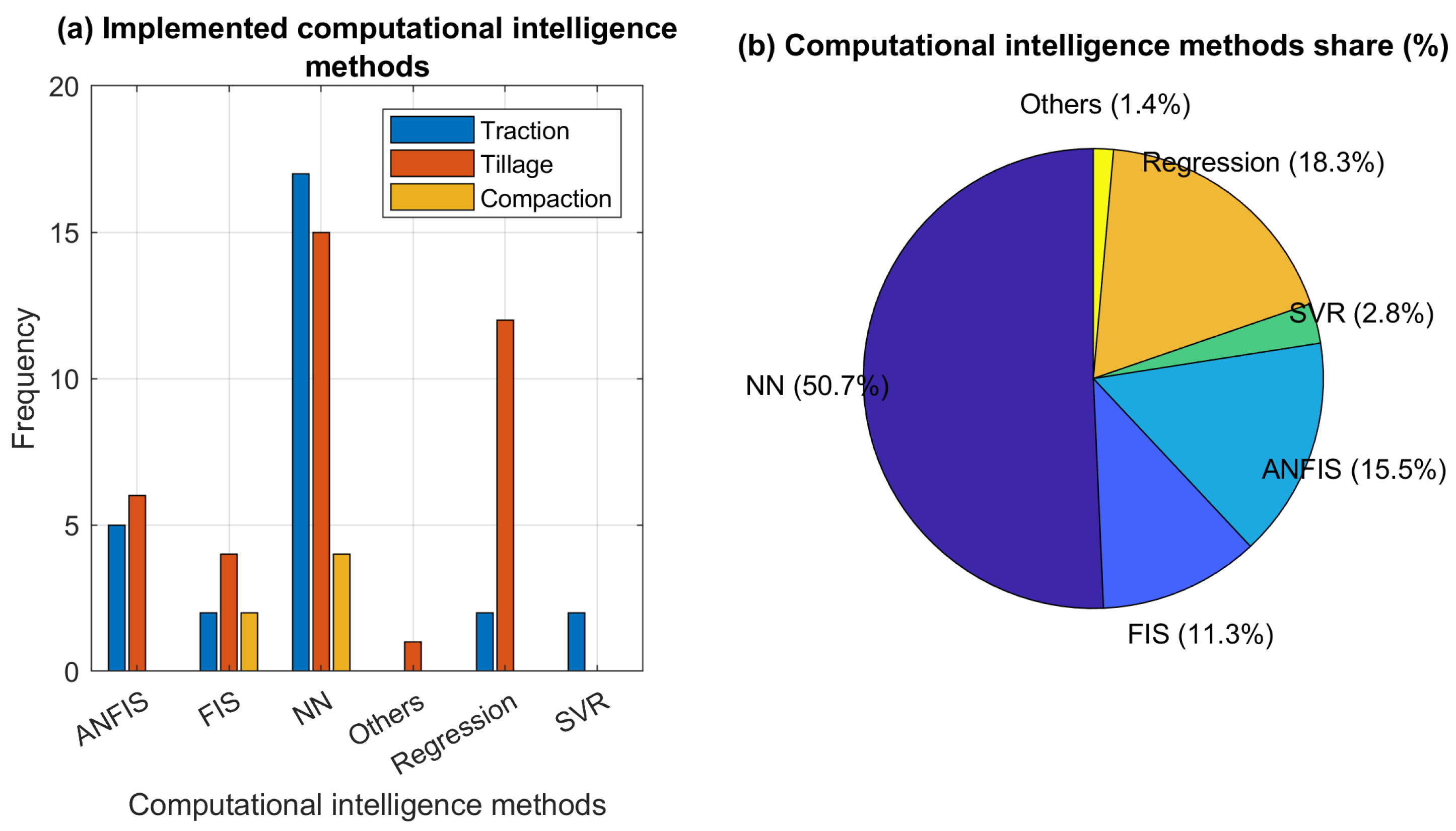
5.5. Implemented CI Methods

A summary of CI methods proposed in a selected article (50) is presented in Figure 15. The NNs were the most frequently employed, followed by multiple linear regression, ANFIS, and FIS. The NN-based models were proposed in 36 studies (50.7%), out of which 34 studies employed a fully connected feedforward (FF) NN type (Figure 15b). Other types of NNs, such as RNNs, wavelet NNs, and RBFNs, were reported once (Figure 16a). This indicates that shallow NN with only one or two layers was sufficient to model complex soil–machine interactions (Figure 16a). In most of these studies, NNs were trained with BP or LMBP (Figure 16b). A GA-based metaheuristic was used in one such research, and dimension reduction using ICA in another.

Subsequently, the FIS was implemented in a total of eight studies (11.3%). The triangular, Gaussian, and linear were observed as the most popular membership functions. The ANFIS models were proposed in eleven studies (15.5%), with the first-order TSK fuzzy inference system being the preferred approach. ANFIS models were often trained using a combination of the least-squares method and BP. The SVR models were applied in two studies, which used various kernel functions.

Additionally, traditional regression methods were implemented in thirteen (11.3%) studies. These regression methods included MLR and the standard ASABE equations (tool draft equation). These methods were usually compared with CI methods in terms of prediction accuracy.

The performances of the models were evaluated with commonly used metrics. Figure 17a shows the frequencies of their usages. As is evident from Figure 17b, CI models consistently outperformed classical approaches. Although the performance of the traditional regression method was comparatively lower in terms of model accuracy, MATLAB was the most widely used platform to implement CI-based models (Figure 17c).

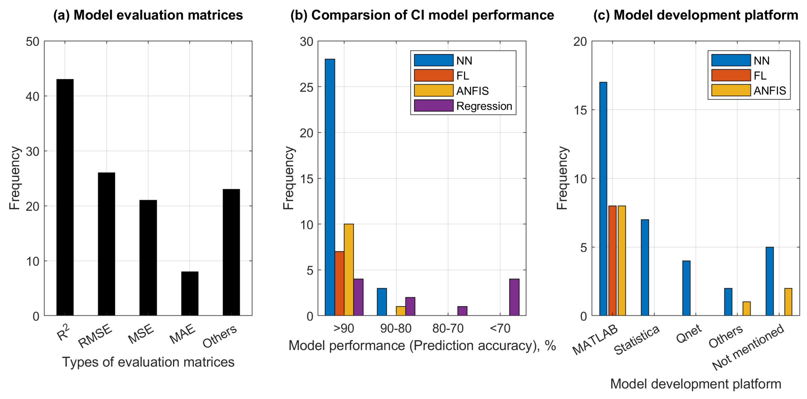
6. Strengths and Limitations of CI Methods

CI models offer manifold advantages over traditional methods described earlier. The features that make these models so attractive are enumerated below.

(i)

Data-driven models can handle copious amounts of data with relative ease [152]. With increasing data size, the corresponding growth in computational overheads is generally between linear and quadratic orders of magnitude. For instance, the number of iterations (called epochs) needed to train a neural network is fixed regardless of data size [53]. On the other hand, traditional methods regularly witness quadratic or higher growths.

(ii)

To further enhance their performances after initial offline training, data-driven CI models (e.g., NNs and DNNs) can learn online during actual deployment [153]. In other words, they are capable of learning from experience.

(iii)

FIS models can directly benefit from human domain experts; their expert knowledge can be incorporated into the model [154].

(iv)

Conversely, FIS model outputs are amenable to direct human interpretation. NNs endowed with such capability have been recently proposed [155].

(v)

CI-based algorithms can easily be hybridized with traditional algorithms as well as with one another, thereby offering the benefits of both (c.f. [48,156]). For instance, ANFIS is a combination of FIS and NN approaches.

(vi)

These models offer the advantage of flexibility. A model developed for a specific task can be adapted to handle another similar task [157,158].

(vii)

CI models are robust to various forms of imprecision, such as incomplete information, noise, and statistical outliers [152,159,160,161]. In some cases, they may even benefit from the presence of noise.

It is of little surprise that CI approaches have become very popular in agricultural soil-tillage, traction domains, and many other applications.

In spite of the several attractive features that CI models offer, they have a few shortcomings as well. These are outlined below.

(i)

Interpretability: Several CI models such as NN & SVR are black box approaches. Unlike physics-based approaches, the nonlinear input-output relationships expressed by these models are not self-explanatory, i.e., do not render themselves to common sense interpretations. Although various schemes towards making these relationships more explainable are currently being explored, [162,163,164,165], this research is only at a preliminary stage.

(ii)

Computational requirements: The development of CI models often requires specialized software (e.g., MATLAB). Moreover, training DNNs with reasonably sized data may prove to be too time-consuming unless using GPUs (graphics processing units), where processors can be run as a pipeline or in parallel [166].

(iii)

Data requirements: In comparison to classical methods, CI models require relatively copious amounts of data for training. As such models are not equipped for extrapolation, data samples must adequately cover the entire input range of real-world inputs. In order to effectively train certain CI models such as RBFNs, the data should not be skewed in any direction. Unfortunately, experimentally generating such data can often be a resource-intensive and time-consuming process.

(iv)

Output dimensionality: Unlike NNs, some other CI models are equipped to handle only scalar outputs. Although there are indirect methods to train SVRs with vector outputs [167,168], this is an inherent limitation of FIS models.

7. Emergent Computational Intelligence Models

The study critically analyzed the most popular CI methods found in the literature, particularly in the soil–machine interaction domain. Further, we suggest emergent CI methods that may provide better results and can be considered as alternatives to existing CI methods. Those methods are described in brief here.

7.1. Deep Neural Networks

DNNs are NN models with multiple hidden layers [169,170,171]. In the past few years, this class of CI models has witnessed explosive growth in popularity. DDNs have emerged as a popular tool in a wide range of applications in agriculture [172,173,174,175,176,177], where they have been used for various image recognition tasks. Unfortunately, DNNs have yet to be explored in any soil–machine interaction application.

Figure 4 illustrates the layout of such a DNN with fully connected layers. State-of-the-art DNNs incorporate various other types of layers, including RBFN [178], SVR [179], and TSK fuzzy [180,181] layers. DNNs can be endowed with the ability to handle time series data by incorporating long short-term memory (LSTM) or gated recurrent unit (GRU) layers [176,182]. At each time step t, these layers can hold in memory essential features from earlier time steps (i.e., $t-1$, $t-2$, etc.) by means of time-delayed feedback. Such DNNs are called recurrent neural networks. An alternate to LSTM and GRU in DNNs is the attention mechanism [183], which has been applied in agriculture [184].

Although sigmoid functions are widely used as neuronal nonlinearities, the presence of a large number of layers in the DNN poses the problem of vanishing gradients [185]. This issue is addressed by using rectified linear (ReLu) units [186], which incorporate the ReLu function, $f\left(s\right)=max(s,0).$ Current training methods that are based on BP [187,188,189]. The Adam (adaptive momentum estimation) algorithm is currently the dominant approach to train DNNs [190]. In [191], Adam was used to successfully train DNNs for agriculture data. The use of metaheuristics in conjunction with gradient methods has been investigated [192,193].

Unlike FIS and ANFIS models, DNNs are black-box approaches, whose outputs are not readily amenable to human interpretation. However, recent studies are beginning to address this issue [164,165].

7.2. Regression Trees and Random Forests

Decision trees are CI methods that use graphical tree-based representations [194,195], with binary trees [196] being most frequently used. During training, each node in a binary tree is used to split sample pairs $\left(\mathbf{x}\left(n\right),t\left(n\right)\right)$ ($n\in {\mathcal{S}}_t$) into two subsets ${\mathcal{S}}_t^{\mathrm{L}}$ and ${\mathcal{S}}_t^{\mathrm{LR}}$. A threshold ${\theta }_j$ is applied to an element $x_j$. Hence,

$$y=\left\{\begin{array}{c}{\mathcal{S}}_t^{\mathrm{L}}=\{n\in {\mathcal{S}}_t|x_j\left(n\right)\le {\theta }_j\};\hfill \\ {\mathcal{S}}_t^{\mathrm{R}}=\{n\in {\mathcal{S}}_t|x_j\left(n\right)>{\theta }_j\}.\hfill \end{array}\right.$$

(35)

The threshold is computed so that at each node, the split is as evenly balanced as possible. Information theoretic and heuristic methods using values of the targets $t\left(n\right)$ in the training dataset. Regression trees have found agricultural applications in the past few years [197,198].

Random forests are CI methods that use multiple trees to obtain outputs [199,200]. There has been a steep rise in the use of this approach for various applications in agriculture [201,202,203,204,205,206,207,208,209,210,211]. An excellent survey of decision trees, random forests, and other CI models has been published in [212].

7.3. Extreme Learning Machines

Extreme learning machines (ELM) are CI models that are useful in regression problems [213,214,215]. Although in comparison to some other CI models (NNs, RBFNs, and SVRs), ELMs have not been as widely used in other engineering domains; surprisingly, they are very popular in various agricultural applications [216,217,218,219,220,221,222,223].

An ELM is structurally equivalent to an $M\times K\times N$ NN. The neurons in the hidden layer incorporate nonlinear activation functions in the same manner as in Equation (9). However, unlike in NNs, the hidden layer in an ELM is not fully connected to the input. The hidden weights of an ELM can be arranged as a $K\times M$ sparse matrix. These weights are assigned randomly and do not undergo any training. Only the output weights are trained using a matrix form of the pseudoinverse rule in Equation (16). This allows ELMs to be trained significantly faster than equivalent NNs. Hybrid training algorithms for ELMs have also been proposed in [224,225,226] for agricultural applications. DNN architectures that contain ELM layers are being investigated (cf. [227,228]).

7.4. Bayesian Methods

Bayesian methods are CI paradigms where the outcome renders itself to a probabilistic interpretation. Central to these methods is the Bayes rule. The rule can be applied to a parametric Bayesian model in the following manner,

$$\mathrm{p}\left(\Theta |{\mathcal{S}}_t\right)=\frac{\mathrm{p}\left({\mathcal{S}}_t|\Theta \right)\mathrm{p}\left(\Theta \right)}{\mathrm{p}\left({\mathcal{S}}_t\right)}.$$

(36)

In this expression, $\mathrm{p}\left(·\right)$ is the probability of the argument. The left-hand side of Equation (36) is the posterior probability. The factors $\mathrm{p}\left({\mathcal{S}}_t|\Theta \right)$, and $\mathrm{p}\left({\mathcal{S}}_t\right)$ in the right-hand side are the likelihood and the prior probability. It can be demonstrated that LASSO and ridge regularization discussed earlier in Section 3.3 are instances of Bayesian methods, where the prior probabilities follow Laplacian and Gaussian distributions.

Since the training data ${\mathcal{S}}_t$ is independent of the model, it can be dropped from the Bayes rule. The model parameter is obtained as the one that has the highest probability, ${\mathrm{argmax}}_{\Theta }\mathrm{p}\left(\Theta |{\mathcal{S}}_t\right)$. Given any unknown input $\mathbf{x}$, the output probability $\mathrm{p}\left(y|\mathbf{x},\Theta \right)$ can be obtained from $\Theta$. Bayesian approaches have been used in several areas of agriculture [229,230,231,232].

A Bayesian network is a specific Bayesian modeling approach that uses a graphical structure that resembles an NN [233]. Inferring the output in this model relies heavily on statistical sampling techniques [234]. Bayesian networks have been used in [184,235,236].

A mixture of Gaussians [237,238] is a Bayesian model that uses hidden variables $z_i,i=1,2,\cdots$, which play an intermediate role between the inputs and outputs. Given any input $\mathbf{x}$, the output probability $\mathrm{p}\left(y\right)$ is determined as the following summation,

$$\mathrm{p}\left(y\right)=\sum _i\mathrm{p}\left(y\right|z_i)\mathrm{p}\left(z_i\right|\mathbf{x}).$$

(37)

The use of such methods has begun to be explored in agriculture [38,239,240].

Gaussian process regression [241,242,243] is a Bayesian approach that assumes the presence of Gaussian noise. As in SVR, kernel matrices are applied in this method. Gaussian process regression has been extensively used in various applications related to agriculture [244,245,246,247,248].

7.5. Ensemble Models

Ensemble models are approaches that combine multiple CI models for decision-making [249,250,251]. Bagging and boosting are two commonly used ensemble approaches. Random forests and Gaussian mixtures discussed earlier in this section are ensemble models.

There has been a surge in the use of these methods in the agriculture domain [252,253,254,255,256,257,258,259]. Recent research has been directed towards using bagging [260,261,262,263] and boosting [198]. Ensembles of NNs have been investigated in [264,265,266,267,268,269,270]. GA and PSO have also been studied in this context [255,264].

8. Future Direction and Scope

8.1. Online Traction Control

A sensing technology has reached its maturity, and ample research material is available, where numerous sensors were employed to sense, measure, and provide real-time information on the biological material (e.g., plant, soil, and field conditions). This review article taught us that CI methods can accurately and precisely model or predict complex soil–machine interactions. Therefore, future research efforts should target automatic and real-time traction-tillage control with the help of a sensing and prediction model. The online traction control system would optimize the machine parameters in real-time to increase traction efficiencies and reduce soil compaction. For example, traction control is a standard safety feature in today’s automotive vehicles. The wheel sensor senses the road conditions (icy or slippery), and the control algorithm enables the traction control to adapt to road conditions in real-time. Moreover, the planetary rover developed by NASA is also equipped with a traction control algorithm that senses the terrain driving condition and predicts the chance of getting trapped in soil (immobility condition) [271,272].

8.2. Online Tillage Control

The agricultural soil and field conditions are dynamic and vary on a spatial and temporal scale. Hence, a single tillage tool or management system operating uniformly throughout the field would not be sufficing. Multiple factors, including soil type, texture, structure, moisture, field topography, slope, and crop rotation, play a vital role when deciding which implement is best for the field. The current tillage management approach involves employing a single tillage tool for the entire area. The soil moisture is the only parameter checked before performing the tillage operation. Therefore, future research should develop variable depth, variable-intensity, and adaptive tillage implements that can be controlled in real-time. This site-specific tillage management would collect real-time information on soil and operating terrain, and CI models would serve as decision-support tools, creating a fully automated tillage management system. Site-specific tillage has excellent potential since the intensity of the operation is adapted to the local needs, which can dramatically improve tillage. Recently, adaptive tillage has become a significant research focus, where the tillage tool adapts or changes its shape in real-time [273,274].

References

1. Ani, O.A.; Uzoejinwa, B.; Ezeama, A.; Onwualu, A.; Ugwu, S.; Ohagwu, C. Overview of soil-machine interaction studies in soil bins. Soil Tillage Res. 2018, 175, 13–27. [Google Scholar] [CrossRef]
2. ASABE. Terminology and Definitions for Soil Tillage and Soil-Tool Relationships; Technical Report ASAE EP291.3 Feb2005 (R2018); American Society of Agricultural and Biological Engineers: St. Joseph, MI, USA, 2018. [Google Scholar]
3. Sunusi, I.I.; Zhou, J.; Zhen Wang, Z.; Sun, C.; Eltayeb Ibrahim, I.; Opiyo, S.; korohou, T.; Ahmed Soomro, S.; Alhaji Sale, N.; Olanrewaju, T.O. Intelligent tractors: Review of online traction control process. Comput. Electron. Agric. 2020, 170, 105176. [Google Scholar] [CrossRef]
4. Zoz, F.; Grisso, R. Traction and Tractor Performance; American Society of Agricultural and Biological Engineers: St. Joseph, MI, USA, 2012. [Google Scholar]
5. Upadhyaya, S.K.; Way, T.R.; Upadhyaya, S.K.; Chancellor, W.J. Chapter 2. Traction Mechanics. Part V. Traction Prediction Equations. In Advances in Soil Dynamics Volume 3, 1st ed.; American Society of Agricultural and Biological Engineers: St. Joseph, MI, USA, 2009; pp. 161–186. [Google Scholar] [CrossRef]
6. Karmakar, S.; Kushwaha, R.L. Dynamic modeling of soil–tool interaction: An overview from a fluid flow perspective. J. Terramech. 2006, 43, 411–425. [Google Scholar] [CrossRef]
7. Johnson, C.E.; Bailey, A.C. Soil Compaction. In Advances in Soil Dynamics Volume 2, 1st ed.; American Society of Agricultural and Biological Engineers: St. Joseph, MI, USA, 2002; pp. 155–178. [Google Scholar] [CrossRef] [Green Version]
8. Acquah, K.; Chen, Y. Soil Compaction from Wheel Traffic under Three Tillage Systems. Agriculture 2022, 12, 219. [Google Scholar] [CrossRef]
9. Soane, B.; van Ouwerkerk, C. Soil Compaction Problems in World Agriculture. In Developments in Agricultural Engineering; Elsevier: Amsterdam, The Netherlands, 1994; Volume 11, pp. 1–21. [Google Scholar] [CrossRef]
10. Brus, D.J.; van den Akker, J.J.H. How serious a problem is subsoil compaction in the Netherlands? A survey based on probability sampling. Soil 2018, 4, 37–45. [Google Scholar] [CrossRef] [Green Version]
11. Zabrodskyi, A.; Šarauskis, E.; Kukharets, S.; Juostas, A.; Vasiliauskas, G.; Andriušis, A. Analysis of the Impact of Soil Compaction on the Environment and Agricultural Economic Losses in Lithuania and Ukraine. Sustainability 2021, 13, 7762. [Google Scholar] [CrossRef]
12. Keller, T. Soil Compaction and Soil Tillage—Studies in Agricultural Soil Mechanics. Ph.D. Thesis, Swedish University of Agricultural Sciences, Uppsala, Sweden, 2004. [Google Scholar]
13. DeJong-Hughes, J.; Moncrief, J.; Voorhees, W.; Swan, J. Soil Compaction: Causes, Effects and Control; The University of Minnesota Extension Service: St. Paul, MN, USA, 2001; Available online: https://hdl.handle.net/11299/55483 (accessed on 24 October 2022).
14. Badalíková, B. Influence of Soil Tillage on Soil Compaction. In Soil Engineering; Dedousis, A.P., Bartzanas, T., Eds.; Springer: Berlin/Heidelberg, Germany, 2010; Volume 20, pp. 19–30. [Google Scholar] [CrossRef]
15. Tiwari, V.; Pandey, K.; Pranav, P. A review on traction prediction equations. J. Terramechan. 2010, 47, 191–199. [Google Scholar] [CrossRef]
16. Wong, J.Y. Theory of Ground Vehicles, 3rd ed.; John Wiley: New York, NY, USA, 2001. [Google Scholar]
17. Godwin, R.; Spoor, G. Soil failure with narrow tines. J. Agric. Eng. Res. 1977, 22, 213–228. [Google Scholar] [CrossRef]
18. Makanga, J.; Salokhe, V.; Gee-Clough, D. Effect of tine rake angle and aspect ratio on soil failure patterns in dry loam soil. J. Terramech. 1996, 33, 233–252. [Google Scholar] [CrossRef]
19. Karmakar, S. Numerical Modeling of Soil Flow and Pressure Distribution on a Simple Tillage Tool Using Computational Fluid Dynamics. Ph.D. Thesis, University of Saskatchewan, Saskatoon, SK, Canada, 2005. [Google Scholar]
20. Tagar, A.; Ji, C.; Ding, Q.; Adamowski, J.; Chandio, F.; Mari, I. Soil failure patterns and draft as influenced by consistency limits: An evaluation of the remolded soil cutting test. Soil Tillage Res. 2014, 137, 58–66. [Google Scholar] [CrossRef]
21. Roul, A.; Raheman, H.; Pansare, M.; Machavaram, R. Predicting the draught requirement of tillage implements in sandy clay loam soil using an artificial neural network. Biosyst. Eng. 2009, 104, 476–485. [Google Scholar] [CrossRef]
22. Fielke, J.; Riley, T. The universal earthmoving equation applied to chisel plough wings. J. Terramech. 1991, 28, 11–19. [Google Scholar] [CrossRef]
23. Godwin, R.; Seig, D.; Allott, M. Soil failure and force prediction for soil engaging discs. Soil Use Manag. 1987, 3, 106–114. [Google Scholar] [CrossRef]
24. Kushwaha, R.L.; Shen, J. Finite Element Analysis of the Dynamic Interaction Between Soil and Tillage Tool. Trans. ASAE 1995, 38, 1315–1319. [Google Scholar] [CrossRef]
25. Upadhyaya, S.K.; Rosa, U.A.; Wulfsohn, D. Application of the Finite Element Method in Agricultural Soil Mechanics. In Advances in Soil Dynamics Volume 2, 1st ed.; American Society of Agricultural and Biological Engineers: St. Joseph, MI, USA, 2002; pp. 117–153. [Google Scholar] [CrossRef]
26. Shmulevich, I.; Rubinstein, D.; Asaf, Z. Chapter 5. Discrete Element Modeling of Soil-Machine Interactions. In Advances in Soil Dynamics Volume 3, 1st ed.; American Society of Agricultural and Biological Engineers: St. Joseph, MI, USA, 2009; pp. 399–433. [Google Scholar] [CrossRef]
27. Liu, J.; Kushwaha, R.L. Two-decade Achievements in Modeling of Soil—Tool Interactions. In Proceedings of the ASABE Annual International Meeting 2008, Providence, RI, USA, 29 June–2 July 2008; American Society of Agricultural and Biological Engineers: St. Joseph, MI, USA, 2008. [Google Scholar] [CrossRef]
28. Taheri, S.; Sandu, C.; Taheri, S.; Pinto, E.; Gorsich, D. A technical survey on Terramechanics models for tire–terrain interaction used in modeling and simulation of wheeled vehicles. J. Terramech. 2015, 57, 1–22. [Google Scholar] [CrossRef]
29. Ghosh, S.; Konar, A. An Overview of Computational Intelligence Algorithms. In Call Admission Control in Mobile Cellular Networks; Springer: Berlin/Heidelberg, Germany, 2013; pp. 63–94. [Google Scholar] [CrossRef]
30. Vasant, P. Handbook of Research on Novel Soft Computing Intelligent Algorithms: Theory and Practical Applications; IGI Global: Hershey, PA, USA, 2013. [Google Scholar] [CrossRef]
31. Xing, B.; Gao, W.J. Innovative Computational Intelligence: A Rough Guide to 134 Clever Algorithms; Springer: Manhattan, NY, USA, 2014; Volume 62. [Google Scholar]
32. Ibrahim, D. An overview of soft computing. Procedia Comput. Sci. 2016, 102, 34–38. [Google Scholar] [CrossRef] [Green Version]
33. Ding, S.; Li, H.; Su, C.; Yu, J.; Jin, F. Evolutionary artificial neural networks: A review. Artif. Intell. Rev. 2013, 39, 251–260. [Google Scholar] [CrossRef]
34. Stanley, K.O.; Clune, J.; Lehman, J.; Miikkulainen, R. Designing neural networks through neuroevolution. Nat. Mach. Intell. 2019, 1, 24–35. [Google Scholar] [CrossRef] [Green Version]
35. Elbes, M.; Alzubi, S.; Kanan, T.; Al-Fuqaha, A.; Hawashin, B. A survey on particle swarm optimization with emphasis on engineering and network applications. Evol. Intell. 2019, 12, 113–129. [Google Scholar] [CrossRef]
36. Karaboga, D.; Kaya, E. Adaptive network based fuzzy inference system (ANFIS) training approaches: A comprehensive survey. Artif. Intell. Rev. 2019, 52, 2263–2293. [Google Scholar] [CrossRef]
37. Ridzuan, F.; Zainon, W.M.N.W. A review on data cleansing methods for big data. Procedia Comput. Sci. 2019, 161, 731–738. [Google Scholar] [CrossRef]
38. Badgujar, C.; Das, S.; Flippo, D.; Welch, S.M.; Martinez-Figueroa, D. A Deep Neural Network-Based Approach to Predict the Traction, Mobility, and Energy Consumption of Autonomous Ground Vehicle on Sloping Terrain Field. Comput. Electron. Agric. 2022, 196, 106867. [Google Scholar] [CrossRef]
39. Scholz, M. Validation of nonlinear PCA. Neural Process. Lett. 2012, 36, 21–30. [Google Scholar] [CrossRef]
40. Stone, J.V. Independent component analysis: An introduction. Trends Cogn. Sci. 2002, 6, 59–64. [Google Scholar] [CrossRef] [PubMed]
41. Cherkassky, V.; Ma, Y. Comparison of loss functions for linear regression. In Proceedings of the 2004 IEEE International Joint Conference on Neural Networks, Budapest, Hungary, 25–29 July 2004; Volume 1, pp. 395–400. [Google Scholar] [CrossRef]
42. Čížek, P.; Sadıkoğlu, S. Robust nonparametric regression: A review. Wiley Interdiscip. Rev. Comput. Stat. 2020, 12, e1492. [Google Scholar] [CrossRef] [Green Version]
43. Huang, S.; Wu, Q. Robust pairwise learning with Huber loss. J. Complex. 2021, 66, 101570. [Google Scholar] [CrossRef]
44. Vapnik, V.; Levin, E.; Le Cun, Y. Measuring the VC-dimension of a learning machine. Neural Comput. 1994, 6, 851–876. [Google Scholar] [CrossRef]
45. Zou, H.; Hastie, T. Regularization and variable selection via the elastic net. J. R. Stat. Soc. Ser. B (Stat. Methodol.) 2005, 67, 301–320. [Google Scholar] [CrossRef] [Green Version]
46. Wilamowski, B.M.; Yu, H. Improved computation for Levenberg–Marquardt training. IEEE Trans. Neural Netw. 2010, 21, 930–937. [Google Scholar] [CrossRef] [PubMed]
47. Rodriguez, J.D.; Perez, A.; Lozano, J.A. Sensitivity analysis of k-fold cross validation in prediction error estimation. IEEE Trans. Pattern Anal. Mach. Intell. 2009, 32, 569–575. [Google Scholar] [CrossRef] [PubMed]
48. Das, S.; Koduru, P.; Gui, M.; Cochran, M.; Wareing, A.; Welch, S.M.; Babin, B.R. Adding local search to particle swarm optimization. In Proceedings of the 2006 IEEE International Conference on Evolutionary Computation, Vancouver, BC, Canada, 16–21 July 2006; pp. 428–433. [Google Scholar]
49. Taghavifar, H.; Mardani, A. Energy loss optimization of run-off-road wheels applying imperialist competitive algorithm. Inf. Process. Agric. 2014, 1, 57–65. [Google Scholar] [CrossRef] [Green Version]
50. Taghavifar, H.; Mardani, A. Evaluating the effect of tire parameters on required drawbar pull energy model using adaptive neuro-fuzzy inference system. Energy 2015, 85, 586–593. [Google Scholar] [CrossRef]
51. Rumelhart, D.E.; Hinton, G.E.; Williams, R.J. Learning representations by back-propagating errors. Nature 1986, 323, 533–536. [Google Scholar] [CrossRef]
52. Sapna, S.; Tamilarasi, A.; Kumar, M.P. Backpropagation learning algorithm based on Levenberg Marquardt Algorithm. Comput. Sci. Inf. Technol. (CS IT) 2012, 2, 393–398. [Google Scholar]
53. Abu-Mostafa, Y.S.; Magdon-Ismail, M.; Lin, H.T. Learning from Data; AMLBook: New York, NY, USA, 2012. [Google Scholar]
54. Ghosh, J.; Nag, A. An overview of radial basis function networks. In Radial Basis Function Networks 2; Springer: New York, NY, USA, 2001; pp. 1–36. [Google Scholar]
55. Ruß, G. Data mining of agricultural yield data: A comparison of regression models. In Proceedings of the Industrial Conference on Data Mining, Leipzig, Germany, 20–22 July 2009; Springer: New York, NY, USA, 2009; pp. 24–37. [Google Scholar]
56. da Silva, E.M., Jr.; Maia, R.D.; Cabacinha, C.D. Bee-inspired RBF network for volume estimation of individual trees. Comput. Electron. Agric. 2018, 152, 401–408. [Google Scholar] [CrossRef]
57. Zhang, D.; Zang, G.; Li, J.; Ma, K.; Liu, H. Prediction of soybean price in China using QR-RBF neural network model. Comput. Electron. Agric. 2018, 154, 10–17. [Google Scholar] [CrossRef]
58. Ashraf, T.; Khan, Y.N. Weed density classification in rice crop using computer vision. Comput. Electron. Agric. 2020, 175, 105590. [Google Scholar] [CrossRef]
59. Eide, Å.J.; Lindblad, T.; Paillet, G. Radial-basis-function networks. In Intelligent Systems; CRC Press: Boca Raton, FL, USA, 2018. [Google Scholar]
60. Bock, H.H. Clustering methods: A history of k-means algorithms. Selected Contributions in Data Analysis and Classification; Springer: New York, NY, USA, 2007; pp. 161–172. [Google Scholar]
61. Smola, A.J.; Schölkopf, B. A tutorial on support vector regression. Stat. Comput. 2004, 14, 199–222. [Google Scholar] [CrossRef] [Green Version]
62. Pisner, D.A.; Schnyer, D.M. Support vector machine. In Machine learning; Elsevier: Amsterdam, The Netherlands, 2020; pp. 101–121. [Google Scholar]
63. Cervantes, J.; Garcia-Lamont, F.; Rodríguez-Mazahua, L.; Lopez, A. A comprehensive survey on support vector machine classification: Applications, challenges and trends. Neurocomputing 2020, 408, 189–215. [Google Scholar] [CrossRef]
64. Mucherino, A.; Papajorgji, P.; Pardalos, P.M. A survey of data mining techniques applied to agriculture. Oper. Res. 2009, 9, 121–140. [Google Scholar] [CrossRef]
65. Mehdizadeh, S.; Behmanesh, J.; Khalili, K. Using MARS, SVM, GEP and empirical equations for estimation of monthly mean reference evapotranspiration. Comput. Electron. Agric. 2017, 139, 103–114. [Google Scholar] [CrossRef]
66. Patrício, D.I.; Rieder, R. Computer vision and artificial intelligence in precision agriculture for grain crops: A systematic review. Comput. Electron. Agric. 2018, 153, 69–81. [Google Scholar] [CrossRef] [Green Version]
67. Kok, Z.H.; Shariff, A.R.M.; Alfatni, M.S.M.; Khairunniza-Bejo, S. Support vector machine in precision agriculture: A review. Comput. Electron. Agric. 2021, 191, 106546. [Google Scholar] [CrossRef]
68. Burges, C.J. A tutorial on support vector machines for pattern recognition. Data Min. Knowl. Discov. 1998, 2, 121–167. [Google Scholar] [CrossRef]
69. Hindi, H. A tutorial on convex optimization. In Proceedings of the 2004 American Control Conference, Boston, MA, USA, 30 June–2 July 2004; Volume 4, pp. 3252–3265. [Google Scholar]
70. Hindi, H. A tutorial on convex optimization II: Duality and interior point methods. In Proceedings of the 2006 American Control Conference, Minneapolis, MN, USA, 14–16 June 2006; p. 11. [Google Scholar]
71. Chapelle, O. Training a support vector machine in the primal. Neural Comput. 2007, 19, 1155–1178. [Google Scholar] [CrossRef] [Green Version]
72. Liang, Z.; Li, Y. Incremental support vector machine learning in the primal and applications. Neurocomputing 2009, 72, 2249–2258. [Google Scholar] [CrossRef]
73. Wu, J.; Wang, Y.G. Iterative Learning in Support Vector Regression with Heterogeneous Variances. IEEE Trans. Emerg. Top. Comput. Intell. 2022, 1–10. [Google Scholar] [CrossRef]
74. Zimmermann, H.J. Fuzzy set theory. Wiley Interdiscip. Rev. Comput. Stat. 2010, 2, 317–332. [Google Scholar] [CrossRef]
75. Iancu, I. A Mamdani type fuzzy logic controller. Fuzzy Log. -Control. Concepts Theor. Appl. 2012, 15, 325–350. [Google Scholar]
76. Guerra, T.M.; Kruszewski, A.; Lauber, J. Discrete Tagaki–Sugeno models for control: Where are we? Annu. Rev. Control 2009, 33, 37–47. [Google Scholar] [CrossRef]
77. Nguyen, A.T.; Taniguchi, T.; Eciolaza, L.; Campos, V.; Palhares, R.; Sugeno, M. Fuzzy control systems: Past, present and future. IEEE Comput. Intell. Mag. 2019, 14, 56–68. [Google Scholar] [CrossRef]
78. Nakanishi, H.; Turksen, I.; Sugeno, M. A review and comparison of six reasoning methods. Fuzzy Sets Syst. 1993, 57, 257–294. [Google Scholar] [CrossRef]
79. Ying, H.; Ding, Y.; Li, S.; Shao, S. Comparison of necessary conditions for typical Takagi-Sugeno and Mamdani fuzzy systems as universal approximators. IEEE Trans. Syst. Man Cybern. -Part A Syst. Humans 1999, 29, 508–514. [Google Scholar] [CrossRef] [Green Version]
80. Huang, Y.; Lan, Y.; Thomson, S.J.; Fang, A.; Hoffmann, W.C.; Lacey, R.E. Development of soft computing and applications in agricultural and biological engineering. Comput. Electron. Agric. 2010, 71, 107–127. [Google Scholar] [CrossRef] [Green Version]
81. Touati, F.; Al-Hitmi, M.; Benhmed, K.; Tabish, R. A fuzzy logic based irrigation system enhanced with wireless data logging applied to the state of Qatar. Comput. Electron. Agric. 2013, 98, 233–241. [Google Scholar] [CrossRef]
82. Zareiforoush, H.; Minaei, S.; Alizadeh, M.R.; Banakar, A.; Samani, B.H. Design, development and performance evaluation of an automatic control system for rice whitening machine based on computer vision and fuzzy logic. Comput. Electron. Agric. 2016, 124, 14–22. [Google Scholar] [CrossRef]
83. Kisi, O.; Sanikhani, H.; Zounemat-Kermani, M.; Niazi, F. Long-term monthly evapotranspiration modeling by several data-driven methods without climatic data. Comput. Electron. Agric. 2015, 115, 66–77. [Google Scholar] [CrossRef]
84. Valdés-Vela, M.; Abrisqueta, I.; Conejero, W.; Vera, J.; Ruiz-Sánchez, M.C. Soft computing applied to stem water potential estimation: A fuzzy rule based approach. Comput. Electron. Agric. 2015, 115, 150–160. [Google Scholar] [CrossRef]
85. Malik, A.; Kumar, A.; Piri, J. Daily suspended sediment concentration simulation using hydrological data of Pranhita River Basin, India. Comput. Electron. Agric. 2017, 138, 20–28. [Google Scholar] [CrossRef]
86. Shafaei, S.; Loghavi, M.; Kamgar, S. Appraisal of Takagi-Sugeno-Kang type of adaptive neuro-fuzzy inference system for draft force prediction of chisel plow implement. Comput. Electron. Agric. 2017, 142, 406–415. [Google Scholar] [CrossRef]
87. Shiri, J.; Keshavarzi, A.; Kisi, O.; Iturraran-Viveros, U.; Bagherzadeh, A.; Mousavi, R.; Karimi, S. Modeling soil cation exchange capacity using soil parameters: Assessing the heuristic models. Comput. Electron. Agric. 2017, 135, 242–251. [Google Scholar] [CrossRef]
88. Jang, J.S.; Sun, C.T. Neuro-fuzzy modeling and control. Proc. IEEE 1995, 83, 378–406. [Google Scholar] [CrossRef]
89. Babuška, R.; Verbruggen, H. Neuro-fuzzy methods for nonlinear system identification. Annu. Rev. Control 2003, 27, 73–85. [Google Scholar] [CrossRef]
90. Shihabudheen, K.; Pillai, G.N. Recent advances in neuro-fuzzy system: A survey. Knowl.-Based Syst. 2018, 152, 136–162. [Google Scholar] [CrossRef]
91. de Campos Souza, P.V. Fuzzy neural networks and neuro-fuzzy networks: A review the main techniques and applications used in the literature. Appl. Soft Comput. 2020, 92, 106275. [Google Scholar] [CrossRef]
92. Wu, W.; Li, L.; Yang, J.; Liu, Y. A modified gradient-based neuro-fuzzy learning algorithm and its convergence. Inf. Sci. 2010, 180, 1630–1642. [Google Scholar] [CrossRef]
93. Wang, L.; Zhang, H. An adaptive fuzzy hierarchical control for maintaining solar greenhouse temperature. Comput. Electron. Agric. 2018, 155, 251–256. [Google Scholar] [CrossRef]
94. Shafaei, S.; Loghavi, M.; Kamgar, S. An extensive validation of computer simulation frameworks for neural prognostication of tractor tractive efficiency. Comput. Electron. Agric. 2018, 155, 283–297. [Google Scholar] [CrossRef]
95. Petković, B.; Petković, D.; Kuzman, B.; Milovančević, M.; Wakil, K.; Ho, L.S.; Jermsittiparsert, K. Neuro-fuzzy estimation of reference crop evapotranspiration by neuro fuzzy logic based on weather conditions. Comput. Electron. Agric. 2020, 173, 105358. [Google Scholar] [CrossRef]
96. Wiktorowicz, K. RFIS: Regression-based fuzzy inference system. Neural Comput. Appl. 2022, 34, 12175–12196. [Google Scholar] [CrossRef]
97. Cheng, C.B.; Cheng, C.J.; Lee, E. Neuro-fuzzy and genetic algorithm in multiple response optimization. Comput. Math. Appl. 2002, 44, 1503–1514. [Google Scholar] [CrossRef] [Green Version]
98. Shihabudheen, K.; Mahesh, M.; Pillai, G.N. Particle swarm optimization based extreme learning neuro-fuzzy system for regression and classification. Expert Syst. Appl. 2018, 92, 474–484. [Google Scholar] [CrossRef]
99. Castellano, G.; Castiello, C.; Fanelli, A.M.; Jain, L. Evolutionary neuro-fuzzy systems and applications. In Advances in Evolutionary Computing for System Design; Springer: New York, NY, USA, 2007; pp. 11–45. [Google Scholar]
100. Aghelpour, P.; Bahrami-Pichaghchi, H.; Kisi, O. Comparison of three different bio-inspired algorithms to improve ability of neuro fuzzy approach in prediction of agricultural drought, based on three different indexes. Comput. Electron. Agric. 2020, 170, 105279. [Google Scholar] [CrossRef]
101. Hassan, A.; Tohmaz, A. Performance of Skidder Tires in Swamps—Comparison between Statistical and Neural Network Models. Trans. ASAE 1995, 38, 1545–1551. [Google Scholar] [CrossRef]
102. Taghavifar, H.; Mardani, A.; Hosseinloo, A.H. Appraisal of artificial neural network-genetic algorithm based model for prediction of the power provided by the agricultural tractors. Energy 2015, 93, 1704–1710. [Google Scholar] [CrossRef]
103. Shafaei, S.; Loghavi, M.; Kamgar, S. Benchmark of an intelligent fuzzy calculator for admissible estimation of drawbar pull supplied by mechanical front wheel drive tractor. Artif. Intell. Agric. 2020, 4, 209–218. [Google Scholar] [CrossRef]
104. Cutini, M.; Costa, C.; Brambilla, M.; Bisaglia, C. Relationship between the 3D Footprint of an Agricultural Tire and Drawbar Pull Using an Artificial Neural Network. Appl. Eng. Agric. 2022, 38, 293–301. [Google Scholar] [CrossRef]
105. American National Standard ANSI/ASAE S296.5 DEC2003 (R2018); General Terminology for Traction of Agricultural Traction and Transport Devices and Vehicles. ASABE: St. Joseph, MI, USA, 2018.
106. Carman, K.; Taner, A. Prediction of Tire Tractive Performance by Using Artificial Neural Networks. Math. Comput. Appl. 2012, 17, 182–192. [Google Scholar] [CrossRef] [Green Version]
107. Taghavifar, H.; Mardani, A. On the modeling of energy efficiency indices of agricultural tractor driving wheels applying adaptive neuro-fuzzy inference system. J. Terramech. 2014, 56, 37–47. [Google Scholar] [CrossRef]
108. Taghavifar, H.; Mardani, A. Applying a supervised ANN (artificial neural network) approach to the prognostication of driven wheel energy efficiency indices. Energy 2014, 68, 651–657. [Google Scholar] [CrossRef]
109. Taghavifar, H.; Mardani, A. Use of artificial neural networks for estimation of agricultural wheel traction force in soil bin. Neural Comput. Appl. 2014, 24, 1249–1258. [Google Scholar] [CrossRef]
110. Ekinci, S.; Carman, K.; Kahramanlı, H. Investigation and modeling of the tractive performance of radial tires using off-road vehicles. Energy 2015, 93, 1953–1963. [Google Scholar] [CrossRef]
111. Pentoś, K.; Pieczarka, K. Applying an artificial neural network approach to the analysis of tractive properties in changing soil conditions. Soil Tillage Res. 2017, 165, 113–120. [Google Scholar] [CrossRef]
112. Pentoś, K.; Pieczarka, K.; Lejman, K. Application of Soft Computing Techniques for the Analysis of Tractive Properties of a Low-Power Agricultural Tractor under Various Soil Conditions. Complexity 2020. [Google Scholar] [CrossRef]
113. Taghavifar, H.; Mardani, A.; Karim-Maslak, H.; Kalbkhani, H. Artificial Neural Network estimation of wheel rolling resistance in clay loam soil. Appl. Soft Comput. 2013, 13, 3544–3551. [Google Scholar] [CrossRef]
114. Taghavifar, H.; Mardani, A. A knowledge-based Mamdani fuzzy logic prediction of the motion resistance coefficient in a soil bin facility for clay loam soil. Neural Comput. Appl. 2013, 23, 293–302. [Google Scholar] [CrossRef]
115. Taghavifar, H.; Mardani, A. A comparative trend in forecasting ability of artificial neural networks and regressive support vector machine methodologies for energy dissipation modeling of off-road vehicles. Energy 2014, 66, 569–576. [Google Scholar] [CrossRef]
116. Almaliki, S.; Alimardani, R.; Omid, M. Artificial Neural Network Based Modeling of Tractor Performance at Different Field Conditions. Agric. Eng. Int. CIGR J. 2016, 18, 262–274. [Google Scholar]
117. Shafaei, S.; Loghavi, M.; Kamgar, S. Feasibility of implementation of intelligent simulation configurations based on data mining methodologies for prediction of tractor wheel slip. Inf. Process. Agric. 2019, 6, 183–199. [Google Scholar] [CrossRef]
118. Küçüksariyildiz, H.; Çarman, K.; Sabanci, K. Prediction of Specific Fuel Consumption of 60 HP 2WD Tractor Using Artificial Neural Networks. Int. J. Automot. Sci. Technol. 2021, 5, 436–444. [Google Scholar] [CrossRef]
119. Badgujar, C.; Flippo, D.; Welch, S. Artificial neural network to predict traction performance of autonomous ground vehicle on a sloped soil bin and uncertainty analysis. Comput. Electron. Agric. 2022, 196, 106867. [Google Scholar] [CrossRef]
120. Choi, Y.S.; Lee, K.S.; Park, W.Y. Application of a Neural Network to Dynamic Draft Model. Agric. Biosyst. Eng. 2000, 1, 67–72. [Google Scholar]
121. ASABE. Agricultural Machinery Management Data; Technical Report ASAE D497.4 MAR99; American Society of Agricultural and Biological Engineers (ASABE): St. Joseph, MI, USA, 2000. [Google Scholar]
122. Al-Janobi, A.; Al-Hamed, S.; Aboukarima, A.; Almajhadi, Y. Modeling of Draft and Energy Requirements of a Moldboard Plow Using Artificial Neural Networks Based on Two Novel Variables. Eng. Agrícola 2020, 40, 363–373. [Google Scholar] [CrossRef]
123. Shafaei, S.; Loghavi, M.; Kamgar, S.; Raoufat, M. Potential assessment of neuro-fuzzy strategy in prognostication of draft parameters of primary tillage implement. Ann. Agrar. Sci. 2018, 16, 257–266. [Google Scholar] [CrossRef]
124. Çarman, K.; Çıtıl, E.; Taner, A. Artificial Neural Network Model for Predicting Specific Draft Force and Fuel Consumption Requirement of a Mouldboard Plough. Selcuk J. Agric. Food Sci. 2019, 33, 241–247. [Google Scholar] [CrossRef]
125. Al-Hamed, S.A.; Wahby, M.F.; Al-Saqer, S.M.; Aboukarima, A.M.; Ahmed, A.S. Artificial neural network model for predicting draft and energy requirements of a disk plow. J. Anim. Plant Sci. 2013, 23, 1714–1724. [Google Scholar]
126. Shafaei, S.M.; Loghavi, M.; Kamgar, S. A comparative study between mathematical models and the ANN data mining technique in draft force prediction of disk plow implement in clay loam soil. Agric. Eng. Int. CIGR J. 2018, 20, 71–79. [Google Scholar]
127. Aboukarima, A.; Saad, A.F. Assessment of Different Indices Depicting Soil Texture for Predicting Chisel Plow Draft Using Neural Networks. Alex. Sci. Exch. J. 2006, 27, 170–180. [Google Scholar]
128. Marey, S.; Aboukarima, A.; Almajhadi, Y. Predicting the Performance Parameters of Chisel Plow Using Neural Network Model. Eng. Agrícola 2020, 40, 719–731. [Google Scholar] [CrossRef]
129. DeJong-Hughes, J. Tillage Implements, 2021; The University of Minnesota Extension Service: St. Paul, MN, USA, 2021. [Google Scholar]
130. Alimardani, R.; Abbaspour-Gilandeh, Y.; Khalilian, A.; Keyhani, A.; Sadati, S.H. Prediction of draft force and energy of subsoiling operation using ANN model. J. Food, Agric. Environ. 2009, 7, 537–542. [Google Scholar]
131. Bergtold, J.; Sailus, M.; Jackson, T. Conservation Tillage Systems in the Southeast: Production, Profitability and Stewardship; USDA: Washington, DC, USA; Sustainable Agriculture Research & Education: College Park, MD, USA, 2020. [Google Scholar]
132. Askari, M.; Abbaspour-Gilandeh, Y. Assessment of adaptive neuro-fuzzy inference system and response surface methodology approaches in draft force prediction of subsoiling tines. Soil Tillage Res. 2019, 194, 104338. [Google Scholar] [CrossRef]
133. Abbaspour-Gilandeh, M.; Shahgoli, G.; Abbaspour-Gilandeh, Y.; Herrera-Miranda, M.A.; Hernández-Hernández, J.L.; Herrera-Miranda, I. Measuring and Comparing Forces Acting on Moldboard Plow and Para-Plow with Wing to Replace Moldboard Plow with Para-Plow for Tillage and Modeling It Using Adaptive Neuro-Fuzzy Interface System (ANFIS). Agriculture 2020, 10, 633. [Google Scholar] [CrossRef]
134. Abbaspour-Gilandeh, Y.; Sedghi, R. Predicting soil fragmentation during tillage operation using fuzzy logic approach. J. Terramech. 2015, 57, 61–69. [Google Scholar] [CrossRef]
135. Marakoğlu, T.; Çarman, K. Fuzzy knowledge-based model for prediction of soil loosening and draft efficiency in tillage. J. Terramech. 2010, 47, 173–178. [Google Scholar] [CrossRef]
136. Abbaspour-Gilandeh, Y.; Fazeli, M.; Roshanianfard, A.; Hernández-Hernández, M.; Gallardo-Bernal, I.; Hernández-Hernández, J.L. Prediction of Draft Force of a Chisel Cultivator Using Artificial Neural Networks and Its Comparison with Regression Model. Agronomy 2020, 10, 451. [Google Scholar] [CrossRef] [Green Version]
137. Zhang, Z.X.; Kushwaha, R. Applications of neural networks to simulate soil-tool interaction and soil behavior. Can. Agric. Eng. 1999, 41, 119–125. [Google Scholar]
138. Mohammadi, A. Modeling of Draft Force Variation in a Winged Share Tillage Tool Using Fuzzy Table Look-Up Scheme. Agric. Eng. Int. CIGR J. 2012, 14, 262–268. [Google Scholar]
139. Akbarnia, A.; Mohammadi, A.; Alimardani, R.; Farhani, F. Simulation of draft force of winged share tillage tool using artificial neural network model. Agric. Eng. Int. CIGR J. 2014, 16, 57–65. [Google Scholar]
140. Usaborisut, P.; Prasertkan, K. Specific energy requirements and soil pulverization of a combined tillage implement. Heliyon 2019, 5, e02757. [Google Scholar] [CrossRef]
141. Upadhyay, G.; Raheman, H. Comparative assessment of energy requirement and tillage effectiveness of combined (active-passive) and conventional offset disc harrows. Biosyst. Eng. 2020, 198, 266–279. [Google Scholar] [CrossRef]
142. Shafaei, S.; Loghavi, M.; Kamgar, S. Prognostication of energy indices of tractor-implement utilizing soft computing techniques. Inf. Process. Agric. 2019, 6, 132–149. [Google Scholar] [CrossRef]
143. Rahman, A.; Kushwaha, R.L.; Ashrafizadeh, S.R.; Panigrahi, S. Prediction of Energy Requirement of a Tillage Tool in a Soil Bin using Artificial Neural Network. In Proceedings of the 2011 ASABE Annual International Meeting, Louisville, KY, USA, 7–10 August 2011; ASABE: St. Joseph, MI, USA, 2011. [Google Scholar] [CrossRef]
144. Saleh, B.; Aly, A. Artificial Neural Network Model for Evaluation of the Ploughing Process Performance. Int. J. Control Autom. Syst. 2013, 2, 1–11. [Google Scholar]
145. Shafaei, S.; Loghavi, M.; Kamgar, S. On the neurocomputing based intelligent simulation of tractor fuel efficiency parameters. Inf. Process. Agric. 2018, 5, 205–223. [Google Scholar] [CrossRef]
146. Shafaei, S.M.; Loghavi, M.; Kamgar, S. On the Reliability of Intelligent Fuzzy System for Multivariate Pattern Scrutinization of Power Consumption Efficiency of Mechanical Front Wheel Drive Tractor. J. Biosyst. Eng. 2021, 46, 1–15. [Google Scholar] [CrossRef]
147. Carman, K. Prediction of soil compaction under pneumatic tires a using fuzzy logic approach. J. Terramech. 2008, 45, 103–108. [Google Scholar] [CrossRef]
148. Taghavifar, H.; Mardani, A.; Taghavifar, L. A hybridized artificial neural network and imperialist competitive algorithm optimization approach for prediction of soil compaction in soil bin facility. Measurement 2013, 46, 2288–2299. [Google Scholar] [CrossRef]
149. Taghavifar, H.; Mardani, A. Fuzzy logic system based prediction effort: A case study on the effects of tire parameters on contact area and contact pressure. Appl. Soft Comput. 2014, 14, 390–396. [Google Scholar] [CrossRef]
150. Taghavifar, H.; Mardani, A. Wavelet neural network applied for prognostication of contact pressure between soil and driving wheel. Inf. Process. Agric. 2014, 1, 51–56. [Google Scholar] [CrossRef] [Green Version]
151. Taghavifar, H. A supervised artificial neural network representational model based prediction of contact pressure and bulk density. J. Adv. Veh. Eng. 2015, 1, 14–21. [Google Scholar]
152. Chen, X.W.; Lin, X. Big data deep learning: Challenges and perspectives. IEEE Access 2014, 2, 514–525. [Google Scholar] [CrossRef]
153. Hoi, S.C.; Sahoo, D.; Lu, J.; Zhao, P. Online learning: A comprehensive survey. Neurocomputing 2021, 459, 249–289. [Google Scholar] [CrossRef]
154. Wagner, C.; Smith, M.; Wallace, K.; Pourabdollah, A. Generating uncertain fuzzy logic rules from surveys: Capturing subjective relationships between variables from human experts. In Proceedings of the 2015 IEEE International Conference on Systems, Man, and Cybernetics, Hong Kong, China, 9–12 October 2015; pp. 2033–2038. [Google Scholar]
155. Evans, R.; Grefenstette, E. Learning explanatory rules from noisy data. J. Artif. Intell. Res. 2018, 61, 1–64. [Google Scholar] [CrossRef]
156. Mashwani, W.K. Comprehensive survey of the hybrid evolutionary algorithms. Int. J. Appl. Evol. Comput. 2013, 4, 1–19. [Google Scholar] [CrossRef] [Green Version]
157. Weiss, K.; Khoshgoftaar, T.M.; Wang, D. A survey of transfer learning. J. Big Data 2016, 3, 1–40. [Google Scholar] [CrossRef] [Green Version]
158. Zhuang, F.; Qi, Z.; Duan, K.; Xi, D.; Zhu, Y.; Zhu, H.; Xiong, H.; He, Q. A comprehensive survey on transfer learning. Proc. IEEE 2020, 109, 43–76. [Google Scholar] [CrossRef]
159. Abdella, M.; Marwala, T. The use of genetic algorithms and neural networks to approximate missing data in database. In Proceedings of the IEEE 3rd International Conference on Computational Cybernetics, Hotel Le Victoria, Mauritius, 13–16 April 2005; pp. 207–212. [Google Scholar]
160. Amiri, M.; Jensen, R. Missing data imputation using fuzzy-rough methods. Neurocomputing 2016, 205, 152–164. [Google Scholar] [CrossRef] [Green Version]
161. Capuano, N.; Chiclana, F.; Fujita, H.; Herrera-Viedma, E.; Loia, V. Fuzzy group decision making with incomplete information guided by social influence. IEEE Trans. Fuzzy Syst. 2017, 26, 1704–1718. [Google Scholar] [CrossRef]
162. Olden, J.D.; Jackson, D.A. Illuminating the “black box”: A randomization approach for understanding variable contributions in artificial neural networks. Ecol. Model. 2002, 154, 135–150. [Google Scholar] [CrossRef]
163. Sheu, Y.h. Illuminating the Black Box: Interpreting Deep Neural Network Models for Psychiatric Research. Front. Psychiatry 2020, 11, 551299. [Google Scholar] [CrossRef]
164. Jeyakumar, J.V.; Noor, J.; Cheng, Y.H.; Garcia, L.; Srivastava, M. How can i explain this to you? an empirical study of deep neural network explanation methods. Adv. Neural Inf. Process. Syst. 2020, 33, 4211–4222. [Google Scholar]
165. Zhang, Y.; Tiňo, P.; Leonardis, A.; Tang, K. A survey on neural network interpretability. IEEE Trans. Emerg. Top. Comput. Intell. 2021, 5, 726–742. [Google Scholar] [CrossRef]
166. Awan, A.A.; Subramoni, H.; Panda, D.K. An in-depth performance characterization of CPU- and GPU-based DNN training on modern architectures. In Proceedings of the Machine Learning on HPC Environments, New. York, NY, USA, 12–17 November 2017; pp. 1–8. [Google Scholar]
167. Lázaro, M.; Santamaría, I.; Pérez-Cruz, F.; Artés-Rodríguez, A. Support vector regression for the simultaneous learning of a multivariate function and its derivatives. Neurocomputing 2005, 69, 42–61. [Google Scholar] [CrossRef]
168. Cheng, K.; Lu, Z.; Zhang, K. Multivariate output global sensitivity analysis using multi-output support vector regression. Struct. Multidiscip. Optim. 2019, 59, 2177–2187. [Google Scholar] [CrossRef]
169. LeCun, Y.; Bengio, Y.; Hinton, G. Deep learning. Nature 2015, 521, 436–444. [Google Scholar] [CrossRef] [PubMed]
170. Rusk, N. Deep learning. Nat. Methods 2016, 13, 35. [Google Scholar] [CrossRef]
171. Liu, W.; Wang, Z.; Liu, X.; Zeng, N.; Liu, Y.; Alsaadi, F.E. A survey of deep neural network architectures and their applications. Neurocomputing 2017, 234, 11–26. [Google Scholar] [CrossRef]
172. Kamilaris, A.; Prenafeta-Boldú, F.X. Deep learning in agriculture: A survey. Comput. Electron. Agric. 2018, 147, 70–90. [Google Scholar] [CrossRef] [Green Version]
173. Khan, S.; Tufail, M.; Khan, M.T.; Khan, Z.A.; Iqbal, J.; Wasim, A. Real-time recognition of spraying area for UAV sprayers using a deep learning approach. PLoS ONE 2021, 16, e0249436. [Google Scholar] [CrossRef]
174. Saleem, M.H.; Potgieter, J.; Arif, K.M. Automation in agriculture by machine and deep learning techniques: A review of recent developments. Precis. Agric. 2021, 22, 2053–2091. [Google Scholar] [CrossRef]
175. Hu, K.; Coleman, G.; Zeng, S.; Wang, Z.; Walsh, M. Graph weeds net: A graph-based deep learning method for weed recognition. Comput. Electron. Agric. 2020, 174, 105520. [Google Scholar] [CrossRef]
176. Godara, S.; Toshniwal, D. Deep Learning-based query-count forecasting using farmers’ helpline data. Comput. Electron. Agric. 2022, 196, 106875. [Google Scholar] [CrossRef]
177. Altalak, M.; Alajmi, A.; Rizg, A. Smart Agriculture Applications Using Deep Learning Technologies: A Survey. Appl. Sci. 2022, 12, 5919. [Google Scholar] [CrossRef]
178. Hryniowski, A.; Wong, A. DeepLABNet: End-to-end learning of deep radial basis networks with fully learnable basis functions. arXiv 2019, arXiv:1911.09257. [Google Scholar]
179. Li, Y.; Zhang, T. Deep neural mapping support vector machines. Neural Netw. 2017, 93, 185–194. [Google Scholar] [CrossRef]
180. Zhang, Y.; Ishibuchi, H.; Wang, S. Deep Takagi–Sugeno–Kang fuzzy classifier with shared linguistic fuzzy rules. IEEE Trans. Fuzzy Syst. 2017, 26, 1535–1549. [Google Scholar] [CrossRef]
181. Das, R.; Sen, S.; Maulik, U. A survey on fuzzy deep neural networks. ACM Comput. Surv. (CSUR) 2020, 53, 1–25. [Google Scholar] [CrossRef]
182. Yu, Y.; Si, X.; Hu, C.; Zhang, J. A review of recurrent neural networks: LSTM cells and network architectures. Neural Comput. 2019, 31, 1235–1270. [Google Scholar] [CrossRef]
183. Niu, Z.; Zhong, G.; Yu, H. A review on the attention mechanism of deep learning. Neurocomputing 2021, 452, 48–62. [Google Scholar] [CrossRef]
184. Wang, Y.; Wang, H.; Peng, Z. Rice diseases detection and classification using attention based neural network and bayesian optimization. Expert Syst. Appl. 2021, 178, 114770. [Google Scholar] [CrossRef]
185. Hanin, B. Which neural net architectures give rise to exploding and vanishing gradients? Adv. Neural Inf. Process. Syst. 2018, 3, 1–18. [Google Scholar] [CrossRef]
186. Talathi, S.S.; Vartak, A. Improving performance of recurrent neural network with relu nonlinearity. arXiv 2015, arXiv:1511.03771. [Google Scholar]
187. Shrestha, A.; Mahmood, A. Review of deep learning algorithms and architectures. IEEE Access 2019, 7, 53040–53065. [Google Scholar] [CrossRef]
188. Lillicrap, T.P.; Santoro, A.; Marris, L.; Akerman, C.J.; Hinton, G. Backpropagation and the brain. Nat. Rev. Neurosci. 2020, 21, 335–346. [Google Scholar] [CrossRef] [PubMed]
189. Mathew, A.; Amudha, P.; Sivakumari, S. Deep learning techniques: An overview. In Proceedings of the International Conference on Advanced Machine Learning Technologies and Applications, Jaipur, India, 13–15 February 2020; Springer: New York, NY, USA, 2020; pp. 599–608. [Google Scholar]
190. Kingma, D.P.; Ba, J. Adam: A method for stochastic optimization. arXiv 2014, arXiv:1412.6980. [Google Scholar]
191. Zhang, Z.; Liu, H.; Meng, Z.; Chen, J. Deep learning-based automatic recognition network of agricultural machinery images. Comput. Electron. Agric. 2019, 166, 104978. [Google Scholar] [CrossRef]
192. Jin, X.B.; Yang, N.X.; Wang, X.Y.; Bai, Y.T.; Su, T.L.; Kong, J.L. Hybrid deep learning predictor for smart agriculture sensing based on empirical mode decomposition and gated recurrent unit group model. Sensors 2020, 20, 1334. [Google Scholar] [CrossRef] [Green Version]
193. Ahn, S.; Kim, J.; Lee, H.; Shin, J. Guiding deep molecular optimization with genetic exploration. Adv. Neural Inf. Process. Syst. 2020, 33, 12008–12021. [Google Scholar]
194. Navada, A.; Ansari, A.N.; Patil, S.; Sonkamble, B.A. Overview of use of decision tree algorithms in machine learning. In Proceedings of the 2011 IEEE Control and System Graduate Research Colloquium, Shah Alam, Malaysia, 27–28 June 2011; pp. 37–42. [Google Scholar]
195. Loh, W.Y. Classification and regression trees. Wiley Interdiscip. Rev. Data Min. Knowl. Discov. 2011, 1, 14–23. [Google Scholar] [CrossRef]
196. Chen, X.; Wang, B.; Gao, Y. Symmetric Binary Tree Based Co-occurrence Texture Pattern Mining for Fine-grained Plant Leaf Image Retrieval. Pattern Recognit. 2022, 129, 108769. [Google Scholar] [CrossRef]
197. Saggi, M.K.; Jain, S. Reference evapotranspiration estimation and modeling of the Punjab Northern India using deep learning. Comput. Electron. Agric. 2019, 156, 387–398. [Google Scholar] [CrossRef]
198. Zhang, L.; Traore, S.; Ge, J.; Li, Y.; Wang, S.; Zhu, G.; Cui, Y.; Fipps, G. Using boosted tree regression and artificial neural networks to forecast upland rice yield under climate change in Sahel. Comput. Electron. Agric. 2019, 166, 105031. [Google Scholar] [CrossRef]
199. Segal, M.R. Machine Learning Benchmarks and Random Forest Regression; Kluwer Academic Publishers: Dordrecht, The Netherlands, 2004. [Google Scholar]
200. Cutler, A.; Cutler, D.R.; Stevens, J.R. Random forests. In Ensemble Machine Learning; Springer: New York, NY, USA, 2012; pp. 157–175. [Google Scholar]
201. Da Silva Júnior, J.C.; Medeiros, V.; Garrozi, C.; Montenegro, A.; Gonçalves, G.E. Random forest techniques for spatial interpolation of evapotranspiration data from Brazilian’s Northeast. Comput. Electron. Agric. 2019, 166, 105017. [Google Scholar] [CrossRef]
202. Zhang, Y.; Sui, B.; Shen, H.; Ouyang, L. Mapping stocks of soil total nitrogen using remote sensing data: A comparison of random forest models with different predictors. Comput. Electron. Agric. 2019, 160, 23–30. [Google Scholar] [CrossRef]
203. Amirruddin, A.D.; Muharam, F.M.; Ismail, M.H.; Ismail, M.F.; Tan, N.P.; Karam, D.S. Hyperspectral remote sensing for assessment of chlorophyll sufficiency levels in mature oil palm (Elaeis guineensis) based on frond numbers: Analysis of decision tree and random forest. Comput. Electron. Agric. 2020, 169, 105221. [Google Scholar] [CrossRef]
204. Karimi, S.; Shiri, J.; Marti, P. Supplanting missing climatic inputs in classical and random forest models for estimating reference evapotranspiration in humid coastal areas of Iran. Comput. Electron. Agric. 2020, 176, 105633. [Google Scholar] [CrossRef]
205. Obsie, E.Y.; Qu, H.; Drummond, F. Wild blueberry yield prediction using a combination of computer simulation and machine learning algorithms. Comput. Electron. Agric. 2020, 178, 105778. [Google Scholar] [CrossRef]
206. Ramos, A.P.M.; Osco, L.P.; Furuya, D.E.G.; Gonçalves, W.N.; Santana, D.C.; Teodoro, L.P.R.; da Silva Junior, C.A.; Capristo-Silva, G.F.; Li, J.; Baio, F.H.R.; et al. A random forest ranking approach to predict yield in maize with uav-based vegetation spectral indices. Comput. Electron. Agric. 2020, 178, 105791. [Google Scholar] [CrossRef]
207. Rastgou, M.; Bayat, H.; Mansoorizadeh, M.; Gregory, A.S. Estimating the soil water retention curve: Comparison of multiple nonlinear regression approach and random forest data mining technique. Comput. Electron. Agric. 2020, 174, 105502. [Google Scholar] [CrossRef]
208. dos Santos Luciano, A.C.; Picoli, M.C.A.; Duft, D.G.; Rocha, J.V.; Leal, M.R.L.V.; Le Maire, G. Empirical model for forecasting sugarcane yield on a local scale in Brazil using Landsat imagery and random forest algorithm. Comput. Electron. Agric. 2021, 184, 106063. [Google Scholar] [CrossRef]
209. Mariano, C.; Monica, B. A random forest-based algorithm for data-intensive spatial interpolation in crop yield mapping. Comput. Electron. Agric. 2021, 184, 106094. [Google Scholar] [CrossRef]
210. Dhaliwal, J.K.; Panday, D.; Saha, D.; Lee, J.; Jagadamma, S.; Schaeffer, S.; Mengistu, A. Predicting and interpreting cotton yield and its determinants under long-term conservation management practices using machine learning. Comput. Electron. Agric. 2022, 199, 107107. [Google Scholar] [CrossRef]
211. Yoo, B.H.; Kim, K.S.; Park, J.Y.; Moon, K.H.; Ahn, J.J.; Fleisher, D.H. Spatial portability of random forest models to estimate site-specific air temperature for prediction of emergence dates of the Asian Corn Borer in North Korea. Comput. Electron. Agric. 2022, 199, 107113. [Google Scholar] [CrossRef]
212. Elavarasan, D.; Vincent, D.R.; Sharma, V.; Zomaya, A.Y.; Srinivasan, K. Forecasting yield by integrating agrarian factors and machine learning models: A survey. Comput. Electron. Agric. 2018, 155, 257–282. [Google Scholar] [CrossRef]
213. Huang, G.B.; Zhou, H.; Ding, X.; Zhang, R. Extreme Learning Machine for Regression and Multiclass Classification. IEEE Trans. Syst. Man Cybern. Part B 2012, 42, 513–529. [Google Scholar] [CrossRef] [PubMed] [Green Version]
214. Ding, S.; Zhao, H.; Zhang, Y.; Xu, X.; Nie, R. Extreme learning machine: Algorithm, theory and applications. Artif. Intell. Rev. 2015, 44, 103–115. [Google Scholar] [CrossRef]
215. Huang, G.; Huang, G.B.; Song, S.; You, K. Trends in extreme learning machines: A review. Neural Netw. 2015, 61, 32–48. [Google Scholar] [CrossRef] [PubMed]
216. Mohammadi, K.; Shamshirband, S.; Motamedi, S.; Petković, D.; Hashim, R.; Gocic, M. Extreme learning machine based prediction of daily dew point temperature. Comput. Electron. Agric. 2015, 117, 214–225. [Google Scholar] [CrossRef]
217. Gocic, M.; Petković, D.; Shamshirband, S.; Kamsin, A. Comparative analysis of reference evapotranspiration equations modelling by extreme learning machine. Comput. Electron. Agric. 2016, 127, 56–63. [Google Scholar] [CrossRef]
218. Patil, A.P.; Deka, P.C. An extreme learning machine approach for modeling evapotranspiration using extrinsic inputs. Comput. Electron. Agric. 2016, 121, 385–392. [Google Scholar] [CrossRef]
219. Feng, Y.; Peng, Y.; Cui, N.; Gong, D.; Zhang, K. Modeling reference evapotranspiration using extreme learning machine and generalized regression neural network only with temperature data. Comput. Electron. Agric. 2017, 136, 71–78. [Google Scholar] [CrossRef]
220. Sadgrove, E.J.; Falzon, G.; Miron, D.; Lamb, D. Fast object detection in pastoral landscapes using a colour feature extreme learning machine. Comput. Electron. Agric. 2017, 139, 204–212. [Google Scholar] [CrossRef]
221. Ali, M.; Deo, R.C.; Downs, N.J.; Maraseni, T. Multi-stage committee based extreme learning machine model incorporating the influence of climate parameters and seasonality on drought forecasting. Comput. Electron. Agric. 2018, 152, 149–165. [Google Scholar] [CrossRef]
222. Shi, P.; Li, G.; Yuan, Y.; Huang, G.; Kuang, L. Prediction of dissolved oxygen content in aquaculture using Clustering-based Softplus Extreme Learning Machine. Comput. Electron. Agric. 2019, 157, 329–338. [Google Scholar] [CrossRef]
223. Gong, D.; Hao, W.; Gao, L.; Feng, Y.; Cui, N. Extreme learning machine for reference crop evapotranspiration estimation: Model optimization and spatiotemporal assessment across different climates in China. Comput. Electron. Agric. 2021, 187, 106294. [Google Scholar] [CrossRef]
224. Nahvi, B.; Habibi, J.; Mohammadi, K.; Shamshirband, S.; Al Razgan, O.S. Using self-adaptive evolutionary algorithm to improve the performance of an extreme learning machine for estimating soil temperature. Comput. Electron. Agric. 2016, 124, 150–160. [Google Scholar] [CrossRef]
225. Wu, L.; Huang, G.; Fan, J.; Ma, X.; Zhou, H.; Zeng, W. Hybrid extreme learning machine with meta-heuristic algorithms for monthly pan evaporation prediction. Comput. Electron. Agric. 2020, 168, 105115. [Google Scholar] [CrossRef]
226. Zhu, B.; Feng, Y.; Gong, D.; Jiang, S.; Zhao, L.; Cui, N. Hybrid particle swarm optimization with extreme learning machine for daily reference evapotranspiration prediction from limited climatic data. Comput. Electron. Agric. 2020, 173, 105430. [Google Scholar] [CrossRef]
227. Yu, W.; Zhuang, F.; He, Q.; Shi, Z. Learning deep representations via extreme learning machines. Neurocomputing 2015, 149, 308–315. [Google Scholar] [CrossRef]
228. Tissera, M.D.; McDonnell, M.D. Deep extreme learning machines: Supervised autoencoding architecture for classification. Neurocomputing 2016, 174, 42–49. [Google Scholar] [CrossRef]
229. Abdelghafour, F.; Rosu, R.; Keresztes, B.; Germain, C.; Da Costa, J.P. A Bayesian framework for joint structure and colour based pixel-wise classification of grapevine proximal images. Comput. Electron. Agric. 2019, 158, 345–357. [Google Scholar] [CrossRef]
230. Khanal, A.R.; Mishra, A.K.; Lambert, D.M.; Paudel, K.P. Modeling post adoption decision in precision agriculture: A Bayesian approach. Comput. Electron. Agric. 2019, 162, 466–474. [Google Scholar] [CrossRef]
231. Tetteh, G.O.; Gocht, A.; Conrad, C. Optimal parameters for delineating agricultural parcels from satellite images based on supervised Bayesian optimization. Comput. Electron. Agric. 2020, 178, 105696. [Google Scholar] [CrossRef]
232. Fang, Y.; Xu, L.; Chen, Y.; Zhou, W.; Wong, A.; Clausi, D.A. A Bayesian Deep Image Prior Downscaling Approach for High-Resolution Soil Moisture Estimation. IEEE J. Sel. Top. Appl. Earth Obs. Remote Sens. 2022, 15, 4571–4582. [Google Scholar] [CrossRef]
233. Koller, D.; Friedman, N. Probabilistic Graphical Models: Principles and Techniques; MIT Press: Cambridge, MA, USA, 2009. [Google Scholar]
234. Hrycej, T. Gibbs sampling in Bayesian networks. Artif. Intell. 1990, 46, 351–363. [Google Scholar] [CrossRef]
235. Chapman, R.; Cook, S.; Donough, C.; Lim, Y.L.; Ho, P.V.V.; Lo, K.W.; Oberthür, T. Using Bayesian networks to predict future yield functions with data from commercial oil palm plantations: A proof of concept analysis. Comput. Electron. Agric. 2018, 151, 338–348. [Google Scholar] [CrossRef]
236. Kocian, A.; Massa, D.; Cannazzaro, S.; Incrocci, L.; Di Lonardo, S.; Milazzo, P.; Chessa, S. Dynamic Bayesian network for crop growth prediction in greenhouses. Comput. Electron. Agric. 2020, 169, 105167. [Google Scholar] [CrossRef]
237. Bilmes, J.A. A gentle tutorial of the EM algorithm and its application to parameter estimation for Gaussian mixture and hidden Markov models. Int. Comput. Sci. Inst. 1998, 4, 126. [Google Scholar]
238. Lu, J. A survey on Bayesian inference for Gaussian mixture model. arXiv 2021, arXiv:2108.11753. [Google Scholar]
239. Mouret, F.; Albughdadi, M.; Duthoit, S.; Kouamé, D.; Rieu, G.; Tourneret, J.Y. Reconstruction of Sentinel-2 derived time series using robust Gaussian mixture models—Application to the detection of anomalous crop development. Comput. Electron. Agric. 2022, 198, 106983. [Google Scholar] [CrossRef]
240. Zhu, C.; Ding, J.; Zhang, Z.; Wang, J.; Wang, Z.; Chen, X.; Wang, J. SPAD monitoring of saline vegetation based on Gaussian mixture model and UAV hyperspectral image feature classification. Comput. Electron. Agric. 2022, 200, 107236. [Google Scholar] [CrossRef]
241. Quinonero-Candela, J.; Rasmussen, C.E. A unifying view of sparse approximate Gaussian process regression. J. Mach. Learn. Res. 2005, 6, 1939–1959. [Google Scholar]
242. Wilson, A.G.; Knowles, D.A.; Ghahramani, Z. Gaussian process regression networks. arXiv 2011, arXiv:1110.4411. [Google Scholar]
243. Smola, A.; Bartlett, P. Sparse greedy Gaussian process regression. Adv. Neural Inf. Process. Syst. 2000, 13, 1–7. [Google Scholar]
244. Azadbakht, M.; Ashourloo, D.; Aghighi, H.; Radiom, S.; Alimohammadi, A. Wheat leaf rust detection at canopy scale under different LAI levels using machine learning techniques. Comput. Electron. Agric. 2019, 156, 119–128. [Google Scholar] [CrossRef]
245. Shabani, S.; Samadianfard, S.; Sattari, M.T.; Shamshirband, S.; Mosavi, A.; Kmet, T.; Várkonyi-Kóczy, A.R. Modeling daily pan evaporation in humid climates using gaussian process regression. arXiv 2019, arXiv:1908.04267. [Google Scholar]
246. Nieto, P.G.; García-Gonzalo, E.; Puig-Bargués, J.; Solé-Torres, C.; Duran-Ros, M.; Arbat, G. A new predictive model for the outlet turbidity in micro-irrigation sand filters fed with effluents using Gaussian process regression. Comput. Electron. Agric. 2020, 170, 105292. [Google Scholar] [CrossRef]
247. Rastgou, M.; Bayat, H.; Mansoorizadeh, M.; Gregory, A.S. Prediction of soil hydraulic properties by Gaussian process regression algorithm in arid and semiarid zones in Iran. Soil Tillage Res. 2021, 210, 104980. [Google Scholar] [CrossRef]
248. Nguyen, L.; Nguyen, D.K.; Nghiem, T.X.; Nguyen, T. Least square and Gaussian process for image based microalgal density estimation. Comput. Electron. Agric. 2022, 193, 106678. [Google Scholar] [CrossRef]
249. Zhang, C.; Ma, Y. Ensemble Machine Learning: Methods and Applications; Springer: New York, NY, USA, 2012. [Google Scholar]
250. Sagi, O.; Rokach, L. Ensemble learning: A survey. Wiley Interdiscip. Rev. Data Min. Knowl. Discov. 2018, 8, e1249. [Google Scholar]
251. Zhou, Z.H. Ensemble learning. In Machine Learning; Springer: New York, NY, USA, 2021; pp. 181–210. [Google Scholar]
252. Chaudhary, A.; Kolhe, S.; Kamal, R. A hybrid ensemble for classification in multiclass datasets: An application to oilseed disease dataset. Comput. Electron. Agric. 2016, 124, 65–72. [Google Scholar]
253. Haagsma, M.; Page, G.F.; Johnson, J.S.; Still, C.; Waring, K.M.; Sniezko, R.A.; Selker, J.S. Model selection and timing of acquisition date impacts classification accuracy: A case study using hyperspectral imaging to detect white pine blister rust over time. Comput. Electron. Agric. 2021, 191, 106555. [Google Scholar] [CrossRef]
254. Kar, S.; Purbey, V.K.; Suradhaniwar, S.; Korbu, L.B.; Kholová, J.; Durbha, S.S.; Adinarayana, J.; Vadez, V. An ensemble machine learning approach for determination of the optimum sampling time for evapotranspiration assessment from high-throughput phenotyping data. Comput. Electron. Agric. 2021, 182, 105992. [Google Scholar] [CrossRef]
255. Chaudhary, A.; Thakur, R.; Kolhe, S.; Kamal, R. A particle swarm optimization based ensemble for vegetable crop disease recognition. Comput. Electron. Agric. 2020, 178, 105747. [Google Scholar] [CrossRef]
256. Chia, M.Y.; Huang, Y.F.; Koo, C.H. Improving reference evapotranspiration estimation using novel inter-model ensemble approaches. Comput. Electron. Agric. 2021, 187, 106227. [Google Scholar] [CrossRef]
257. Wu, T.; Zhang, W.; Jiao, X.; Guo, W.; Hamoud, Y.A. Evaluation of stacking and blending ensemble learning methods for estimating daily reference evapotranspiration. Comput. Electron. Agric. 2021, 184, 106039. [Google Scholar] [CrossRef]
258. Koyama, K.; Lyu, S. Soft-labeling approach along with an ensemble of models for predicting subjective freshness of spinach leaves. Comput. Electron. Agric. 2022, 193, 106633. [Google Scholar] [CrossRef]
259. Xu, C.; Ding, J.; Qiao, Y.; Zhang, L. Tomato disease and pest diagnosis method based on the Stacking of prescription data. Comput. Electron. Agric. 2022, 197, 106997. [Google Scholar] [CrossRef]
260. Aiken, V.C.F.; Dórea, J.R.R.; Acedo, J.S.; de Sousa, F.G.; Dias, F.G.; de Magalhães Rosa, G.J. Record linkage for farm-level data analytics: Comparison of deterministic, stochastic and machine learning methods. Comput. Electron. Agric. 2019, 163, 104857. [Google Scholar] [CrossRef]
261. Weber, V.A.M.; de Lima Weber, F.; da Silva Oliveira, A.; Astolfi, G.; Menezes, G.V.; de Andrade Porto, J.V.; Rezende, F.P.C.; de Moraes, P.H.; Matsubara, E.T.; Mateus, R.G.; et al. Cattle weight estimation using active contour models and regression trees Bagging. Comput. Electron. Agric. 2020, 179, 105804. [Google Scholar] [CrossRef]
262. Genedy, R.A.; Ogejo, J.A. Using machine learning techniques to predict liquid dairy manure temperature during storage. Comput. Electron. Agric. 2021, 187, 106234. [Google Scholar] [CrossRef]
263. Mohammed, S.; Elbeltagi, A.; Bashir, B.; Alsafadi, K.; Alsilibe, F.; Alsalman, A.; Zeraatpisheh, M.; Széles, A.; Harsányi, E. A comparative analysis of data mining techniques for agricultural and hydrological drought prediction in the eastern Mediterranean. Comput. Electron. Agric. 2022, 197, 106925. [Google Scholar] [CrossRef]
264. Ayan, E.; Erbay, H.; Varçın, F. Crop pest classification with a genetic algorithm-based weighted ensemble of deep convolutional neural networks. Comput. Electron. Agric. 2020, 179, 105809. [Google Scholar] [CrossRef]
265. Barbosa, A.; Hovakimyan, N.; Martin, N.F. Risk-averse optimization of crop inputs using a deep ensemble of convolutional neural networks. Comput. Electron. Agric. 2020, 178, 105785. [Google Scholar] [CrossRef]
266. e Lucas, P.d.O.; Alves, M.A.; e Silva, P.C.d.L.; Guimarães, F.G. Reference evapotranspiration time series forecasting with ensemble of convolutional neural networks. Comput. Electron. Agric. 2020, 177, 105700. [Google Scholar] [CrossRef]
267. Gonzalo-Martín, C.; García-Pedrero, A.; Lillo-Saavedra, M. Improving deep learning sorghum head detection through test time augmentation. Comput. Electron. Agric. 2021, 186, 106179. [Google Scholar] [CrossRef]
268. Gu, Z.; Zhu, T.; Jiao, X.; Xu, J.; Qi, Z. Neural network soil moisture model for irrigation scheduling. Comput. Electron. Agric. 2021, 180, 105801. [Google Scholar] [CrossRef]
269. Khanramaki, M.; Asli-Ardeh, E.A.; Kozegar, E. Citrus pests classification using an ensemble of deep learning models. Comput. Electron. Agric. 2021, 186, 106192. [Google Scholar] [CrossRef]
270. Li, Q.; Jia, W.; Sun, M.; Hou, S.; Zheng, Y. A novel green apple segmentation algorithm based on ensemble U-Net under complex orchard environment. Comput. Electron. Agric. 2021, 180, 105900. [Google Scholar] [CrossRef]
271. Gonzalez, R.; Iagnemma, K. Slippage estimation and compensation for planetary exploration rovers. State of the art and future challenges. J. Field Robot. 2018, 35, 564–577. [Google Scholar] [CrossRef]
272. Gonzalez, R.; Chandler, S.; Apostolopoulos, D. Characterization of machine learning algorithms for slippage estimation in planetary exploration rovers. J. Terramech. 2019, 82, 23–34. [Google Scholar] [CrossRef]
273. Jørgensen, M. Adaptive tillage systems. Agron. Res. 2014, 12, 95–100. [Google Scholar]
274. Jia, H.; Guo, M.; Yu, H.; Li, Y.; Feng, X.; Zhao, J.; Qi, J. An adaptable tillage depth monitoring system for tillage machine. Biosyst. Eng. 2016, 151, 187–199. [Google Scholar] [CrossRef]
Figure 1. Loss Functions. Losses L as functions of the difference between the model output y, and the corresponding target (desired output) t.
Agriculture 13 00357 g001
Figure 2. Bias, Variance, and Model Complexity. (Left) Performance of three models, Θ 1 (dashed blue), Θ 2 (solid red), and Θ 3 (dotted green) with low, optimum, and high model complexities. Small grey circles are training samples ( x , t ) S . (Right) Squared bias (solid blue), variance (solid green), noise (dotted brown), and loss (dashed red) as functions of model complexity.
Agriculture 13 00357 g002
Figure 3. Overtraining and premature convergence. Overtraining is illustrated (left), showing how test loss (dashed red) begins to rise with overtraining (shaded green region) although training loss (solid blue) decreases. Premature convergence (right) of the training loss is shown (dotted red) in contrast to desired convergence (dashed green, solid blue). Due to “V” shaped narrow ridges in the loss function’s landscape, there may not be any perceptible decrease in the loss for many training iterations (dashed green).
Agriculture 13 00357 g003
Figure 4. Neural network. Neurons are depicted as small circles and synaptic connections as straight lines. The network has an input layer (red), hidden layers (green), and an output layer (blue). Since the network shown has multiple hidden layers, it is a deep neural network.
Agriculture 13 00357 g004
Figure 5. Neuron. Quantities associated with a neuron (green circle). Also shown is a neuron in the preceding layer (grey circle).
Agriculture 13 00357 g005
Figure 6. Back-propagation of errors. Shown here are the quantities relevant to the back-propagation of error from a neuron (solid circle) to another in the previous layer (green circle).
Agriculture 13 00357 g006
Figure 7. Radial Basis Function. Shown are a hidden neuron (green) and the output neuron (grey).
Agriculture 13 00357 g007
Figure 8. Linear support vector regression. The regression line y = w T x + b (solid green), and the ϵ region (shaded green) of zero penalties around it, are shown. Also shown are samples (small circles) including the support vectors (filled circles) indexed m and n.
Agriculture 13 00357 g008
Figure 9. Fuzzy inference system. The figure shows membership functions (top), and fuzzy rule base (bottom). The input x has two elements, W L [ 0 , 10 ] (wheel load), that can be L (Low), M (Medium), or H (High), and I P [ 0 , 10 ] (inflation pressure) that can be L (Low) or H (High). The output y [ 0 , 30 ] is a scalar ( N = 1 ). This is the quantity C A (contact area), which can be L (Low), M (Medium), or H (High). The membership functions, μ L ( C A ) , μ M ( C A ) , and μ H ( C A ) are trapezoids/triangle (Mamdani) or singletons (TSK).
Agriculture 13 00357 g009
Figure 12. Type 1 TSK FIS. Shown are the membership functions of the fields (top) and the fuzzy rule base (bottom). The antecedents of the rules are the same as those in Figure 9.
Agriculture 13 00357 g012
Figure 13. Adaptive Neuro-Fuzzy Inference System. Shown are the inputs and the five layers of an ANFIS.
Agriculture 13 00357 g013
Figure 14. Soil–machine interaction studies that employed CI methods: (a) Year-wise publication trend; (b) Major categories.
Agriculture 13 00357 g014
Figure 15. CI methods used in soil–machine interaction studies; (a) soft computing methods and their frequency; (b) percentage share of each method.
Agriculture 13 00357 g015
Figure 16. Neural network: (a) types of a neural network, (b) training methods.
Agriculture 13 00357 g016
Figure 17. CI models: (a) evaluation metrics, (b) performance comparison, and (c) development platform.
Agriculture 13 00357 g017
Disclaimer/Publisher’s Note: The statements, opinions and data contained in all publications are solely those of the individual author(s) and contributor(s) and not of MDPI and/or the editor(s). MDPI and/or the editor(s) disclaim responsibility for any injury to people or property resulting from any ideas, methods, instructions or products referred to in the content.