Estimation of Manure Emissions Issued from Different Chinese Livestock Species: Potential of Future Production

Abstract

In this study, mathematical models are used to estimate the emissions of livestock excreta (LE) generated by China’s livestock industry more accurately. Also, the spatial relationship between provinces is analyzed. LE emissions are predicted for the next decade through appropriate parameters and non-parametric models. Additionally, a literature review is conducted to propose two hypotheses. As revealed by the research, there are four stages that LE emissions experience over time. From 2017 to 2021, LE emissions showed a trend of steady increase, suggesting a stronger awareness of the issue and the enforcement of more measures related to management and emission reduction. According to the results of a spatial analysis, there was no significant positive or negative correlation present between LE emissions in different provinces of China. In the selection of the prediction model, the BP-RE model achieved the best predictive performance. According to the prediction results, the fresh weight emissions from China’s livestock industry will increase by 24.53% by 2031, while dry weight emissions will decrease by 28.06%. Large-scale aquaculture farms show an upward trend, with fresh weight and dry weight emissions rising by 11.16% and 2.05%, respectively. Therefore, in light of this study’s findings, it is crucial for China to pursue additional measures in reducing LE emissions, despite the implementation of existing management policies. These insights can inform the development of livestock and poultry manure management policies and resource utilization strategies for the coming decade.

1. Introduction

With COVID-19 coming to an end, China has moved into a ‘post-epidemic period’. However, it does not mean that there are no new challenges anymore. Due to the outbreak of COVID-19, various industries in China have taken a hard hit, not only in terms of macroeconomic implications but also in personal lives at the microlevel, especially employment and basic living standards [1]. As an international agricultural power with a significant proportion of agriculture, China’s farmers are reliant only on crop cultivation. Consequently, it is difficult to restore economic income to the pre-epidemic level. Over the past few decades, China’s animal husbandry has maintained a steady pace of growth, driving the increase in income earned by farmers and the improvement in dietary structure. Aside from promoting the rapid recovery of local economies, the fast shift of animal husbandry from an intensive farming model to a large-scale farming model also meets the needs of agriculture for sustainability [2].

Nevertheless, new environmental issues have arisen from the growth of large-scale livestock and poultry farming. Composed of animal manure and urine, the livestock excreta (LE) has increased significantly, causing a widespread concern [3]. Despite various treatments carried out for LE in China, its impact on the environment remains. According to the ‘Second National Pollution Source Census Plan’ published by the State Council of China in 2017, agriculture continues to be the primary contributor to pollution due to its extensive coverage and remote geographical locations [4,5].

The treatment of livestock waste is conducted primarily through composting and anaerobic digestion recovery methods. Nevertheless, it is challenging to determine the processing time accurately, which makes it difficult to estimate the precise completion time [6]. Also, it is often the case that substantial labor and financial investments lead to relatively low economic profits [7]. From a short-term perspective, organic fertilizers have a less significant impact on crop yield than inorganic fertilizers [8]. However, in the long run, large-scale farmers are more willing to utilize organic fertilizers and increase the intensity of application, as opposed to small-scale farmers. Notably, the application of organic fertilizers by farmers is influenced by their heterogeneity [9,10]. Moreover, the application of organic fertilizer is more effective than the use of inorganic fertilizer in reducing greenhouse gas emissions [11].

As the largest producer of agricultural waste across the globe, China faces significant challenges in agricultural waste management. China is projected to generate approximately 3.8 billion tons of livestock and poultry manure annually, with a comprehensive utilization rate of less than 60% [12]. Additionally, nearly 900 million tons of straw are produced in the country each year, of which around 200 million tons go to waste. Meanwhile, roughly 260 million tons of vegetable tails are discarded [13]. As the main organic waste, animal manure contains various essential nutrients required for crop growth. However, there are now various obstacles in China to the large-scale conversion of livestock waste into organic fertilizer, including diverse livestock species, the variations in environmental conditions, the differences in the quality of management personnel, and the regional disparities in livestock waste management. Reportedly, animal husbandry production has become one of the “three most important factors of the world’s most serious environmental problems” [14].

The pollution caused by LE involves four main aspects [15]. Firstly, it affects the atmosphere by releasing various foul smelling gases during the accumulation process, such as hydrogen sulfide, ammonia, mercaptans, phenols, and indole. Ranking second among the six major public hazards, foul odor pollution causes severe environmental pollution and poses a threat to human health. This dual pollution affects both the atmosphere and the release of detrimental gases. Secondly, the impact on water bodies is significant. The release of livestock excreta (LE) not only leads to widespread water pollution but also jeopardizes the quality of drinking water and disrupts the daily lives of residents who rely on those water sources without proper treatment [16]. Third is the impact on soil. Due to the relatively simple composting method used in China, the rapid accumulation and fermentation of LE would occur around the farmland. However, LE is likely to contaminate farmland soil due to the lack of expertise in accumulation. By blocking the gaps present between soil particles, it results in soil acidification, a decline in microbial activity, and soil compaction [17]. Ultimately, crop yield drops and farmers’ income is affected. Additionally, LE contains plenty of pathogenic bacteria and harmful insect eggs [18]. If improperly handled, it causes the growth and spread of these pathogens, thus threatening biological health [19].

In some studies, the significant contribution of nitrous oxide (N₂O) emissions, from grazing land to global warming, has been highlighted, including pastures and large-scale breeding farms [20,21]. It has been revealed that the nitrogen deposition from livestock excrement dictates the spatiotemporal pattern of global change [22]. The microlevel aspects of livestock excreta (LE) have been examined by some scholars, such as deodorization bacteria and the fecal wastewater treatment industry. In spite of this, there are still few studies exploring its different environmental impacts across China [23,24,25,26,27,28]. Weiqing Bao et al. [29] adopted mathematical models and other methods to explore the biogas and production potential of LE, with useful insights gained for this study.

This article focuses on using more accurate mathematical models to estimate the emissions of livestock excreta in China’s livestock industry. This study analyzes the spatial relationship between LE production in different provinces and selects appropriate models, including both parametric and non-parametric models, to predict LE production in the next decade. Additionally, this article proposes two hypotheses based on previous research. The first hypothesis suggests that China’s LE emissions may exhibit spatial clustering characteristics. The second hypothesis predicts that by 2031, China’s LE emissions will surpass 10% of the levels recorded in 2021. By demonstrating these assumptions, this article aims to provide valuable insights and serve as a reference for future research.

2. Methods

2.1. Data Source and Economic Calculation Methods

Given the availability of data, in this study, we covered a sample of 31 provincial-level economies in China, encompassing a total of 14 different types of livestock species, including cattle (draft cattle, beef cattle, and cows), sheep (sheep and goats), pigs, poultry (broilers, laying hens, ducks, and geese), and other various livestock species (horses, donkeys, mules, camels, and rabbits). The basic data used in this study are consistent with the records found in the official China Statistical Yearbook (Query location: Shihezi, China, NBSC, 2000–2021) and the China Animal Husbandry and Veterinary Statistical Yearbook (Query location: Shihezi, China, NBSC, 2000–2021). The map data are sourced from the Ministry of Civil Affairs of China http://xzqh.mca.gov.cn/map (accessed on 29 September 2023). Firstly, Microsoft 365 office (Version number: 2022, https://www.office.com/) was used to perform calculations on the basic data. Then, temporal and spatial analysis was conducted using ArcGIS 10.7 (Version number: 10.7, https://www.esri.com) software. SPSSAU was used in combination with the Parameter Method to make ARIMA prediction (https://spssau.com/). Additionally, the non-parametric method was adopted using MATLAB (Version number: R2018a, https://www.mathworks.com/) to simulate and train the estimated LE values. Finally, BP neural network time series and regression models were applied for prediction. The forecast data were collected from the ‘Global Agricultural Outlook 2022–2031,’ a collaborative work released by the Organization for Economic Cooperation and Development (OECD, Query location: Shihezi, China,) and the Food and Agriculture Organization of the United Nations (FAO). The images were drawn using the ggpolt2 package in R language (Version number: 4.3.2, https://cloud.r-project.org/).

2.2. Calculation of LE Production

Based on the summary of prior research [29], this study used the following four formulas to calculate LE. Formula (1) was used to calculate the fresh mass (LE-FM), Formula (2) was used to calculate the dry mass (LE-DM), and Equations (3) and (4) were used to calculate the fresh (CSHF-LE-FM) and dry mass (CSHF-LE-DM) produced by commercial scale husbandry feedlots (CSHF).

$${LE}_f=\sum _i^n{Q}_i·T_i·{10}^{-3}$$

(1)

$${LE}_d=\sum _i^n{Q}_i·T_i·\left(100-M_i\right)·{10}^{-5}$$

(2)

$${LE}_{cf}=\sum _i^n{Q}_i·R_i·T_i·C_i·{10}^{-5}$$

(3)

$${LE}_{cd}=\sum _i^n{Q}_i·R_i·T_i·C_i·\left(100-M_i\right)·{10}^{-7}$$

(4)

where LE_f represents the fresh mass of LE (t, metric tons); LE_d refers to the dry mass of LE (t, metric tons); LE_cf and LE_cd represent the fresh mass (t, metric tons) and dry mass (t, metric tons) of CSHF, respectively; i indicates the i type of livestock species; n represents the number of livestock species (n = 14 in this study); Q_i denotes the total number of livestock raised for the i type; R_i refers to the discharge coefficient of the i type of livestock (kg/d); T_i indicates the annual feeding cycle (d) of the i type of livestock; M_i represents the moisture content of feces of the i type of livestock (%); C_i stands for the scale breeding coefficient (%) of the i type of livestock.

Table 1. Evaluation coefficient of LE in China.

Livestock Species	Excreta Rate (kg d−1)	Rearing Cycle Period in a Year (d)	Moisture Content (%)	Commercial Scale Husbandry Coefficient (%) 1
Pigs	3.39	179	84.2	42.6
Draft cattle	22.39	365	81.2	N/A
Beef cattle	21.46	365	81.0	28.1
Dairy cows	36.91	365	81.3	48.3
Sheep	2.25	365	61.1	35.5
Horses	16.16	365	75.1	N/A
Donkeys	13.90	365	71.4	N/A
Mules	13.90	365	72.1	N/A
Camels	17.00	365	75.1	N/A
Rabbits	0.37	147	76.7	N/A
Broiler chickens	0.13	59	52.3	74.1
Egg chickens	0.12	365	52.3	69.2
Ducks	0.13	108	51	N/A
Geese	0.13	80	61.7	N/A

¹ N/A in the table represents a missing value.

and

Table 2. Livestock excretion rate values based on fresh weight in different regions of China (kg d⁻¹).

Livestock Species	North	Northeast	East	Central South	Southwest	Northwest
Pigs	3.48	3.51	3.65	3.24	3.29	3.14
Draft cattle	23.02	22.90	21.90	27.63	21.90	17.00
Beef cattle	22.10	22.67	20.75	22.40	20.42	20.42
Dairy cows	37.99	39.44	40.09	39.46	38.11	26.35
Broiler chickens	0.12	0.18	0.18	0.06	0.07	0.18
Egg chickens	0.16	0.09	0.14	0.12	0.14	0.09
Ducks	0.12	0.18	0.19	0.06	0.07	0.18
Geese	0.12	0.18	0.19	0.06	0.07	0.18

, respectively, represent various coefficients of LE emissions in China.

2.3. LE Production Space Model Calculation

To examine the characteristics of spatial agglomeration, we employed Moran’s I index analysis method, which incorporates both global autocorrelation and local autocorrelation [30,31]. These indices were utilized to investigate spatial correlation patterns. The global Moran index was employed to assess the presence of spatial autocorrelation, while the local Moran index was used to identify outliers or determine the location and extent of agglomeration [32,33]. This spatial data analysis approach allows us to explore the relationship between observed values at a specific spatial position and those at neighboring positions, as well as to evaluate the significance of this correlation. The global Moran’s I index is calculated using Formulas (5) and (6).

$${\mathrm{M}\mathrm{o}\mathrm{r}\mathrm{a}\mathrm{n}}^{\text{'}}\mathrm{s} I=\frac{{\sum }_{i=1}^n{\sum }_{j=1}^n{W}_{ij}\left(x_i-x^{\prime }\right)\left(x_j-x^{\prime }\right)}{S^2{\sum }_{i=1}^n{\sum }_{j=1}^n{W}_{ij}}$$

(5)

$$S^2=\frac{{\sum }_{i=1}^n{\left(x_i-x^{\prime }\right)}^2}{n}$$

(6)

where n represents the number of statistical cities; x_i and x_j refer to the observed values of agricultural carbon emission efficiency x in the urban units i and j; x′ indicates the average carbon emission efficiency of all urban livestock industries; W_ij refers to the spatial weight matrix. The global Moran’s I index falls into the range of [−1, 1]. A positive value indicates a significant positive correlation present between regions, while a negative value indicates a significant negative correlation present between regions. A value of 0 indicates the random distribution of this attribute in space. S² refers to the standard deviation of the global Moran index. The local Moran’s I index is expressed as Formula (7).

$${\mathrm{M}\mathrm{o}\mathrm{r}\mathrm{a}\mathrm{n}}^{\text{'}}\mathrm{s} I=\frac{\left(x_i-x^{\prime }\right){\sum }_{j=1}{W}_{ij}\left(x_j-x^{\prime }\right)}{S^2}$$

(7)

A positive local Moran’s I index indicates the convergence of regions with similar attribute values, while a negative value suggests the convergence of those regions with different attribute values. The magnitude of the index indicates the level of aggregation, with a larger absolute value indicating a higher degree of aggregation. Herein, spatial agglomeration analysis was conducted to examine the correlation between direct LE emissions from different provinces in China and to establish whether a discrete, clustered, or random pattern was present.

2.4. LE Production Prediction Model

2.4.1. Parameter Prediction Model (ARIMA)

The ARIMA model, a linear modeling technique, involves three parameters: autoregressive, moving average, and the number of moving average terms. Establishing an ARIMA model involves five steps. Firstly, data stability is tested. If the data are found to be non-stationary, it is converted through the differential operation. Next, the p-order and q-order of the ARIMA model are determined using the autocorrelation function (ACF) and partial autocorrelation function (PACF) [34]. ACF tests the relationship between early and later data, while PACF determines the correlation between variables and their own time-delay versions. After estimating the model coefficients, the time series can be predicted using historical data and the estimated coefficients. Finally, the adequacy of the model is evaluated through diagnostic tests [35].

2.4.2. Non-Parametric Prediction Model (BP)

As an artificial neural algorithm model, the backpropagation (BP) network relies on error backpropagation. At present, the prediction model in BP neural network technology is highly stable. With a robust theoretical foundation, it is applicable to recognize and simulate data effectively by following a straightforward algorithmic process. Moreover, it is particularly advantageous in addressing the problems with non-linear relationships [36,37]. Hence, in this study, the BP neural network was selected as a non-parametric prediction model for forecasting purposes.

As shown in Figure 1, the data regression prediction model of the BP neural network (BP-RE) possesses a multi-level network structure. It is comprised of input layers, hidden layers, and output layers, which are sequentially connected to each other. There are two parts involved in the learning method of this model: forward propagation and error backpropagation. As for the iterative learning process, it starts with the forward input method, with custom sequence combinations introduced into the input and output layers. Then, these combinations are processed in the hidden layer to calculate the output value of each unit. The simulated data are used immediately after the process of iterative learning is initiated. The trained model can be used to make predictions if the iterative learning is completed and the prediction results fall within the expected error range. If the results fall out of this error range, error backpropagation is performed. In this process, the connection weights of each unit are modified according to the specified error range. This process is repeated in the BP neural network until the actual output is found to be consistent with the target value or the specified maximum number of times of training is reached [38,39].

3. Result

3.1. Evolution of Livestock Emission Factors throughout the Studied Period

Table 3. Estimated LE values for China from 2000 to 2021, Mt/year.

Year	LE-FM 1	LE-DM	CSHF-LE-FM	CSHF-LE-DM
2000	1911.733	451.783	782.628	201.643
2001	1922.510	454.914	788.017	202.988
2002	1965.750	466.649	805.967	207.876
2003	2066.190	491.462	845.517	218.185
2004	2670.575	609.481	1024.294	253.466
2005	3082.758	691.951	1154.175	281.212
2006	2743.588	635.015	1076.664	271.869
2007	2348.613	555.282	954.059	249.152
2008	1508.665	380.970	694.747	189.100
2009	1572.968	395.204	720.154	195.049
2010	1671.701	415.352	758.211	203.599
2011	1676.879	418.215	762.925	205.745
2012	1986.347	472.271	897.414	230.335
2013	1735.630	432.282	785.225	211.751
2014	1743.634	433.926	786.776	211.376
2015	1792.089	446.894	801.848	216.371
2016	1824.207	468.059	828.655	232.489
2017	1614.281	416.440	712.528	200.968
2018	1629.310	417.837	718.647	201.596
2019	1769.506	500.358	831.861	262.120
2020	1742.784	456.358	757.679	219.729
2021	1858.102	479.221	804.530	229.217
Mean	1947.174	476.8147	831.4782	222.538

¹ LE-FM (fresh mass from livestock manure); LE-DM (dry mass from livestock manure); CSHF-LE-FM (fresh mass from livestock manure under commercial-scale husbandry feedlots); CSHF-LE-DM (dry mass from livestock manure under commercial-scale husbandry feedlots).

shows the peak of livestock excreta (LE) emissions from China’s livestock industry in 2005, with LE-FM reaching 3082.758 Mt/year and LE-DM reaching 691.951 Mt/year. Afterwards, these emissions declined at a slow pace each year, reaching their minimum level in 2008, with LE-FM reaching 1508.665 Mt/year and LE-DM reaching 380.970 Mt/year. In this study, four distinct stages experienced by the development of LE emissions in China are identified. The first stage, spanning from 2000 to 2003, represents the early phase of LE development. This stage is characterized by sluggish growth and a relatively low level of overall emissions. The second stage, lasting from 2004 to 2012, shows a sharp rise in LE emissions, indicating the rapid and uncontrolled development of animal husbandry industry in China. The third stage, spanning from 2013 to 2016, features the increased attention paid by China to LE emissions and the experimental efforts made by the whole country to address the issue. During this stage, the growth of LE emissions slowed down as China implemented the measures of reducing environmental impacts, such as improving waste management systems and promoting various more sustainable practices of farming. The final stage, spanning from 2017 to 2021, demonstrates a steady increase in LE emissions.

As shown in Figure 2A, cattle are identified as a major contributor to the overall fresh weight LE emissions, followed by pigs. Sheep and poultry rank third, while other livestock species is the lowest contributor. Figure 2B,C confirm these findings as poultry surpassed cattle in terms of dry weight and scaled fresh weight contributions from 2018 to 2019. Therefore, it contributed mainly to LE emissions during that period, before slipping to the second rank. However, a clear difference is revealed by Figure 2D as compared to the previous three figures. Regarding GSHF-LE-DM, poultry replaces cattle completely as the main contributor, which underscores the significance of exploring and addressing poultry’s GSHF-LE-DM for the effective reduction in LE emissions in China.

From Figure 3, it can be seen clearly that both cattle and sheep peaked between 2000 and 2006, followed by a gradual decline. Conversely, the upward trend of pigs is less significant, showing no consistent pattern. In addition, in recent years, LE emissions from poultry have shown an upward trend. From 2000 to 2016, other livestock species have demonstrated a stable trend, despite a slight decrease to a certain level.

3.2. LE Spatial Distribution Results

Based on Figure 4, the analysis reveals notable variations in LE emissions across different provinces and cities in China over a span of 20 years. In 2005, the provinces with the highest LE emissions were Henan (119.61 Mt), Shandong (110.74 Mt), and Sichuan (78.19 Mt), ranked in descending order. Conversely, Beijing had the lowest emissions in that year, totaling only 5.69 Mt. Moving to 2010, Inner Mongolia (68.44 Mt), Shandong (67.98 Mt), and Henan (51.16 Mt) emerged as the top contributors to LE emissions, while Tianjin reported the lowest emissions at 3.44 Mt. Subsequently, in 2015, Shandong surpassed Inner Mongolia to claim the top spot with 74.64 Mt, whereas Inner Mongolia recorded 58.30 Mt. However, by 2021, Sichuan took over Henan, reaching 63.27 Mt, resulting in Shandong (78.61 Mt) and Inner Mongolia (52.41 Mt) becoming the provinces with the highest LE emissions. Consequently, Henan was displaced from the top three positions. Notably, Beijing consistently exhibited the lowest LE emissions in both 2015 and 2021.

Spatial Autocorrelation Results

In the previous section, the notable transformations experienced by China’s animal husbandry industry over the past 20 years were highlighted (Figure 4). However, spatial analysis is required to determine the specific trend followed by these changes. The results of global autocorrelation ought to fall within the Moran’s I value range of [−1, 1], with a Z-value ≥ 1.96 and a p-value ≤ 0.05. However, our analysis of the correlation coefficients presented in

Table A1. Global autocorrelation result coefficient.

Year	LE-FM			LE-BM			CSHF-LE-FM			CSHF-LE-BM
	Moran’s I	Z-Value	p-Value	Moran’s I	Z-Value	p-Value	Moran’s I	Z-Value	p-Value	Moran’s I	Z-Value	p-Value
2000	0.142	1.466	0.143	0.151	1.546	0.122	0.126	1.318	0.187	0.151	1.558	0.119
2001	0.134	1.406	0.160	0.151	1.561	0.118	0.124	1.312	0.190	0.159	1.647	0.100
2002	0.132	1.388	0.165	0.153	1.575	0.115	0.124	1.312	0.190	0.161	1.662	0.097
2003	0.134	1.407	0.159	0.155	1.593	0.111	0.125	1.320	0.187	0.159	1.648	0.099
2004	0.146	1.508	1.132	0.161	1.635	0.102	0.138	1.430	0.153	0.164	1.675	0.094
2005	0.139	1.479	0.139	0.150	1.572	0.116	0.132	1.390	0.164	0.157	1.626	0.104
2006	0.117	1.278	0.201	0.132	1.399	0.162	0.113	1.220	0.222	0.138	1.446	0.148
2007	0.155	1.552	0.121	0.132	1.358	0.174	0.121	1.265	0.206	00.077	0.932	0.351
2008	0.137	1.410	0.159	0.155	1.573	0.116	0.126	1.315	0.188	0.146	1.524	0.127
2009	0.143	1.453	0.146	0.158	1.594	0.111	0.124	1.302	0.193	0.145	1.507	0.132
2010	0.169	1.667	0.096	0.177	1.759	0.079	0.140	1.431	0.152	0.155	1.601	0.109
2011	0.170	1.674	0.094	0.179	1.780	0.075	0.143	1.460	0.144	0.160	1.656	0.098
2012	0.102	1.564	0.118	0.134	1.771	0.077	0.104	1.612	0.107	0.139	1.858	0.063
2013	0.169	1.670	0.095	0.180	1.789	0.073	0.144	1.472	0.141	0.133	1.848	0.079
2014	0.167	1.651	0.099	0.181	1.791	0.073	0.140	1.434	0.152	0.164	1.698	0.089
2015	0.172	1.687	0.092	0.178	1.761	0.078	0.141	1.439	0.150	0.156	1.612	0.107
2016	0.173	1.692	0.091	0.153	0.014	0.124	0.126	1.308	0.191	0.110	1.208	0.227
2017	0.152	1.522	0.128	0.129	1.359	0.174	0.090	1.014	0.310	0.105	1.206	0.228
2018	0.151	1.521	0.128	0.128	1.363	0.173	0.097	1.093	0.275	0.108	1.251	0.211
2019	0.053	0.724	0.469	0.045	0.780	0.435	0.035	0.654	0.513	0.066	1.190	0.234
2020	0.185	1.796	0.072	0.132	1.383	0.167	0.100	1.106	0.269	0.101	1.180	0.238
2021	0.181	1.762	0.078	0.139	1.436	0.151	0.101	1.120	0.263	0.107	1.238	0.216

of Appendix A does not indicate any significant positive or negative spatial correlation among the LE (livestock excreta) emissions across different provinces in China. As a result, our initial hypothesis is not supported and therefore is considered invalid.

Even though no significant positive spatial correlation was found, the results still suggest that China’s livestock emissions have exhibited a recent trend of positive spatial correlation. To further validate this trend, local autocorrelation tests were conducted on LE emissions in 2020 and 2021. Figure A1 illustrates that LE-FM demonstrates higher clustering characteristics in Xizang, Qinghai, Gansu, Ningxia, and Guizhou in 2020.

3.3. Prediction Results

3.3.1. Comparison Results of Prediction Models

Through the ARIMA forecasting models shown in

Table 4. ARIMA Model AIC and BIC Criteria Results.

	LE-FM	LE-DM	CSHF-LE-FM	CSHF-LE-DM
AIC 1	311.700	240.140	264.709	196.712
BIC 2	316.064	244.504	269.073	199.985

¹ AIC is the Akaike Information Criterion; ² BIC is the Bayesian Information Criterion.

and the Akaike Information Criterion (AIC), modeling and comparison were performed among multiple models to identify the best-suited predictive models for LE emissions.

Table 5. ARIMA prediction model coefficients.

Term		LE-FM		LE-DM		CSHF-LE-FM		CSHF-LE-DM 1
		Coefficient	SEM	Coefficient	SEM	Coefficient	SEM	Coefficient	SEM
Constant Term		742.812	375.052	200.028	89.039	830.552	45.823	221.499	9.151
AR	α1	1.056	0.173	1.048	0.172	0.796	0.194	0.740	0.288
	α2	−0.436	0.169	−0.468	0.162	0.409	0.381	NA	NA

¹ NA in the table represents a missing value.

lists the coefficients of the optimal model. They reflect the degree to which different variables affect the target variable at different time points, such as life expectancy. These coefficients provide some valuable insights into the inherent relationships within the time series. For example, the coefficient of y(t − 1) is 1.056 in the LE-FM model, indicating a significant positive impact of life expectancy at the previous time point on the current value. Conversely, the coefficient of y(t − 2) is −0.436, suggesting a certain negative effect of life expectancy at two previous time points on the current value.

The optimal models and their corresponding equations are as follows:

For LE-FM:

$$\mathrm{y}\left(t\right)=742.812+1.056y\left(t-1\right)-0.436y\left(t-2\right)$$

(8)

For LE-DM:

$$\mathrm{y}\left(t\right)=200.028+1.048y\left(t-1\right)-0.468y\left(t-2\right)$$

(9)

For CSHF-LE-FM:

$$\mathrm{y}\left(t\right)=830.552+0.796y\left(t-1\right)+0.409y\left(t-2\right)$$

(10)

For CSHF-LE-DM:

$$\mathrm{y}\left(t\right)=221.499+0.740y\left(t-1\right)$$

(11)

The equations represent the predicted fitted value y(t) for the current year, with y(t − 1) representing the estimated value from one year ago and y(t − 2) representing the estimated value from two years ago. With these optimal models used for prediction, the error rates between the estimated values and the fitted values were calculated.

Table 6. ARIMA prediction model error rate and RMSE results.

Year	LE-FM	LE-DM	CSHF-LE-FM	CSHF-LE-DM
2000	2.034	5.363604	6.123485	9.847126
2001	0.024	0.836415	1.61053	4.441561
2002	1.416	0.300583	0.461905	3.864518
2003	4.227	3.130044	2.669824	0.983837
2004	22.638	18.52267	17.33488	12.01192
2005	13.709	12.03812	15.04946	13.40425
2006	3.204	0.757432	3.345378	8.392108
2007	2.342	2.474156	2.510224	4.366427
2008	34.204	27.21256	24.40746	21.37572
2009	16.691	14.14666	2.049798	1.747569
2010	4.375	4.929489	1.945884	10.02982
2011	8.595	7.666421	8.116477	0.315029
2012	10.218	6.019363	13.61413	4.044354
2013	21.442	15.46945	14.93009	7.859315
2014	2.038	0.458495	0.056063	1.03805
2015	1.889	1.227956	2.443138	3.120724
2016	2.708	0.610055	2.088518	6.876842
2017	16.855	15.57764	15.75549	16.10471
2018	1.316	0.127178	2.154809	2.010394
2019	0.638	11.47551	7.157789	14.35259
2020	12.314	8.449114	14.69943	3.496958
2021	0.767	1.631542	2.101903	1.728084
Mean	8.347	7.201	7.301	6.882
RMSE	234.271	46.221	81.704	18.382

shows the average error rates. According to the results, the average error rates remain below 10%, suggesting the relatively satisfactory predictive performance of the models and their accuracy in capturing the trends in life expectancy.

3.3.2. Forecast Results of LE Production in China from 2022 to 2031

For neural network prediction models, the goodness of fit (R²) is a commonly used evaluation metric to indicate the fitting effectiveness of non-parametric prediction models. Ranging from 0 to 1, R² indicates the proportion of the dependent variable variance explained by the model. A higher R² value close to 1 indicates a better performance of the model in explaining the variability of the dependent variable. Conversely, a lower R² value close to 0 suggests the inadequate ability of the model to explain the variability of dependent variables. In this study, not only are the error rates taken into account, the R² results are also described and analyzed for the two non-parametric prediction models in

Table 7. Error rate results of BP neural network prediction from 2000 to 2021.

Year	LE-FM		LE-DM		CSHF-LE-FM		CSHF-LE-DM
	BP-Time	BP-RE	BP-Time	BP-RE	BP-Time	BP-RE	BP-Time	BP-RE
2000	NA 1	2.260	NA	1.258	NA	0.781	NA	1.602
2001	NA	0.216	NA	0.002	NA	2.174	NA	0.004
2002	1.539	0.099	3.257	1.417	12.296	0.796	0.471	0.003
2003	1.183	0.697	3.940	15.559	11.576	19.876	2.626	0.002
2004	0.230	0.062	0.609	0.000	3.437	0.916	0.989	4.288
2005	0.000	0.307	0.117	3.136	1.377	1.705	0.077	9.173
2006	8.005	7.849	0.008	0.000	0.001	0.012	0.367	0.004
2007	0.006	0.067	0.011	0.000	0.884	0.259	0.027	15.381
2008	0.004	0.066	0.378	0.001	0.011	0.069	0.043	0.001
2009	24.179	3.122	0.558	0.000	1.679	0.062	0.123	2.927
2010	1.246	0.087	17.572	0.000	0.499	4.940	0.449	0.001
2011	6.862	12.460	7.285	0.000	8.901	4.632	6.987	12.078
2012	9.581	27.134	0.118	0.002	7.229	12.137	6.987	0.001
2013	0.924	21.387	23.132	13.346	8.925	0.086	0.887	0.000
2014	1.769	0.025	2.615	4.959	0.278	2.512	0.820	0.881
2015	2.007	6.309	4.994	4.355	13.180	0.179	0.696	0.001
2016	0.421	0.092	1.015	12.928	12.707	0.086	3.196	9.406
2017	10.697	0.196	24.524	0.465	42.682	0.978	50.254	0.000
2018	4.947	6.694	14.538	0.002	24.225	2.540	7.295	5.683
2019	1.114	2.596	5.261	0.005	14.334	19.063	21.533	0.000
2020	7.948	0.083	36.641	0.002	8.439	0.778	20.778	0.001
2021	2.585	6.249	19.431	10.116	10.354	6.179	0.300	24.704
Mean	4.262	4.457	8.300	3.071	9.151	3.671	6.245	3.916
R2	0.921	0.927	0.823	0.949	0.777	0.950	0.946	0.889

¹ NA in the table represents a missing value.

. According to the results, an excellent fitting performance was achieved in BP neural network predictions. Most models had larger R² values than 0.9, with only a few slightly below 0.7. In general, the error rate remained below 5% for the FM model, but it was consistently below 10% for the DM model. These findings reaffirm the excellent fitting performance of the models.

3.3.3. Comparison of Prediction Models (Parametric and Non-Parametric)

The BP-RE prediction model performed best, as revealed by analyzing the line plots of the fitted and estimated values of each prediction model in Figure 5, as well as the error rates in Table 6 and Table 7. Therefore, this model was adopted in this study for the predictions, the results of which are presented in

Table 8. 2021–2031 LE Emission Forecast Results Based on BP-RE Model, Mt/year.

Year	LE-FM	LE-DM	CSHF-LE-FM	CSHF-LE-DM
2022	2056.430	380.050	810.458	273.239
2023	2118.411	357.551	864.067	243.524
2024	2151.030	354.821	869.295	239.420
2025	2181.591	353.446	881.753	238.289
2026	2198.392	355.005	884.250	239.196
2027	2230.159	353.113	863.784	237.854
2028	2243.689	354.246	864.671	237.043
2029	2267.573	351.713	871.621	235.806
2030	2289.809	348.780	885.711	235.031
2031	2313.949	344.740	894.289	233.913

. China’s FM emissions are projected to reach 2313.949 Mt in 2031, up by 24.53% compared to 2021. In contrast, DM emissions are estimated to decline by 28.06%, reaching 344.740 Mt in 2031. Under CSHF conditions, FM and DM emissions are estimated to be 894.289 Mt and 233.913 Mt, respectively, up by 11.16% and 2.05%. Regarding FM emissions, the second hypothesis of this study is supported, that is, the growth rate of LE emissions from China’s livestock industry in 2031 will exceed 10% in 2021. The changes in the demand structure for livestock products may contribute to the discrepancy in achieving this goal for DM emissions.

4. Discussion

In this study, the two hypotheses proposed in the introductory section were explored. Based on our results, the first hypothesis was supported to some extent, while the second hypothesis was rejected.

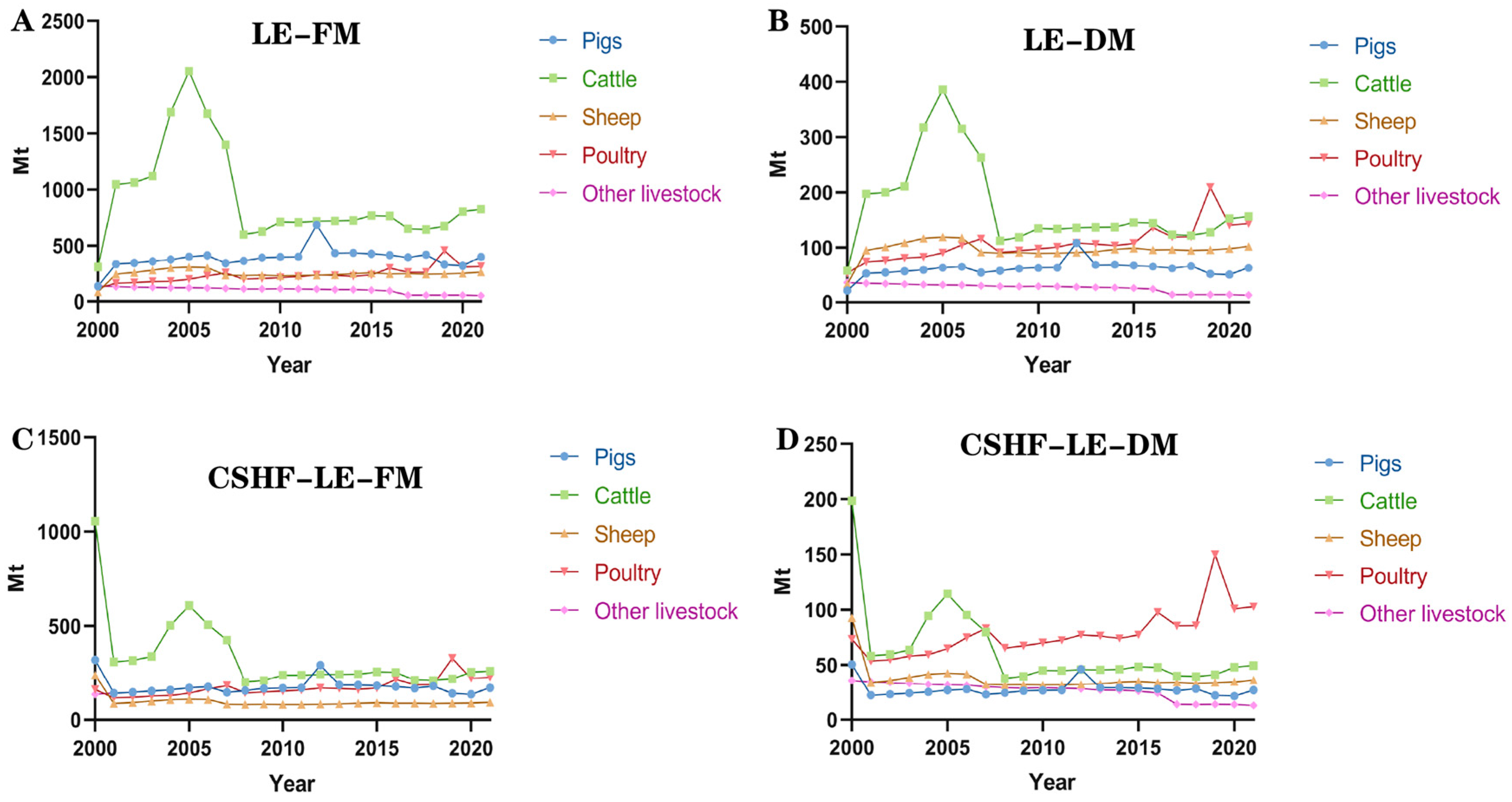
The estimation of LE emissions from China’s livestock industry indicates that the peak emissions occurred in 2005 at 3082.758 Mt/Year, which contradicts the findings of Peidong Z [40]. This discrepancy is suspected to be a result of data deviations, although there were no significant differences in the overall trend. The study identified four distinct stages of LE emissions in China, representing the historical trajectory of emissions in the country. The growth rate and efforts to address environmental issues varied across these stages. These findings highlight the need for continued efforts by China in the post-COVID-19 era to balance economic development with the sustainability of the livestock industry [41]. This suggests the importance of raising awareness and investing more in the management and mitigation of the environmental impact. Importantly, the COVID-19 pandemic did not have a significant impact on the growth of LE emissions, indicating that other factors play a more significant role. Additionally, the emissions from China’s commercial-scale husbandry feedlots (CSHF) were found to be consistent with normal LE emissions, suggesting that other types of livestock production systems also contribute to the growth and impact of LE emissions in China [42].

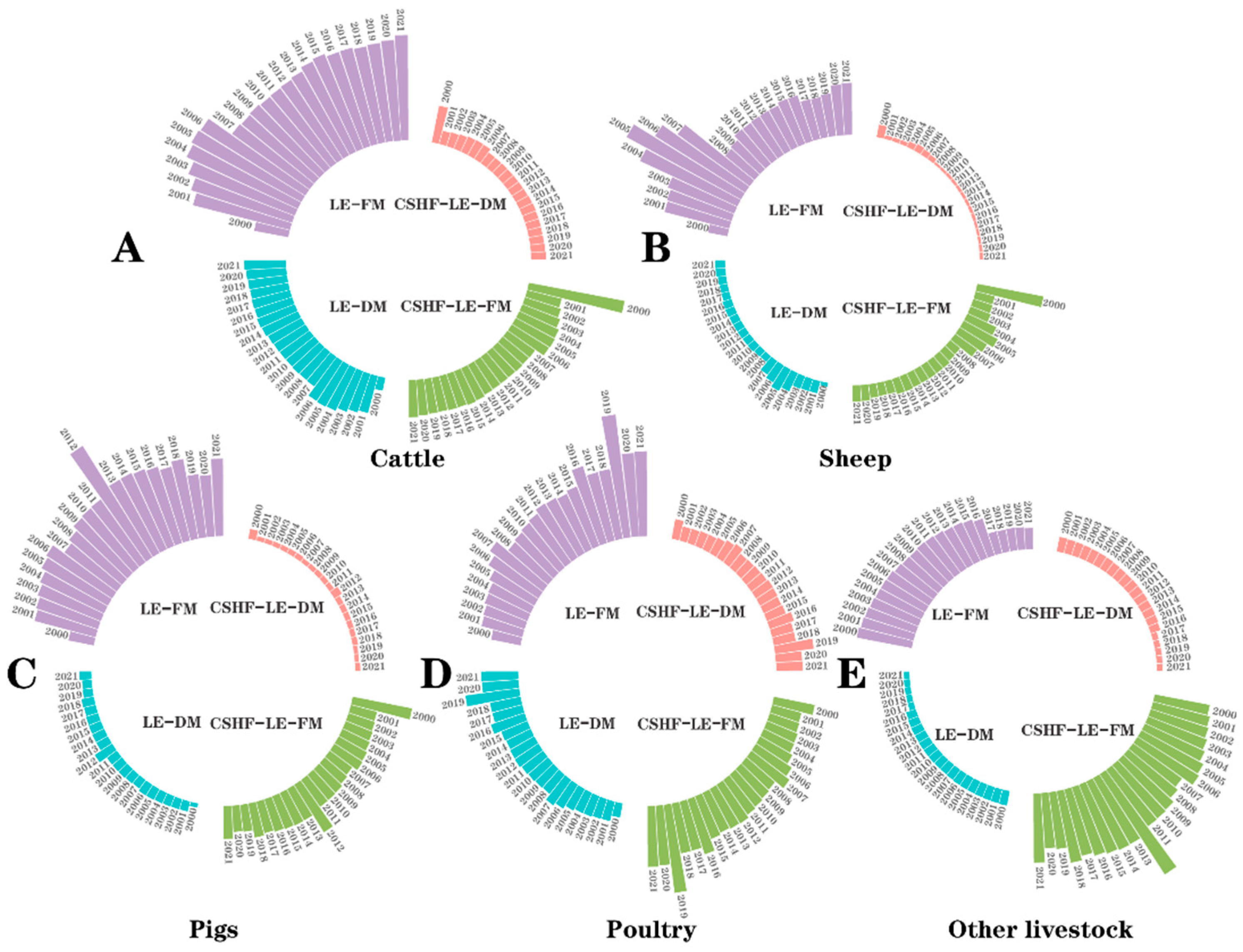
In terms of LE emissions from different livestock categories, cattle are considered the most significant contributors to LE-FM, followed by pigs. Poultry accounted for the largest proportion of LE-DM emissions. This pattern was confirmed in the study by Zhang T [43], which suggested that the specific moisture content in their manure might be responsible for it. The results also showed a significant upward trend in total LE emissions from poultry in recent years. These findings highlight the variation in the contributions and trends between different livestock species in terms of LE emissions. Considering the prominence of cattle and the increasing significance of poultry, China should implement targeted measures to mitigate their environmental impact by controlling LE emissions from these two livestock types [44].

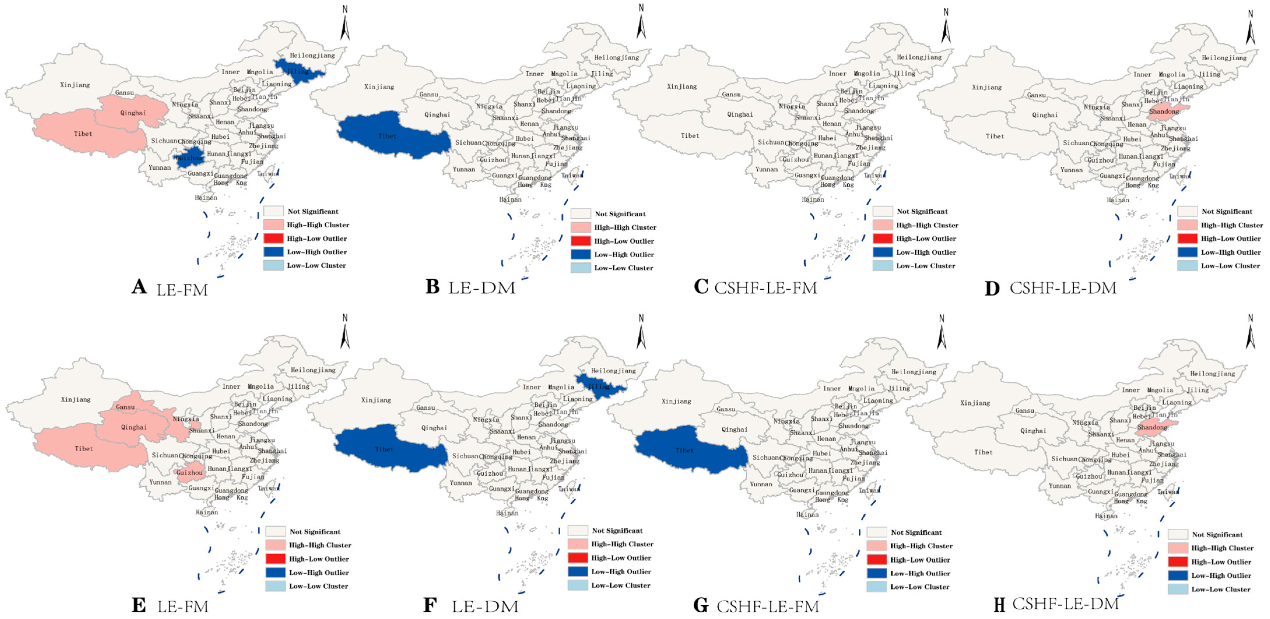
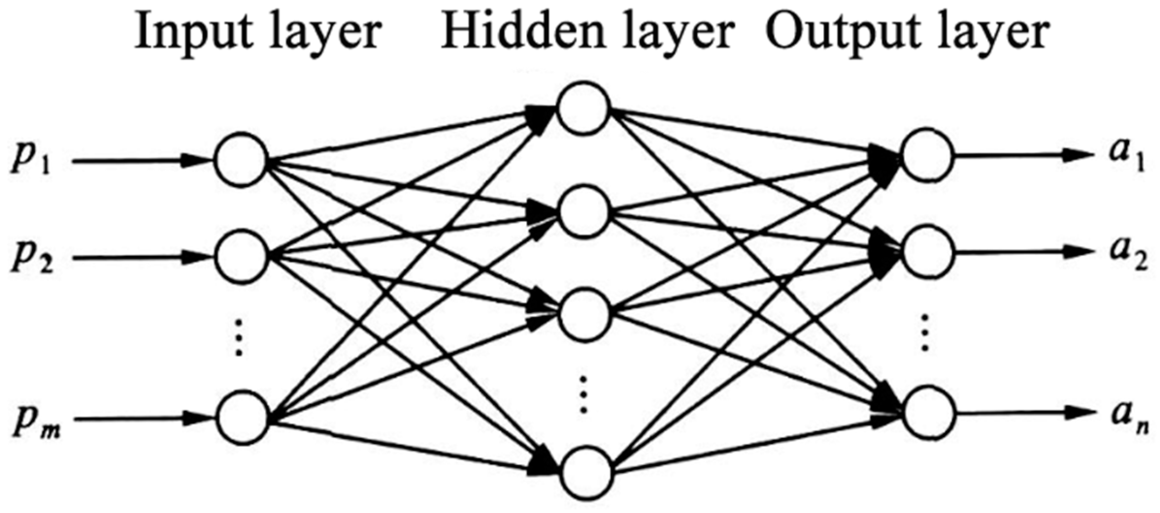
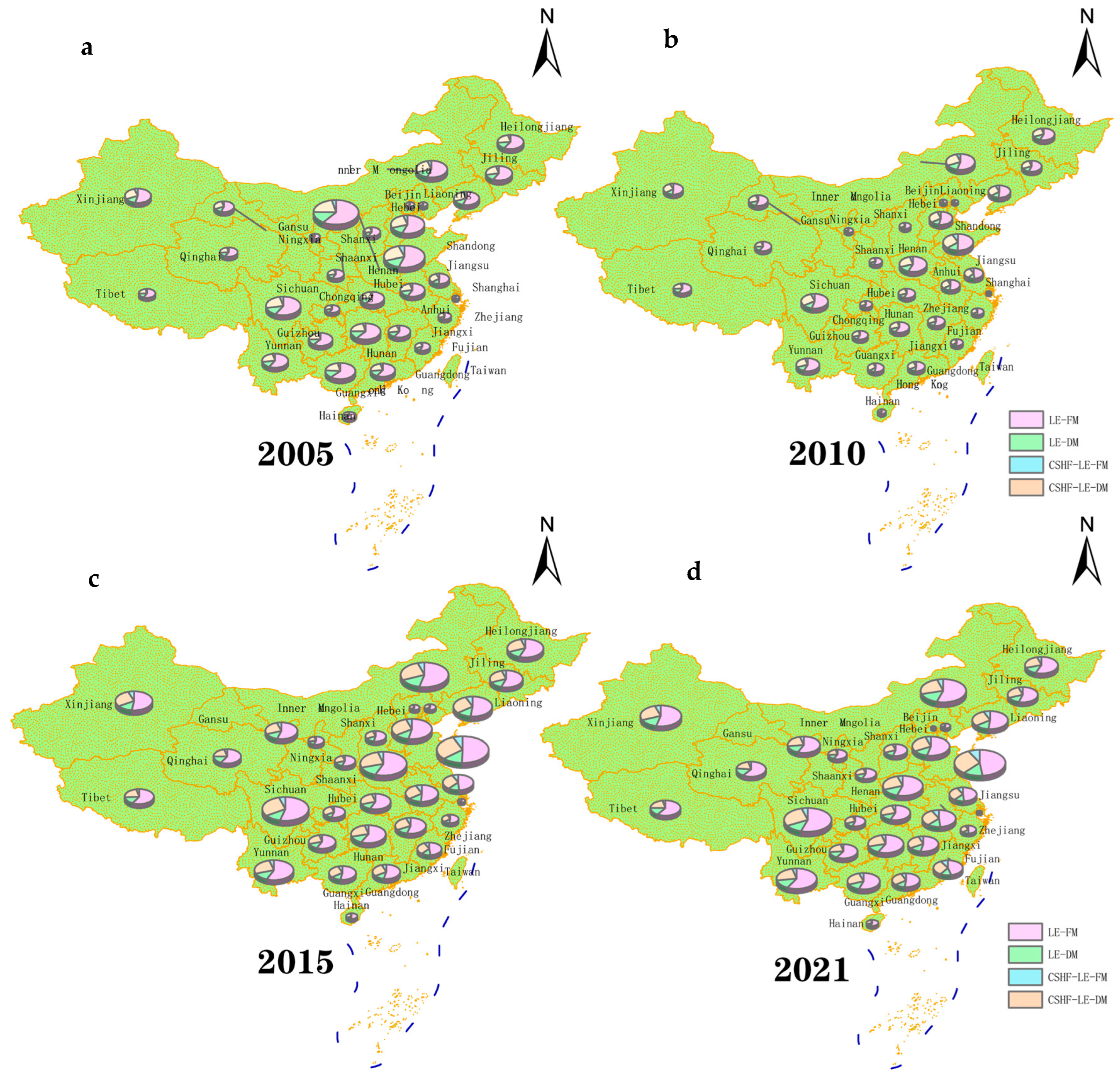
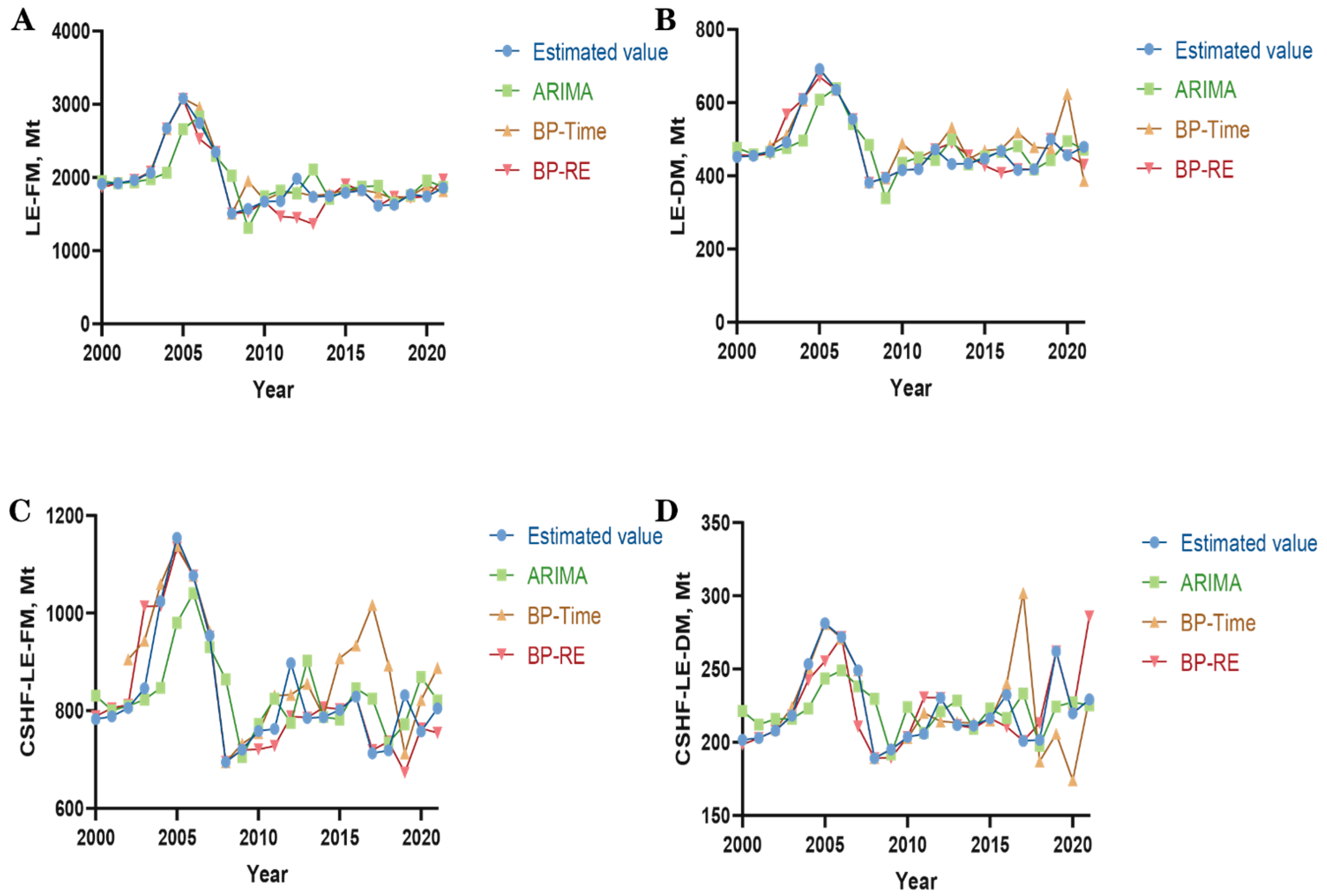
When investigating the spatial clustering characteristics of LE emissions across Chinese provinces, no significant spatial clustering patterns were observed, leading to the rejection of the second hypothesis proposed in this study. However, based on the results of global autocorrelation, there is a possibility that high–high clustering features may emerge in regions like Shandong and Sichuan in the future. This highlights the need for further investigation in future studies. To address this, China should implement rational planning and distribution strategies for LE emissions in spatial terms, which are essential for effectively assimilating and disposing of LE. One of the key innovations in this study was the prediction of LE emissions, which was crucial to verify the second hypothesis. Three prediction models were trained and fitted based on error rates, goodness of fit, and RMSE, and the BP-RE prediction model was adopted to forecast China’s LE emissions for the next ten years. By 2031, FM is projected to increase by 24.53% compared to 2021, while DM is expected to decrease by 28.06%. Under CSHF conditions, both FM and DM are predicted to rise by 11.16% and 2.05%, respectively. These findings indicate a change in livestock structure from 2021 to 2031, with a significant decline in free-range poultry possibly contributing to this phenomenon. Additionally, this change can be attributed to the increasing level of industrialization [45]. Therefore, China needs to innovate and improve the methods of handling LE-FM, while also increasing its utilization rate through techniques like composting and anaerobic digestion [46]. Furthermore, it is necessary to enhance the existing approaches to managing LE-DM, incorporating CSHF principles to improve FM and DM treatment under such conditions.

The limitations of this study are primarily related to the estimation of LE, which is based on formulas derived from previous research. This approach may introduce biases in the collection and calculation of data. Additionally, the analysis only considered one specific spatiotemporal model which may yield different results compared to other models. These limitations should be considered in future research.

5. Conclusions

According to the findings, the emissions of LE in China reached 3082.758 Mt/year for FM and 691.951 Mt/year for DM by 2005. The lowest emissions were recorded in 2008, with FM reaching 1508.665 Mt/year and DM reaching 380.970 Mt/year. In this study, the emissions of LE in China over the past 20 years have been estimated.

Judging from the results of global correlation analysis, there was no spatial correlation present among various provinces in China regarding LE emissions. However, the findings from local autocorrelation analysis indicated a strong likelihood of spatial positive correlation in China’s LE in the future, particularly in the regions like Shandong and Sichuan with high clustering. After thorough comparison and analysis of the prediction models, it was found out the BP-RE model performed best in predicting the emissions of LE in China. According to the projected outcome, the total amount of FM (fecal matter) in LE in China will reach 2313.949 billion tons by 2031, up by 24.53% compared to 2021. Conversely, DM (dung matter) emissions are projected to decrease by 28.06%, reaching 344.740 Mt by 2031. Under the conditions of CSHF (current stable housing facilities), the emissions of FM and DM are projected to reach 894.289 Mt and 233.913 Mt, respectively, up by 11.16% and 2.05%, respectively. These projections highlight the potential changes in the future demand of China for different types of livestock.

References

1. Vo, T.P.T.; Ngo, H.H.; Guo, W.; Turney, C.; Liu, Y.; Nguyen, D.D.; Bui, X.T.; Varjani, S. Influence of the COVID-19 pandemic on climate change summit negotiations from the climate governance perspective. Sci. Total Environ. 2023, 878, 162936. [Google Scholar] [CrossRef] [PubMed]
2. Yang, Y.; Luan, W.; Xue, Y. Sustainability and Environmental Inequality: Effects of Animal Husbandry Pollution in China. Sustainability 2019, 11, 4576. [Google Scholar] [CrossRef]
3. Li, F.; Cheng, S.K.; Yu, H.; Yang, D.W. Waste from livestock and poultry breeding and its potential assessment of biogas energy in rural China. J. Clean. Prod. 2016, 126, 451–460. [Google Scholar] [CrossRef]
4. Gu, P.; Shen, R.F.; Chen, Y.D. Diffusion pollution from livestock and poultry rearing in the Yangtze Delta, China. Environ. Sci. Pollut. Res. 2008, 15, 273–277. [Google Scholar] [CrossRef] [PubMed]
5. Wang, J.; Yang, H.; Chen, S.; Li, W.; Yu, J.; Hu, Z.; Zhuo, Y.; Huang, Q.; Liu, Z.; Zhou, L.; et al. Genome-wide association study reveals candidate genes for pollution excreta traits in pigs. Anim. Genet. 2023, 54, 553–557. [Google Scholar] [CrossRef]
6. Qian, Y.; Song, K.; Hu, T.; Ying, T. Environmental status of livestock and poultry sectors in China under current transformation stage. Sci. Total Environ. 2018, 622–623, 702–709. [Google Scholar] [CrossRef]
7. Wei, G.; Kong, X.; Wang, Y. Will Joining Cooperative Promote Farmers to Replace Chemical Fertilizers with Organic Fertilizers? Int. J. Environ. Res. Public Health 2022, 19, 16647. [Google Scholar] [CrossRef]
8. Khaliq, A.; Abbasi, M.K.; Hussain, T. Effects of integrated use of organic and inorganic nutrient sources with effective microorganisms (EM) on seed cotton yield in Pakistan. Bioresour. Technol. 2006, 97, 967–972. [Google Scholar] [CrossRef]
9. Fang, P.; Abler, D.; Lin, G.; Sher, A.; Quan, Q. Substituting Organic Fertilizer for Chemical Fertilizer: Evidence from Apple Growers in China. Land 2021, 10, 858. [Google Scholar] [CrossRef]
10. Hu, Y.; Li, D.; Wu, Y.; Liu, S.; Li, L.; Chen, W.; Wu, S.; Meng, Q.; Feng, H.; Siddique, K.H.M. Mitigating greenhouse gas emissions by replacing inorganic fertilizer with organic fertilizer in wheat-maize rotation systems in China. J. Environ. Manag. 2023, 344, 118494. [Google Scholar] [CrossRef]
11. Chen, Y.; Fu, X.; Liu, Y. Effect of Farmland Scale on Farmers’ Application Behavior with Organic Fertilizer. Int. J. Environ. Res. Public Health 2022, 19, 4967. [Google Scholar] [CrossRef]
12. Wei, Z.; Zhuang, M.; Hellegers, P. Towards circular nitrogen use in the agri-food system at village and county level in China. Agric. Syst. 2023, 209, 103683. [Google Scholar] [CrossRef]
13. Wu, C.; Huang, J.; Zhu, H.; Zhang, L.; Minasny, B.; Marchant, B.P.; McBratney, A.B. Spatial changes in soil chemical properties in an agricultural zone in southeastern China due to land consolidation. Soil Tillage Res. 2018, 187, 152–160. [Google Scholar] [CrossRef]
14. Mengqi, Z.; Shi, A.; Ajmal, M.; Ye, L.; Awais, M. Comprehensive review on agricultural waste utilization and high-temperature fermentation and composting. Biomass Convers. Biorefinery 2021, 13, 5445–5468. [Google Scholar] [CrossRef]
15. Cai, Y.; Tang, R.; Tian, L.; Chang, S.X. Environmental impacts of livestock excreta under increasing livestock production and management considerations: Implications for developing countries. Curr. Opin. Environ. Sci. Health 2021, 24, 100300. [Google Scholar] [CrossRef]
16. Ibekwe, A.M.; Bhattacharjee, A.S.; Phan, D.; Ashworth, D.; Schmidt, M.P.; Murinda, S.E.; Obayiuwana, A.; Murry, M.A.; Schwartz, G.; Lundquist, T.; et al. Potential reservoirs of antimicrobial resistance in livestock waste and treated wastewater that can be disseminated to agricultural land. Sci. Total Environ. 2023, 872, 162194. [Google Scholar] [CrossRef]
17. Shang, Z.; Wang, Y.; An, M.; Chen, X.; Kulyar, M.F.; Tan, Z.; Liu, S.; Li, K. The successional trajectory of bacterial and fungal communities in soil are fabricated by yaks’ excrement contamination in plateau, China. Front. Microbiol. 2022, 13, 1016852. [Google Scholar] [CrossRef]
18. Ngwabie, N.M.; Schade, G.W.; Custer, T.G.; Linke, S.; Hinz, T. Volatile organic compound emission and other trace gases from selected animal buildings. Landbauforsch. Volkenrode 2007, 57, 273. [Google Scholar]
19. Bannert, A.; Bogen, C.; Esperschütz, J.; Koubová, A.; Buegger, F.; Fischer, D.; Radl, V.; FuB, R.; Chronakova, A.; Elhottova, D. Anaerobic oxidation of methane in grassland soils used for cattle husbandry. Biogeosciences 2012, 9, 3891–3899. [Google Scholar] [CrossRef]
20. Xing, J.; Song, J.; Ren, J.; Yang, W.; Duan, H. Regional integrative benefits of converting livestock excrements to energy in China: An elaborative assessment from life cycle perspective. J. Clean. Prod. 2020, 275, 122470. [Google Scholar] [CrossRef]
21. Wang, Z.; Xing, A.; Shen, H. Effects of nitrogen addition on the combined global warming potential of three major soil greenhouse gases: A global meta-analysis. Environ. Pollut. 2023, 334, 121848. [Google Scholar] [CrossRef] [PubMed]
22. Song, H.X.; Peng, C.H.; Zhang, K.R.; Li, T.; Yang, M.X.; Liu, Q.Y.; Zhu, Q.A. Quantifying patterns, sources and uncertainty of nitrous oxide emissions from global grazing lands: Nitrogen forms are the determinant factors for estimation and mitigation. Glob. Planet. Change 2023, 223, 104080. [Google Scholar] [CrossRef]
23. Shim, S.; Reza, A.; Kim, S.; Ahmed, N.; Won, S.; Ra, C. Simultaneous Removal of Pollutants and Recovery of Nutrients from High-Strength Swine Wastewater Using a Novel Integrated Treatment Process. Animals 2020, 10, 835. [Google Scholar] [CrossRef]
24. Yamashita, T.; Hasegawa, T.; Hayashida, Y.; Ninomiya, K.; Shibata, S.; Ito, K.; Mizuguchi, H.; Yokoyama, H. Energy savings with a biochemical oxygen demand (BOD)- and pH-based intermittent aeration control system using a BOD biosensor for swine wastewater treatment. Biochem. Eng. J. 2022, 177, 108266. [Google Scholar] [CrossRef]
25. Frey, L.; Tanunchai, B.; Glaser, B. Antibiotics residues in pig slurry and manure and its environmental contamination potential. A meta-analysis. Agron. Sustain. Dev. 2022, 42, 31. [Google Scholar] [CrossRef]
26. Xue, Y.N.; Luan, W.X.; Wang, H.; Yang, Y.J. Environmental and economic benefits of carbon emission reduction in animal husbandry via the circular economy: Case study of pig farming in Liaoning, China. J. Clean. Prod. 2019, 238, 117968.1–117968.8. [Google Scholar] [CrossRef]
27. Du, X.; Zhang, Y.; Ma, Y.W.; Feng, S.X.; Zhang, Y.X.; Kou, H.J.; Sun, Y. The synergistic effect of chemical oxidation and microbial activity on improving volatile fatty acids (VFAs) production during the animal wastewater anaerobic digestion process treated with persulfate/biochar. Sci. Total Environ. 2023, 857, 159276. [Google Scholar] [CrossRef]
28. Li, D.; Yao, Y.; Sun, H.; Wang, Y.; Pu, J.; Calderón, R.; Alder, A.C.; Kannan, K. Artificial Sweeteners in Pig Feed: A Worldwide Survey and Case Study in Pig Farms in Tianjin, China. Environ. Sci. Technol. 2020, 54, 4059–4067. [Google Scholar] [CrossRef]
29. Bao, W.; Yang, Y.; Fu, T.; Xie, G.H. Estimation of livestock excrement and its biogas production potential in China. J. Clean. Prod. 2019, 229, 1158–1166. [Google Scholar] [CrossRef]
30. Zhang, Y.; Zhang, M.; Qin, Y.; Zhang, L.; Kang, D.; Wei, R.; Yang, C. Epidemiological analysis and risk prediction of scrub typhus from 2006 to 2021 in Sichuan, China. Front. Public Health 2023, 11, 1177578. [Google Scholar] [CrossRef]
31. Han, Z.; Huang, Q.; Huang, S.; Leng, G.; Bai, Q.; Liang, H.; Wang, L.; Zhao, J.; Fang, W. Spatial-temporal dynamics of agricultural drought in the Loess Plateau under a changing environment: Characteristics and potential influencing factors. Agric. Water Manag. 2021, 244, 106540. [Google Scholar] [CrossRef]
32. Haarr, M.L.; Falk-Andersson, J.; Fabres, J. Global marine litter research 2015–2020: Geographical and methodological trends. Sci. Total Environ. 2022, 820, 153162. [Google Scholar] [CrossRef] [PubMed]
33. Dai, M.; Huang, S.; Huang, Q.; Leng, G.; Guo, Y.; Wang, L.; Fang, W.; Li, P.; Zheng, X. Assessing agricultural drought risk and its dynamic evolution characteristics. Agric. Water Manag. 2020, 231, 106003. [Google Scholar] [CrossRef]
34. Kaur, J.; Parmar, K.S.; Singh, S. Autoregressive models in environmental forecasting time series: A theoretical and application review. Environ. Sci. Pollut. Res. 2023, 30, 19617–19641. [Google Scholar] [CrossRef]
35. Ghafouri-Fard, S.; Mohammad-Rahimi, H.; Motie, P.; Minabi, M.A.S.; Taheri, M.; Nateghinia, S. Application of machine learning in the prediction of COVID-19 daily new cases: A scoping review. Heliyon 2021, 7, e08143. [Google Scholar] [CrossRef] [PubMed]
36. Wang, W.; Liu, W.L.; Chen, H. Information granules-based BP Neural Network for Long-term Prediction of Time Series. IEEE Trans. Fuzzy Syst. 2020, 29, 2975–2987. [Google Scholar] [CrossRef]
37. Zhang, L.; Wang, F.; Xu, B.; Chi, W.; Wang, Q.; Sun, T. Prediction of stock prices based on LM-BP neural network and the estimation of overfitting point by RDCI. Neural Comput. Appl. 2017, 30, 1425–1444. [Google Scholar] [CrossRef]
38. Xu, L.; Quan, T.; Wang, J.; Gulliver, T.A.; Le, K.N. GR and BP neural network-based performance prediction of dual-antenna mobile communication networks. Comput. Netw. 2020, 172, 107172. [Google Scholar] [CrossRef]
39. Hong-Wei, T.; Jian-Yuan, C.; Shi-Dong, W. The Effective Application of BP Neural Networks Prediction Model for Gas Content in Binchang Mining. In Proceedings of the International Conference on Computational Intelligence and Software Engineerin, Wuhan, China, 11–13 December 2009. [Google Scholar] [CrossRef]
40. Zhang, P.; Yang, Y.; Tian, Y.; Yang, X.; Zhang, Y.; Zheng, Y.; Wang, L. Bioenergy industries development in China: Dilemma and solution. Renew. Sustain. Energy Rev. 2009, 13, 2571–2579. [Google Scholar] [CrossRef]
41. Hao, G.; Zhu, H.; Cui, Y. Measurement and Influencing Factors of Carbon Emissions of China’s Livestock Husbandry in the Post-COVID-19 Era—Based on the Supply-Side Perspective. Sustainability 2023, 15, 913. [Google Scholar] [CrossRef]
42. Abu Hatab, A.; Krautscheid, L.; Boqvist, S. COVID-19, Livestock Systems and Food Security in Developing Countries: A Systematic Review of an Emerging Literature. Pathogens 2021, 10, 586. [Google Scholar] [CrossRef]
43. Zhang, T.; Bu, M.D.; Geng, W. Pollution status and biogas-producing potential of livestock and poultry excrements in China. Chin. J. Ecol. 2012, 31, 1241. [Google Scholar]
44. Zhou, L.; Zhang, J.; Zhang, X.; Zhang, J. A Leading Role of Water Resources and Animal Husbandry in Environmental Sustainability: A Case Study of China. Environ. Sci. Pollut. Res. 2023, 30, 72146–72159. [Google Scholar] [CrossRef] [PubMed]
45. Zhan, N.; Liu, W.; Ye, T.; Li, H.; Chen, S.; Ma, H. High-resolution livestock seasonal distribution data on the Qinghai-Tibet Plateau in 2020. Sci. Data 2023, 10, 142. [Google Scholar] [CrossRef] [PubMed]
46. Liu, C.; Liao, W.; Xu, Y.; Wu, D.; Gao, Z.; Xie, J. Characterizing NH3 emissions from a sheep feedlot and a manure composting facility in North China with the inverse dispersion technique. Agric. For. Meteorol. 2023, 339, 109580. [Google Scholar] [CrossRef]
Figure 1. BP neural network structure diagram, mainly consisting of three parts, distributed as input layer, hidden layer, and output layer.
Agriculture 13 02143 g001
Figure 2. The differences in livestock excreta (LE) emissions among various types of livestock can be observed. (A) The fresh weight is displayed. (B) The dry weight is displayed. (C) It illustrates the emissions of fresh weight under intensive agricultural conditions. (D) The emissions of dry weight under the same conditions are displayed. The Y-axis in each graph represents emission quantity measured in Mt (megatons), while the X-axis represents the timeline from 2000 to 2021. The blue line represents pigs, the green line represents cattle, the yellow line represents sheep, the red line represents birds, and the purple line denotes other animals.
Agriculture 13 02143 g002
Figure 3. The changes in livestock excreta (LE) emissions for different types of animals are demonstrated. (A) illustrates the variations in fresh weight and dry weight emissions of cattle over time, along with the histograms depicting fresh weight and dry weight emissions under intensive farming conditions. (B) displays the histogram showcasing the changes in sheep emissions over time. (C) represents the variations in pig emissions. (D) depicts the histogram illustrating the fluctuations in poultry emissions over time. Lastly, (E) demonstrates the histograms displaying the changes in emissions from other animals over time.
Agriculture 13 02143 g003
Figure 4. (a) Distribution trend of livestock emissions in China in 2005. (b) Distribution trend of livestock emissions in China in 2010. (c) Distribution trend of livestock emissions in China in 2015. (d) Distribution trend of livestock emissions in China in 2021. The emissions of different regions are represented by pie charts, where a larger diameter indicates higher emission levels. The various colors represent different weights: pink represents fresh weight and green represents dry weight, while blue and yellow represent fresh weight and dry weight under intensive farming conditions.
Agriculture 13 02143 g004
Figure 5. The figure illustrates the fitting line graphs of predicted values and actual values from different forecasting models. Panel (A) represents the fresh weight emissions and panel (B) represents the dry weight emissions, while panels (C,D) depict the emissions of fresh weight and dry weight under intensive farming conditions. The Y-axis represents the emission quantity in Mt, and the X-axis represents the years from 2000 to 2021. The blue line represents the estimated LE emission values, the green line represents the results of ARIMA time series forecasting, the yellow line represents the results of BP neural network time series prediction model, and the red line represents the results of BP neural network regression prediction model.
Agriculture 13 02143 g005