Smart Temperature and Humidity Control in Pig House by Improved Three-Way K-Means

Abstract

Efficiently managing temperature and humidity in a pig house is crucial for enhancing animal welfare. This research endeavors to develop an intelligent temperature and humidity control system grounded in a three-way decision and clustering algorithm. To establish and validate the effectiveness of this intelligent system, experiments were conducted to compare its performance against a naturally ventilated pig house without any control system. Additionally, comparisons were made with a threshold-based control system to evaluate the duration of temperature anomalies. The experimental findings demonstrate a substantial improvement in temperature regulation within the experimental pig house. Over a 24 h period, the minimum temperature increased by 4 °C, while the maximum temperature decreased by 8 °C, approaching the desired range. Moreover, the average air humidity decreased from 73.4% to 68.2%. In summary, this study presents a precision-driven intelligent control strategy for optimizing temperature and humidity management in pig housing facilities.

1. Introduction

Pigs are thermoregulatory animals that maintain a dynamic equilibrium between heat production and heat dissipation through physiological mechanisms. Maintaining appropriate temperature and humidity levels is paramount for ensuring the normal growth and development of pigs [1,2,3]. When the ambient temperature exceeds the thermoneutral zone, pigs adjust their heat production and energy intake to mitigate the effects of heat stress [4,5,6]. Elevated ambient temperatures can significantly increase the incidence and mortality rates among pigs, compromise animal welfare, and result in substantial economic losses [7,8,9,10]. Prolonged exposure to high temperatures can suppress the pig’s immune response, disrupt thermal equilibrium, and lead to severe conditions such as heat stroke, coma, and even fatality [11,12]. Conversely, continuous exposure to low temperatures can predispose pigs to respiratory and digestive system ailments as well as conditions like rheumatism and arthritis [13,14,15]. In modern pig housing facilities, frequently used for intensive livestock production, various methods including natural or mechanical ventilation and the use of dehumidifiers are employed to regulate indoor conditions [16,17,18]. It is imperative in livestock buildings to establish and maintain an optimal and comfortable environment, as this directly impacts both production efficiency and animal welfare [19,20,21,22]. Environmental temperature and air humidity rank as the most influential climatic factors affecting pig production, with temperature fluctuations exerting a substantial influence on pigs’ well-being. Excessive heat can induce heat stress, which disrupts feed intake, digestion, and nutrient absorption, ultimately resulting in decreased productivity [23,24,25,26]. Therefore, the implementation of an intelligent temperature and humidity control system is indispensable in livestock buildings to optimize production outcomes.

As the indoor environment of livestock housing directly affects the growth of livestock, a temperature and humidity control system is needed to ensure productivity. Ulpiani et al. [27] devised three distinct logic switches for regulating heating systems within livestock housing. Meanwhile, Xie et al. [28] conducted a comprehensive study on the design and control strategies of a closed-pig-house environmental regulation system, which not only fosters a comfortable environment for pig growth but also provides valuable insights for further advancements in livestock environmental control. In a related effort, Gao et al. [29] developed a microclimate simulation model tailored for broiler houses, leveraging the structural characteristics of these facilities and parameters specific to chick growth environments. This model incorporates fuzzy logic inference techniques to generate diverse control strategies considering various environmental factors. On the other hand, Xie et al. [30] introduced a model for predicting indoor temperatures by integrating the energy balance equation (EBE) and adaptive neuro-fuzzy inference system (ANFIS). They employed weather conditions and indoor environmental data from pig houses as input variables, enabling precise temperature forecasts. Li et al. [31] contributed to the field by discussing key technologies and facilities for large-scale chicken environmental regulation in China. Additionally, they proposed models advocating intelligent farming practices and welfare-oriented farming. Dmitry et al. [32] proposed an innovative thermoelectric air dehumidification unit designed to control the microclimate in cattle-breeding farms using Peltier elements. This system activates thermoelectric elements, fans, and a circulation pump when the indoor air’s relative humidity exceeds the predefined upper limit. The unit effectively extracts humid air, cools and dries it through an air heat exchanger, and utilizes ozone for partial air cleaning and disinfection before reintroducing the conditioned air into the premises. This process steadily reduces indoor air humidity until it reaches the preset level, at which point the dehumidification unit ceases operation. Furthermore, Du et al. [33] developed an intelligent monitoring system for chicken houses. This system continuously monitors real-time temperature fluctuations within the chicken house. When the indoor temperature surpasses the predefined threshold, the system dynamically adjusts the output power of the temperature control device based on the temperature difference between the indoor environment and the set threshold. Higher differences trigger higher output power levels, ensuring the indoor temperature returns to the desired normal range. Currently, prevalent temperature and humidity control systems in livestock buildings rely on single-variable control mechanisms using threshold settings due to their simplicity and cost-effectiveness. However, these traditional methods, while effective at restoring indoor temperature and humidity to desired levels, address only one variable at a time and are prone to temperature and humidity anomalies. Consequently, these control approaches may not consistently maintain temperature and humidity within the appropriate ranges.

This paper proposed an intelligent control system for temperature and humidity in pig houses based on a three-way decision and clustering algorithm. Our system provides pigs with a suitable breeding environment by adjusting the temperature and humidity in the pigsty. Compared to threshold-based control systems, our system has fewer abnormal temperature occurrences. This paper makes the following key contributions:

(1)

Proposed an improved three-way k-means algorithm TWKS, optimizing the selection of initial cluster centers and enhancing the performance of clustering results.

(2)

Using k-means, historical weather data are clustered according to a control strategy. The newly collected weather data are then classified using the K-nearest neighbor algorithm.

(3)

Compared to traditional threshold-based control systems, the system proposed in this paper is more intelligent as it eliminates the need for threshold settings and reduces temperature anomaly duration.

(4)

The intelligent control system proposed in this paper is experimented within pigsties, but it is also applicable to temperature and humidity control in other livestock buildings such as chicken coops, cowsheds, greenhouses, etc.

2. Materials and Methods

Pigs are thermostatic animals characterized by their thick subcutaneous fat and relatively undeveloped sweat glands. They exhibit a high sensitivity to environmental factors such as air temperature and relative humidity. Consequently, maintaining optimal temperature and humidity levels within the pig housing facility is of paramount importance. The primary focus of this study centers on the development of an intelligent control system designed to regulate temperature and humidity within the pig housing environment. This system leverages the utility of three-way k-means clustering models to effectively allocate control strategies through a comprehensive analysis of multidimensional meteorological data. The model takes into consideration a range of input variables, including indoor air temperature ($T_i$), outdoor air temperature ($T_o$), indoor relative humidity ($H_i$), outdoor relative humidity ($H_o$), wind speed ($W_s$), wind direction ($W_d$), surface temperature ($T_s$), and surface pressure ($P_s$), with the control scheme serving as the output variable (as depicted in Figure 1).

2.1. Temperature and Humidity Control Strategy

2.1.1. Sample Stability

Li et al. [34] introduced the sample stability in the clustering ensemble and proposed a clustering ensemble based on the sample stability. This subsection is reviewed for the sample stability.

Suppose $X=\{x_1,x_2,\dots ,x_n\}$ is a dataset with n samples and $Q=\{q_1,q_2,\dots ,q_L\}$ is the set of clustering results after L clustering using the same clustering algorithm with different parameters or different clustering algorithms. Define $P_{ij}$ to denote the frequency with which samples $x_i$ and $x_j$ are assigned to the same cluster:

$$P_{ij}=\frac{1}{L}\sum _{i=1}^{L}H(q_l\left(x_i\right),q_l\left(x_j\right))$$

(1)

where

$$H(q_l\left(x_i\right),q_l\left(x_j\right))=\left\{\begin{array}{cc}1& q_l\left(x_i\right)=q_l\left(x_j\right)\\ 0& q_l\left(x_i\right)\ne q_l\left(x_j\right)\end{array}\right..$$

(2)

If the sample is assigned to the same cluster in the l-th cluster, then the value of $H(q_l\left(x_i\right),q_l\left(x_j\right))$ is 1; otherwise, the value is 0.

After calculating the co-occurrence frequency between all samples, a relationship matrix P will be generated, which is used to represent the relationships between samples. When $P_{ij}$ is equal to 1, it means that samples $x_i$ and $x_j$ are assigned to the same cluster in multiple clusters, and the relationships between the two samples are stable. When $P_{ij}$ is equal to 0, it means that samples $x_i$ and $x_j$ are assigned to the different clusters in multiple clusters, and the relationships between the two samples are also stable. When $P_{ij}$ is greater than 0 but less than 1, it means that samples $x_i$ and $x_j$ are sometimes assigned to the same cluster and sometimes assigned to different cluster in multiple clusters; thus, the relationship between the two samples is unstable.

Based on the analysis above, the stable relationships between two samples can be identified in two ways: (1) if most clustering results assign them to the same cluster or (2) if most clustering results assign them to different clusters. Therefore, relying solely on co-occurrence frequency is insufficient to distinguish the relationship between samples. To address this, a stability function was proposed as an evaluation indicator for differentiating samples [34]. This function calculates the stability by averaging the certainty of frequency between one sample and another. The formula for calculating the stability of a sample is as follows:

$$s\left(x_i\right)=\frac{1}{n}\sum _{j=1}^{n}f\left(P_{ij}\right)$$

(3)

where $x_i$ denotes the i-th sample of the dataset, n denotes the number of the dataset, $f\left(P_{ij}\right)$ denotes the mapping function, and the calculation function is as follows:

$$f\left(P_{ij}\right)=\left\{\begin{array}{cc}|\frac{P_{ij}-t_0}{t_0}|& P_{ij}<t_0\\ |\frac{P_{ij}-t_0}{1-t_0}|& P_{ij}\ge t_0\end{array}\right..$$

(4)

where $t_0$ is the threshold calculated using the maximum variance threshold method [35], and the calculation process is as follows.

Assume the relationship matrix composed of co-occurrence frequency $P_{ij}$ is $P=p_1,p_2,\dots ,p_w$. We divide P into two parts $P_0$ and $P_1$, using a threshold $t_0$∈ (0,1).

$$P_0=\{p_i,p_i<t_0,1\le i\le w\}$$

(5)

$$P_1=\{p_i,p_i\ge t_0,1\le i\le w\}$$

(6)

Evaluate the performance of each threshold by calculating the inter-class variance, and select the most suitable threshold. The formula for calculating the inter-class variance ${\sigma }_t$ is as follows:

$${\sigma }_t={\omega }_0{({\mu }_0-\mu )}^2+{\omega }_1{({\mu }_1-\mu )}^2$$

(7)

$${\omega }_0=\frac{|P_0|}{\left|P\right|},{\omega }_1=\frac{|P_1|}{\left|P\right|}$$

(8)

$$\mu =\frac{{\displaystyle \sum _{p_i\in P}}{p}_i}{\left|P\right|},{\mu }_0=\frac{{\displaystyle \sum _{p_i\in P_0}}{p}_i}{|P_0|},{\mu }_1=\frac{{\displaystyle \sum _{p_i\in P_1}}{p}_i}{|P_1|}$$

(9)

By maximizing the inter-class variance ${\sigma }_t$, the optimal threshold $t_0$ is obtained.

2.1.2. Dividing the Dataset Based on Sample Stability

Given a dataset $X=\{x_1,x_2,\dots ,x_n\}$ containing n samples with a clustering number of k, the clustering result set $Q=\{q_1,q_2,\dots ,q_L\}$ obtained after multiple clusters is divided into a kernel dataset $K\left(X\right)$ and an outer dataset $R\left(X\right)$ by the following steps:

(1)

Calculate the co-occurrence frequency by formula (1) and then construct a relationship matrix P;

(2)

Calculate the threshold $t_0$ of the relationship matrix using formula (7) with P as input;

(3)

Calculate the stability $s\left(x_i\right)$ of each sample in the dataset using formula (3) to obtain the stability set S;

(4)

Calculate the stability threshold $s_0$ using formula (7) with S as input;

(5)

Kernel dataset $K\left(X\right)=\{x_i\in X|s\left(x_i\right)>s_0\}$

Outer dataset $R\left(X\right)=\{x_i\in X|s\left(x_i\right)\le s_0\}$.

2.1.3. Three-Way k-Means Algorithm for Optimizing Initial Cluster Centers

The central concept of the algorithm presented in this paper, which pertains to the selection of initial cluster centers, aims to ensure their placement within the dataset rather than at its periphery. Additionally, it strives to maintain a certain minimum separation between each pair of cluster centers. This approach serves a dual purpose: firstly, it reduces the frequency of updates to the cluster centers, and secondly, it enhances the overall performance of the clustering results. When visualizing the dataset as a spatial circle, the initial cluster centers are strategically chosen within a predefined distance from the circle’s center, forming a circular region. This selection strategy endeavors to distribute the initial cluster centers across different clusters as evenly as possible.

For the implementation of the algorithms in this study, Python 3.8 was employed as the programming language of choice. The subsequent section will provide a comprehensive elucidation of the steps involved in the algorithm, offering a detailed walkthrough of Algorithm 1.

In step 1, use the sample stability to divide the dataset into a kernel dataset and outer dataset.

In step 2, for each sample x in the kernel dataset $K\left(X\right)$, perform the following steps.

In step 3, calculate the median value of each dimension attribute of the samples in the kernel dataset, and use it as the first initial cluster center.

In step 4, calculate the maximum Euclidean distance, denoted as d, between the samples within the kernel dataset and the first initial cluster center.

In steps 5–8, find all the samples within the kernel dataset that have Euclidean distances from the first initial cluster center greater than 0.3d and less than 0.7d. Sort them in descending order based on their stability. Select the sample with the highest stability from the samples as the second initial cluster center.

In step 9, choose the remaining $k-$2 initial cluster centers from the sorted samples, ensuring that the Euclidean distance between any two initial cluster centers is not less than 0.3d.

In steps 11–17, after obtaining k initial cluster centers, calculate the Euclidean distance between the samples in the kernel dataset and the initial cluster centers. Assign the samples to the core domains of the cluster that are closest to them in terms of distance. Calculate the Euclidean distance between the samples in the outer dataset and the initial cluster centers. Assign the samples to the boundary domains of the cluster that is closest to them in terms of distance. Update the cluster centers by calculating the average value of each dimension attribute of all samples within each cluster as the new cluster center. Compare the k new cluster centers with the original cluster centers. If the cluster centers no longer change or reach the maximum number of iterations, stop the process.

In step 18, output the three-way k-means result.

Algorithm 1 Improved three-way k-means

Input:  dataset X, the number of cluster k Output:  three-way k-means C 1: Divide the dataset X into a kernel dataset $K\left(X\right)$ and outer dataset $R\left(X\right)$ by sample stability; 2: for each sample x in $K\left(X\right)$ do 3:  $m_1^{\prime }$← calculate the median value of each dimension attribute of samples; 4:  d← calculate the maximum Euclidean distance between samples and $m_1^{\prime }$; 5:  if 0.3d< distance between samples and $m_1^{\prime }$< 0.7d then 6:   Sort the samples according to their stability; 7:  end if 8:  $m_2^{\prime }$← select the sample with the highest stability among sorted samples; 9:  Select the remaining k-2 initial cluster centers from the sorted samples, ensuring that the Euclidean distance between any two initial cluster centers is not less than 0.3d; 10: end for 11: repeat 12:  Calculate the Euclidean distance between samples ∈$K\left(X\right)$ and cluster centers; 13:  Assign the samples to the core region of the cluster that is closest to their respective cluster centers; 14:  Calculated the Euclidean distance between samples ∈$R\left(X\right)$ and cluster centers; 15:  Assign the samples to the boundary region of the cluster that is closest to their respective cluster centers; 16:  Update the cluster centers ← calculate the mean value of samples in the cluster as the new cluster center; 17: until the cluster centers no longer change or reach the maximum allowed number of iterations. 18: Output the three-way k-means result.

2.1.4. Temperature and Humidity Optimization Control Algorithm

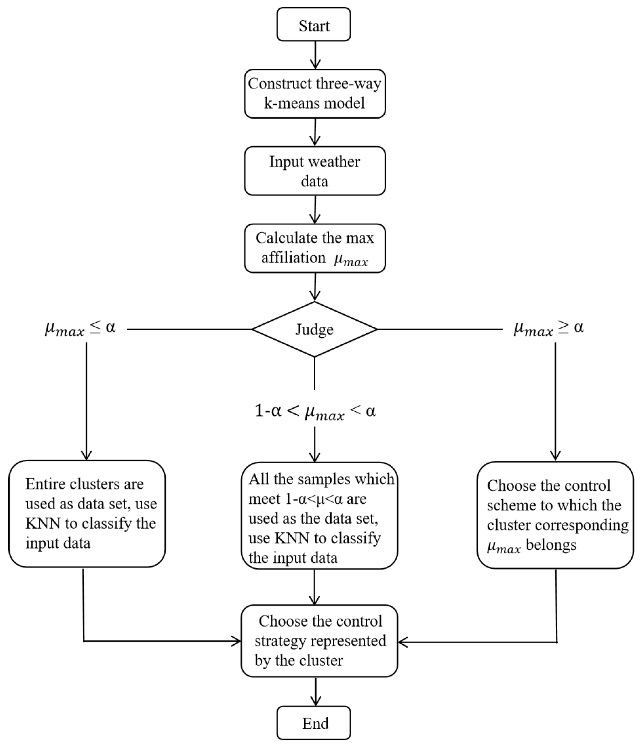
This article presents an intelligent control system for temperature and humidity in pig houses, which is based on the three-way k-means clustering model. The system utilizes historical data as a training set to construct the three-way k-means clustering model, where each cluster represents a specific temperature and humidity control scheme. Multiple-dimensional weather data are then inputted into the model to analyze the structural characteristics of the input data and match them with the appropriate clusters. By considering various attributes of the weather data, including inside air temperature, outside air temperature, inside relative humidity, outside relative humidity, wind speed, wind direction, surface temperature, and surface pressure, the system determines the most suitable temperature and humidity control scheme for the pig house. This, in turn, activates or deactivates the corresponding devices to maintain the temperature and humidity within an optimal range. Figure 2 illustrates the adjustment process based on the three-way k-means model, while Figure 3 depicts the block diagram of the temperature and humidity control system.

• Determine input–output variables of the model.
• Construct three-way clustering on history data, with the number of clusters being the number of temperature and humidity control schemes. After clustering, each cluster represents a temperature and humidity control scheme.
• Using sensors to monitor weather data, such as inside temperature, outside temperature, inside humidity, outside humidity, wind speed, wind direction, surface temperature, and surface pressure, these data are used as input to cluster the data based on the clustering centers of the clustering model. Set a threshold $\alpha$, calculate the affiliation of the input data with the center of each cluster, and select the maximum affiliation to be recorded ${\mu }_{max}$.
• If ${\mu }_{max}$ is greater than or equal to $\alpha$, then the control state to which the cluster corresponding to ${\mu }_{max}$ belongs is chosen.
• If ${\mu }_{max}$ is less than $\alpha$ and greater than or equal to 1$-\alpha$, then these input data may belong to the boundary domains of multiple clusters, and all the samples of the boundary domains of clusters whose affiliation with these input data is less than $\alpha$ and greater than 1$-\alpha$ are used as the classification dataset, and the k-nearest neighbor algorithm is used to classify the input data in terms of the control state.
• If ${\mu }_{max}$ is less than 1$-\alpha$, then the data of entire clusters are used as a categorized dataset, and the k-nearest neighbor algorithm is used to categorize the input data in terms of control state.
• Based on the assigned cluster, determine whether temperature and humidity control is required. If not, the program ends; if yes, start or stop the corresponding devices based on the control strategy associated with the cluster.
• Using sensors to monitor weather data, repeat the above process.

2.2. Data Preprocessing

Due to sensor failure, damage, and other factors, the weather data measured from the sensors may have outliers, which affects the accuracy of the model. Therefore, we preprocessed the dataset before training the k-means model, including abnormal data handling and data normalization.

2.2.1. Abnormal Data Handling

The abnormal data refer to outliers with unreasonable values in the dataset, which has the characteristic that the proportion in the whole dataset is usually small and deviates from the whole. Commonly used abnormal data detection algorithms include clustering-based outlier detection [36,37,38], density-based outlier detection [39,40], and so on. In this paper, we choose the isolated forest algorithm [41], which divides the dataset by constructing a binary tree, expresses the degree of alienation from the data subject according to the depth of the data samples in the binary tree, and finally divides the anomalous data by the anomaly score.

After detecting the abnormal data, it is necessary to correct the abnormal data. Calculate the k normal samples that are closest to the abnormal sample and use the average of the data from the k normal samples as the repair value for the abnormal data.

2.2.2. Data Normalization

Different attributes in the dataset have different dimensions and dimension units, which will affect the validity of the results of data analysis. Therefore, in order to eliminate the impact of dimensionality between attributes, data standardization is necessary, and the processed data range from [0,1], with each attribute in the same order of magnitude, which facilitates comprehensive evaluation. In addition, data standardization can also improve the speed and accuracy of data processing.

This paper adopts min − max standardization, and the calculation formula is shown as follows:

$$x^{\prime }=\frac{x-min}{max-min}$$

(10)

where $x^{\prime }$ represents the data attribute after normalization, x represents the original data attribute, $min$ represents the minimum value of the data attribute and $max$ represents the maximum value of the data attribute.

2.3. Experimental Setup

2.3.1. Description of the Experimental Pig House

The experimental pig house is located in Fenyang City, Shanxi Province, China (111°26′ E–112°00′ E, 37°08′ N–37°29′ N). The dimensions of the pig house are 21 m × 8.8 m × 3.55 m, with 240 mm thick brick walls plastered both inside and outside. The wall materials and thickness are the same on all sides, and the windows are single-layer plastic steel windows. There are 7 windows of size 1.5 m × 1.5 m on the south longitudinal wall and the north longitudinal wall. The lower edge of the windows is 0.7 m above the ground inside the house. The layout inside the pig house consists of double-row pig pens and a single-row aisle with a width of 1.37 m for the aisle. There are 14 pig pens inside the pig house, each measuring 2.90 m × 3.71 m with a height of 1 m. The solid floor width inside the pens is 2.6 m, and the slatted floor width is 4.8 m. There are 4 manure pits under each slatted floor, with a depth of 0.7 m. The manure is cleared by plug-type flushing. Each pig house has one door measuring 2.5 m (height) × 1.23 m (width). The experimental house is designed to raise 158 fattening pigs, aged 80 to 100 days. (the total area of the pig pens is 148.55 m${}^2$, and each fattening pig occupies a floor area of 0.8–1.2 m${}^2$). The breeds include Large White and Yorkshire, with an average body weight of 100–110 kg per pig. The roof is made of double-sloped color steel sandwich panels (100 mm thick), and the pig house has a 2.65 m high single-layer color steel ceiling.

2.3.2. Description of the Experimental Equipment

The HC2S3 sensors are installed at a height of 1.5 m above the roof of the pig house to measure environmental parameters. Surface temperature is measured by a thermometer 2 m from the pig house and 0.3 m from the floor. Within each enclosure of the pig house, an HC2S3 sensor is installed at a height of 1.5 m above the internal floor to measure internal parameters such as temperature and relative humidity. They are protected and designed with a 41003-5 radiation shield and equipped with a polyethylene filter to prevent dust and particles from entering, ensuring the reliability of sensor measurements. The temperature measurement range is −40 to 100 °C, with an accuracy of 0.1 °C and an error of ±0.1 °C. The humidity measurement range is 0 to 100%, with an accuracy of 0.1% and an error of ±0.8%. The wind velocity at 3 m above the ground is measured by an anemometer, with a sensitivity of 0.01 ms${}^{-1}$.

2.3.3. Description of the Experimental Site Setting

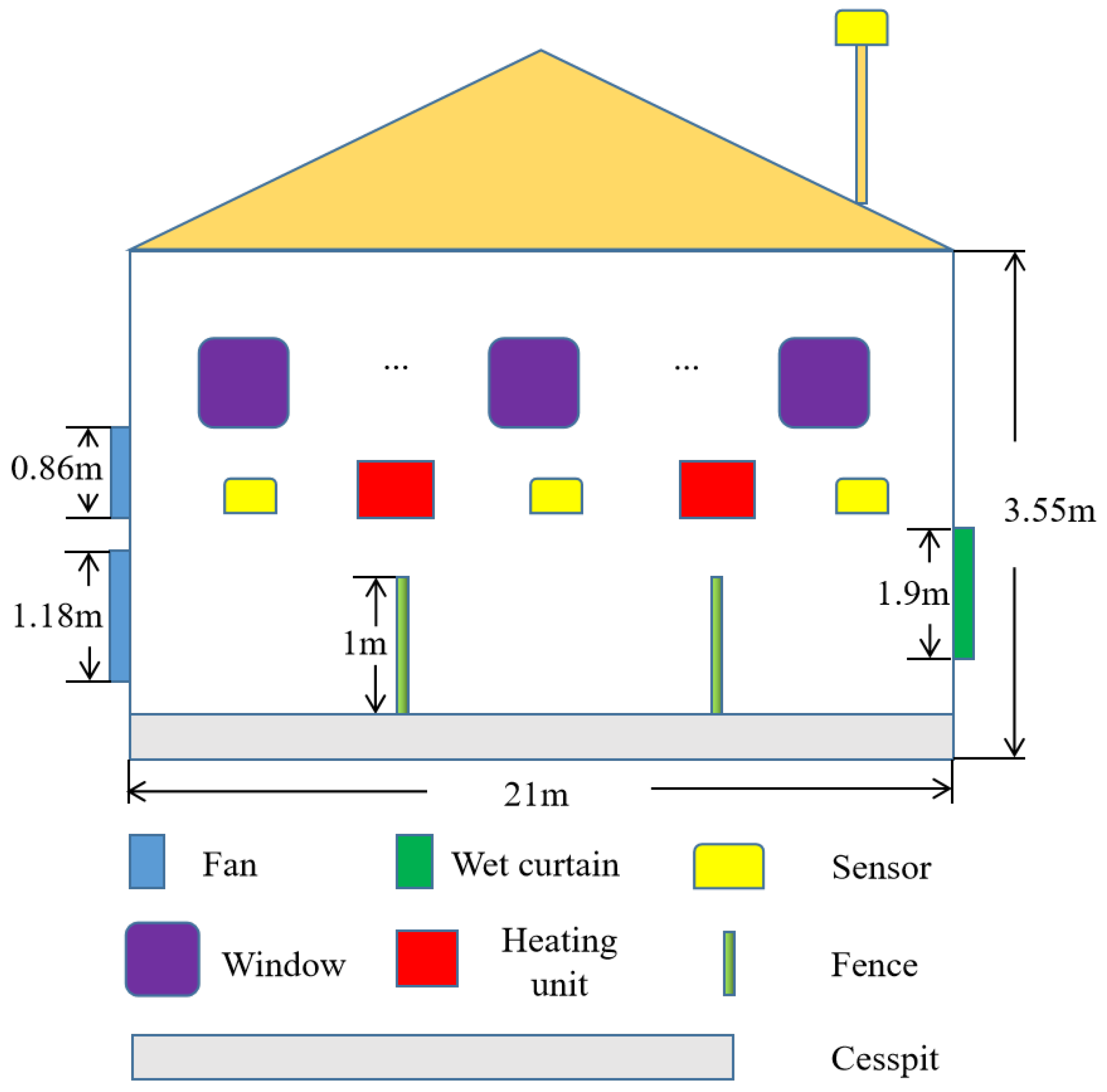
Figure 4 shows the cross-section of the experimental pig house. The pig house is oriented north to south with the wet curtains located on the east wall and the fans located on the west wall. The dimensions of the wet curtains are 1.83 m (width) × 1.9 m (height) × 0.15 m (thickness), and the bottom of the wet curtains is 0.68 m above the ground inside the house. There are a total of 2 fans with two different models. The dimensions of the large fan are 1.18 m × 1.18 m, whose power is between 0.75 and 1.15 kW, and the dimensions of the small fan are 0.86 m × 0.86 m, indicating power between 0.37 and 0.62 kW. The bottom of the large fans is 0.55 m and 0.63 m above the ground inside the house, respectively, while the bottom of the small fans is 0.85 m and 0.93 m above the ground inside the house, respectively. Inside the pig house, there is one HC2S3 sensor installed in each pen, and a heater is installed between two pens, whose power is between 5 and 20 kW.

2.3.4. Description of the Experimental Data

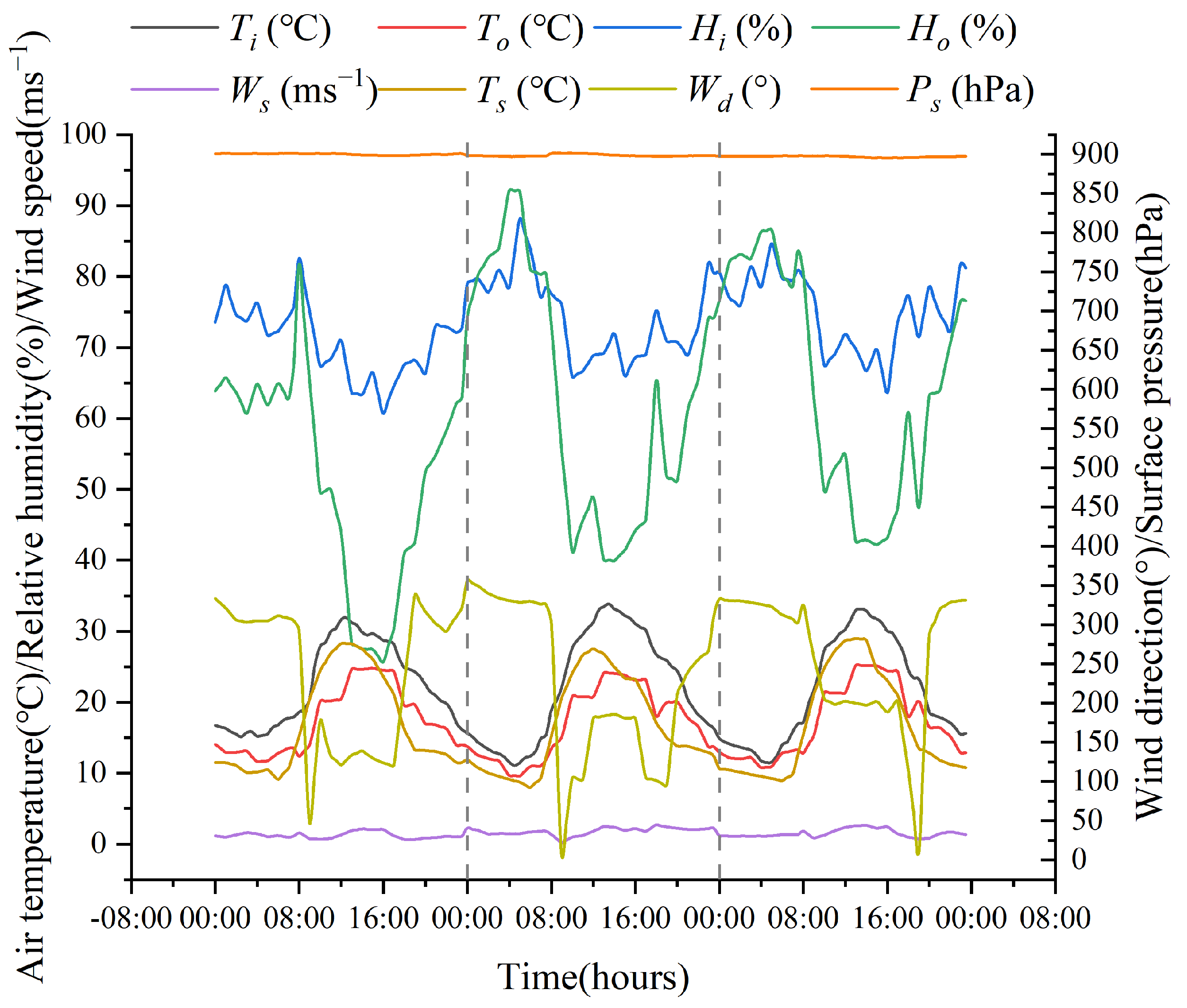
The total duration of the experiment was 4 months (from September 2022 to December 2022). At the beginning of the experiment (September 2022), the average age of the pigs in the experimental barn was about 47 days, and the average weight of each pig was 20–30 kg. At the end of the experiment (December 2022), the average weight of each pig was 100–110 kg, and four pigs died during the experiment with a mortality rate of about 2.53%. The amount of data collected over the four months totaled 5856 entries (5856 = 122 × 24 × 2), and the interval between two adjacent data is 30 min. These data include indoor air temperature $T_i$, outdoor air temperature $T_o$, indoor relative humidity $H_i$, outdoor relative humidity $H_o$, outdoor wind speed $W_s$, outdoor wind direction $W_d$, surface temperature $T_s$, surface pressure $P_s$ and control strategies. The indoor air temperature and indoor relative humidity are used to represent the environment inside the experimental pig house. The outdoor air temperature, outdoor relative humidity, outdoor wind speed, outdoor wind direction, surface temperature and surface pressure are used to represent the environment outside the experimental pig house, which can affect the environment inside the pig house. Control strategies are the ways in which temperature and humidity are regulated in the pig house, such as insulation, natural ventilation, mechanical ventilation, humidification, etc. In this study, the monitored data are processed by the three-way k-means model, and the new data are compared with each class cluster of clustering and assigned to the most appropriate class cluster, at which time the control method represented by that class cluster is the result of the model output. For example, if the temperature in the pig house is high during the day, the value of the air temperature attributed in the data input to the three-way k-means model will be larger, and it will be assigned to the class cluster that represents turning on the fan or increasing the power of the fan. Then, the output of the model will be the result of turning on the fan or increasing the power of the fan. At night, the temperature inside the pig house decreases, and then the model will regulate the indoor temperature by decreasing the fan power or turning on the heaters. Figure 5 shows the weather data for three days (26 September 2022 to 28 September 2022).

In the following month, the experiment of adjusting indoor temperature and humidity was carried out. The pigs in the experimental pig house are fattening pigs, the appropriate temperature for growth is 17–23 °C Celsius, and the optimal humidity is 65–70%. Sensors were used to measure the meteorological data inside and outside the pig house, which were then input into the k-means model. The k-means model processes the data and outputs a control strategy that adjusts the temperature and humidity in the pig house by adjusting the power of fans, wet curtains and heaters. After the control strategy was determined by the model, the temperature and humidity inside the pig house were checked every 15 s to see if they had returned to normal levels. If the temperature and humidity inside the pig house had not yet returned to normal levels, the current meteorological data were collected and fed back into the k-means model, which adjusted the power of the devices and continued running for another 15 s. This process was repeated until the temperature and humidity inside the pig house returned to normal levels.

2.3.5. Description of the Clustering Performance Experiments

To verify the performance of the clustering algorithm TWKS, we select six standard datasets from the UCI library to test the proposed algorithm. The UCI library is a dataset library common to the machine learning field, which is used to validate the performance of the algorithms in the machine learning domain. The specific dataset information is shown in

Table 1. Description of UCI datasets used in the clustering experiment.

Datasets Ratio	Samples	Attributes	Classes
Iris	140	4	3
Wine	178	13	3
Glass	214	9	7
Cancer	116	9	2
Sonar	208	60	2
Bank	1372	4	2

.

Then, some evaluation indicators will be presented below to assess the performance of the clustering algorithm.

Accuracy ($ACC$) is a commonly used external metric to evaluate the clustering performance, and the higher the accuracy, the better the clustering performance [42]. The accuracy is calculated as follows:

$$ACC=\frac{{\displaystyle \sum _{i=1}^{|{\theta }_P|}}max\left\{\right|{\theta }_P\cap {\theta }_C\left|\right\}}{N}$$

(11)

where N denotes the total number of samples, ${\theta }_P$ denotes the prediction result of three-way clustering, and ${\theta }_C$ denotes the correct result of the dataset. The $ACC$ calculated for the experiments of the three-way clustering algorithm in this paper is calculated using objects in the cluster core domain.

The Adjusted Rand Index ($ARI$) is a common external evaluation indicator for clustering, which measures the similarity between two clustering results by calculating the number of sample pairs assigned to the same or different clusters in the real labels and clustering results [43]. The calculation formula is as follows:

$$ARI=\frac{2(ad-bc)}{(a+b)(b+d)+(a+c)(c+d)}$$

(12)

where a denotes the number of sample pairs that belong to the same cluster in both real and predicted results. b denotes the number of sample pairs that belong to the same cluster in the real results but do not belong to the same cluster in the predicted results. c denotes the number of sample pairs that do not belong to the same cluster in the real results but belong to the same cluster in the predicted results, and d denotes the number of sample pairs that do not belong to the same cluster in both the real results and predicted results.

The average silhouette index ($AS$) is an internal indicator of clustering performance that reflects the clustering structure’s intra-class compactness and inter-class separateness [44]. The larger the average contour coefficient, the better the clustering performance. The average silhouette index is calculated as follows:

$$AS=\frac{1}{N}\sum _{i=1}^N{S}_i$$

(13)

where N denotes the total number of samples and $S_i$ is the silhouette index of the i-th sample.

$$S_i=\frac{b_i-a_i}{max(a_i,b_i)}$$

(14)

where $a_i$ is the intra-class similarity, which denotes the average distance between sample $x_i$ and other samples in the same cluster: the larger the value, the greater the likelihood that the sample belongs to the same cluster. $b_i$ is the degree of inter-class dissimilarity, which represents the minimum value of the average distance between sample $x_i$ and samples in other clusters: the larger the value, the less likely it is the sample belongs to other clusters.

2.3.6. Description of Control System Experiments

The experimental setup of the control system in this paper is divided into two parts. The first part is used to verify the effectiveness of the control system and compare it with a naturally ventilated pigsty without control (September 2022 to October 2022). The second part is used to verify the temperature control effect of the control system, compare it with a threshold-based control system, and evaluate it based on the length of temperature anomaly time (November 2022 to December 2022). Temperature anomaly time refers to the time within 24 h when the specified temperature is exceeded in the pigsty (the temperature range set in this paper is 17–23 °C).

To assess the system’s ability to prevent abnormal temperatures, we calculated the proportion of time spent in temperature abnormalities within the pig house on a daily basis.

$$P_{ab}=\frac{T_{ab}}{T}$$

(15)

where $P_{ab}$ denotes the percentage of time with temperature anomalies in a day, $T_{ab}$ denotes the time with temperature anomalies in a day, and T denotes the total time in a day (24 h).

3. Results and Discussions

3.1. Experimental Results of Abnormal Data Detection

To validate the accuracy of using the Isolation Forest algorithm for outlier detection, we added outlier values to the dataset at different proportions. We conducted 100 experiments in a Python environment for each proportion of outlier values.

Table 2. Description of datasets used in the experiment3.

Outliers Ratio	Temperature Accuracy	Humidity Accuracy
0∼1%	99.92%	98.89%
1∼3%	98.37%	97.99%
3∼5%	96.84%	95.26%
5∼10%	87.61%	83.44%

shows the average detection results of the isolation forest algorithm. It can be observed that when the proportion of outliers is less than or equal to 1%, the detection accuracy of temperature and humidity is almost 100% with negligible errors. When the proportion of outliers is between 1% and 3%, the detection accuracy of temperature and humidity is around 98%. When the proportion of outliers is between 3% and 5%, the detection accuracy of temperature and humidity can still remain above 95%. However, when the proportion of outliers increases from 5% to 10%, the performance of temperature and humidity detection deteriorates with accuracy ranging from 80% to 90%. In the actual process of temperature and humidity adjustment in pig houses, the abnormal rate of sensor data is basically below 3%. Therefore, the experimental results of the isolation forest algorithm align with expectations, and the next steps can be carried out on this basis.

3.2. Experimental Results of Clustering Performance

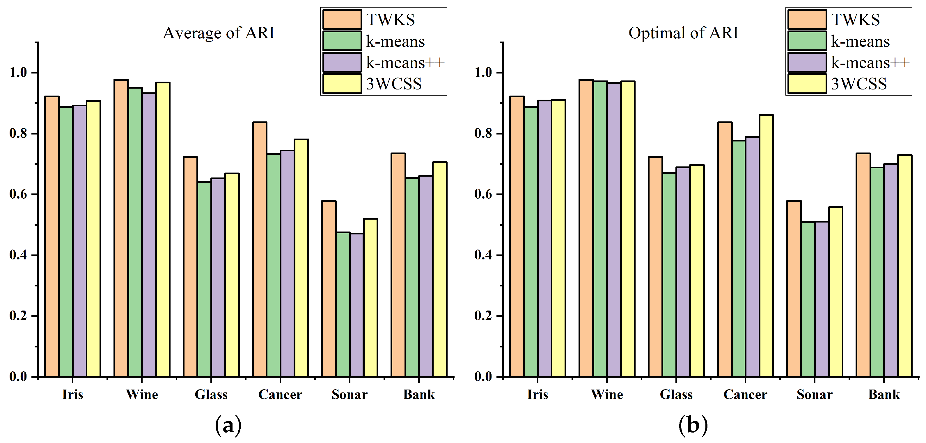
This paper compares the proposed TWKS algorithm with k-means, k-means++, and 3WCSS [45] in terms of $ACC$, $ARI$, and $AS$. The experiment is repeated 100 times for each dataset, and the average values of $ACC$, $ARI$, and $AS$ are calculated for each algorithm. The overall performance of the algorithms is compared based on these average values, while the best performance of each algorithm is determined based on the optimal values.

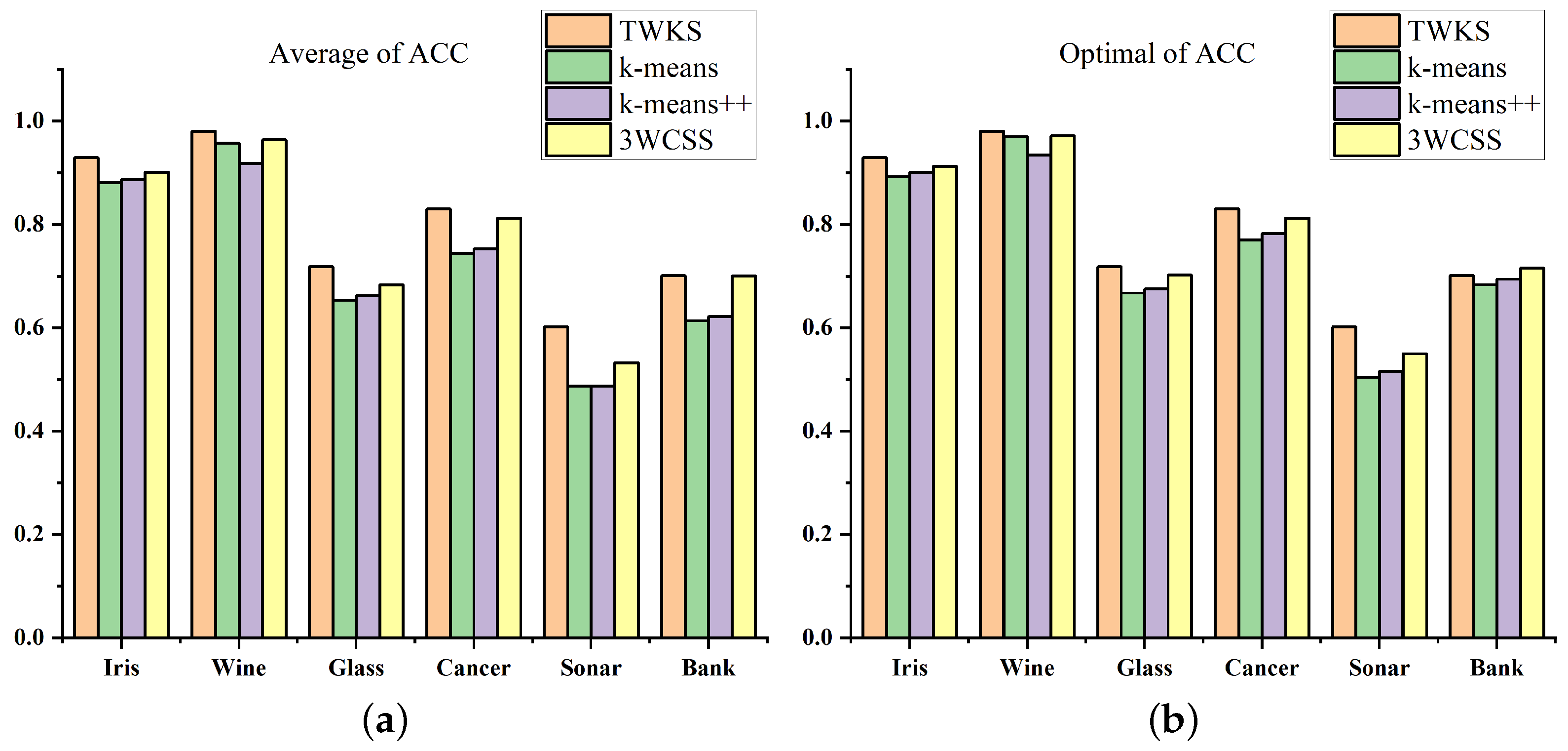
Figure 6a,b illustrate the average and best values of $ACC$, respectively. The graph clearly shows that the proposed TWKS algorithm outperforms the other algorithms in terms of both average and best $ACC$ values across all six datasets used in the experiment. This indicates that the proposed algorithm significantly improves the accuracy of the clustering results, leading to clustering results that are closer to the ground truth. This improvement is particularly valuable when constructing a temperature and humidity intelligent control system, as it helps reduce errors and enhance the precision of temperature and humidity control.

The average and best values of $ARI$ are depicted in Figure 7a,b, respectively. Figure 7a clearly demonstrates that the proposed TWKS algorithm achieves the highest average $ARI$ performance across all the datasets used in the experiment. Furthermore, Figure 7b illustrates that TWKS attains the best ARI values in five out of the six datasets, with slightly lower performance than the 3WCSS algorithm in the Cancer dataset. Thus, overall, the proposed TWKS algorithm significantly improves the similarity between the clustering results and the ground truth.

The average and best values of $AS$ are presented in Figure 8a,b, respectively. As depicted in the graph, it is evident that the proposed TWKS algorithm achieves the best performance in terms of both average and best $AS$ values for the majority of the datasets. This indicates that the TWKS algorithm effectively makes the clustering results more compact within clusters and more separated between clusters. Consequently, compared to the other three comparative algorithms, the proposed TWKS algorithm achieves higher intra-cluster similarity and produces superior clustering results.

Based on the analysis of the experimental results presented above, the proposed TWKS algorithm significantly improves the selection of initial cluster centers and enhances the quality of these centers compared to k-means, k-means++, and 3WCSS algorithms. As a result, the clustering results obtained using TWKS are more compact within clusters and exhibit the highest similarity to the ground truth, indicating their closer proximity to the actual results. Therefore, when utilizing the proposed TWKS algorithm to construct a k-means model for a temperature and humidity intelligent control system in pig houses, it can effectively reduce errors, enhance the accuracy of the model, and yield reasonable and precise control outcomes.

3.3. Experimental Results of Microclimate Control

3.3.1. Experimental Database

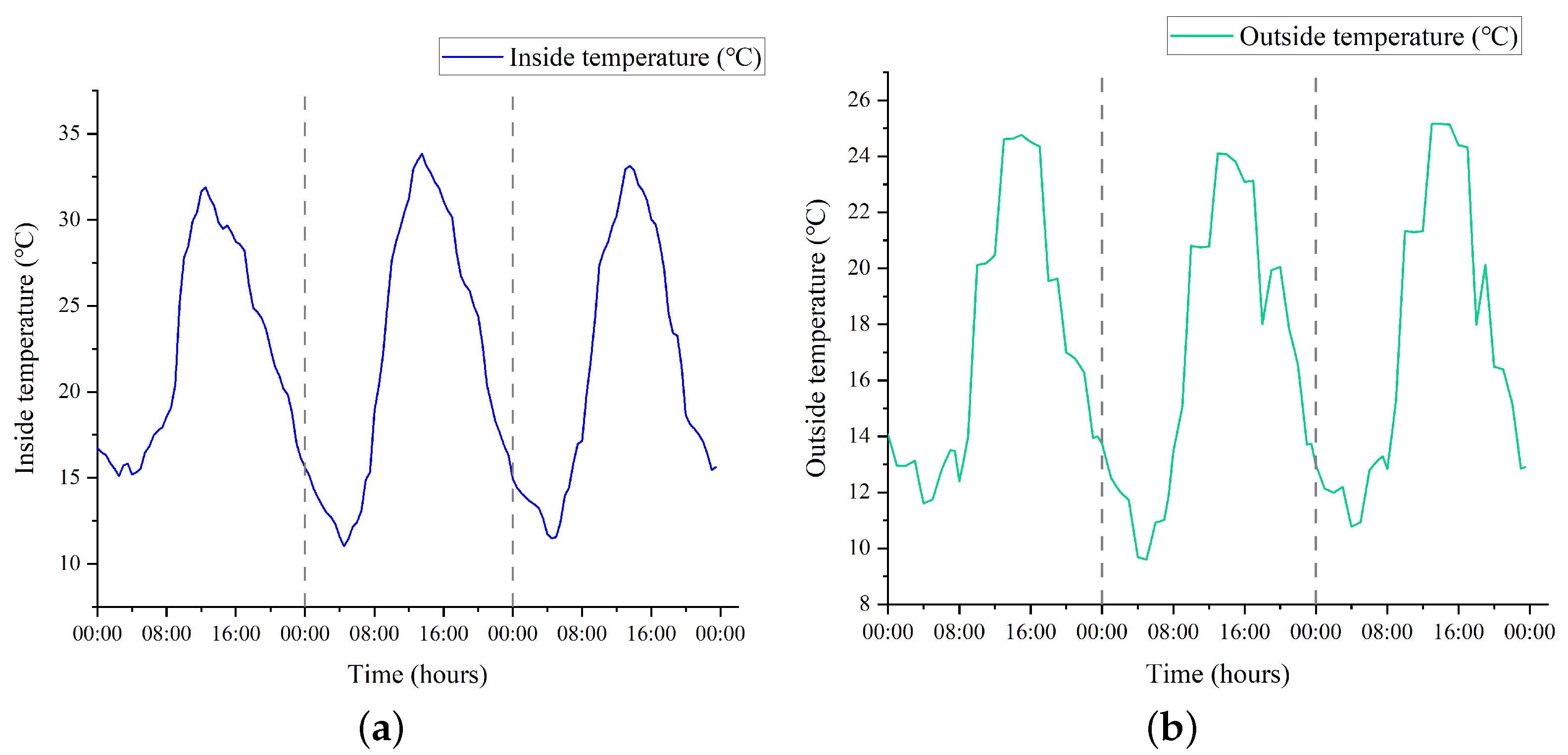
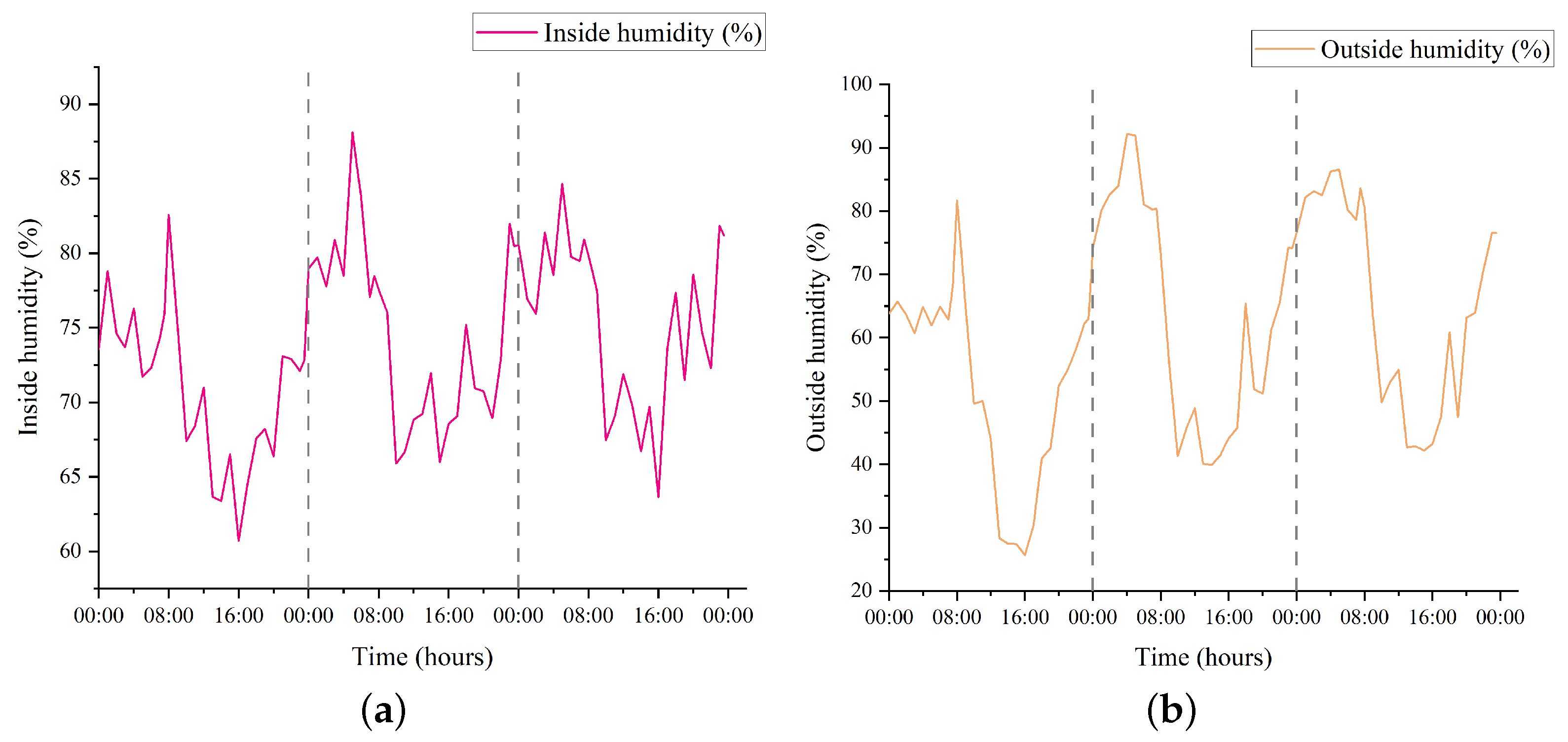
For this simulation, a real database is applied for four months. The database included the evolution of the indoor and outdoor climate conditions such as inside temperature (Figure 9a), the outside temperature (Figure 9b), the inside humidity (Figure 10a), the outside humidity (Figure 10b), the wind speed (Figure 11a), the wind direction (Figure 11b), the surface temperature (Figure 11c), and the surface pressure (Figure 11d).

3.3.2. Comparative Analyses of the Microclimate inside the Pig House without and with the Control

In this section, we compared the environmental conditions inside the pigsty using the control system proposed in this paper with those using natural ventilation without the control system. Figure 12 shows the evolution of the air temperature inside the pig house with and without the control system. From the graph, it can be observed that without temperature control in the pig house, the maximum and minimum temperatures exceed the suitable range for pig growth, and the temperature fluctuates significantly, which is detrimental to the healthy growth of the pigs. After implementing the intelligent control system designed in this study, the temperature variations in the pig house are reduced, maintaining the temperature within the optimal range for pig growth. By using the intelligent control system to analyze the monitored indoor air temperature, outdoor air temperature, indoor relative humidity, and other data, we dynamically adjust the output power of fans and heaters to maintain the temperature in the pig house within the range suitable for fattening pig growth (17–23 °C). Usually, during the day, the ventilation system starts working to reduce the indoor air temperature. At night, the heating system starts, raising the air temperature inside the pig house to around 18 °C. Therefore, through comparative analysis, it can be concluded that the intelligent control system designed in this study effectively maintains the temperature in the pig house, preventing excessive heat or cold, providing an appropriate temperature range for pig growth, and improving pig growth rate and welfare.

Figure 13 depicts the humidity variations inside the pig house with and without the utilization of a controller. The graph illustrates that in the absence of the control system, humidity levels in the pig house fluctuated between 60% and 85%, exhibiting a wide range of variation. Notably, between 11 a.m. and 2 p.m., humidity reached higher values, coinciding with elevated temperatures within the pig house. This combination of high temperature and humidity could have detrimental effects on the pigs’ healthy growth. Pigs are particularly sensitive to humidity, and the range of humidity observed in the pig house without a controller does not meet their growth requirements [46]. However, upon implementing the intelligent control system proposed in this study, the amplitude of humidity fluctuations in the pig house decreased, approaching a state of stability. Overall, the humidity levels were maintained within the range of 65% to 70%, aligning with the optimal growth requirements for pigs. By leveraging the intelligent control system, the magnitude of humidity fluctuations within the pig house was reduced, effectively mitigating constraints on pig growth caused by significant environmental humidity variations.

3.3.3. Comparative Analyses of the Temperature inside the Pig House with Threshold-Based Controller

In this section, we compared the temperature anomaly time inside the pig house using the control system proposed in this paper with a traditional threshold-based system [33]. In different animal husbandry buildings, the threshold of the control system will vary depending on the animals being raised. In this experiment, the upper limit of the temperature threshold is set to 23 °C, the lower limit is set to 17 °C, the upper limit of the relative humidity threshold is set to 70%, and the lower limit is set to 65%.

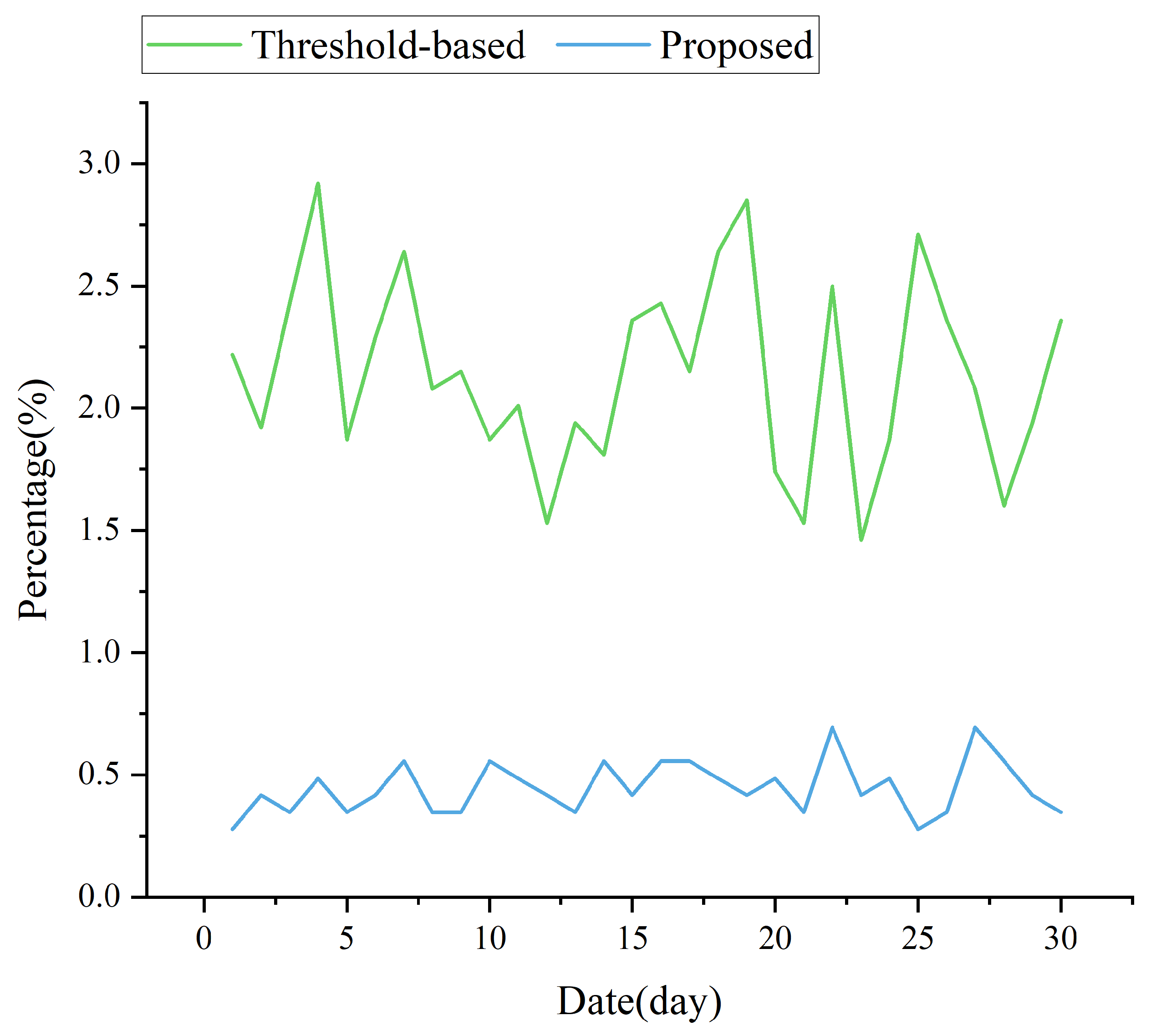
Figure 14 illustrates the comparison between the two controllers in terms of the proportion of abnormal time. The graph demonstrates that over a period of 30 days, when utilizing the threshold-based controller, the maximum proportion of abnormal time in a day was 2.92%, the minimum was 1.46%, and the average was 1.89%. In contrast, when employing our designed controller, the maximum proportion of abnormal time in a day was 0.694%, the minimum was 0.278%, and the average was 0.447%. The experimental results reveal that under the regulation of our designed controller, the pig house experienced an average of only about 6 min of abnormal temperature time per day. In contrast, when regulated by the threshold-based controller, the pig house encountered an average of approximately 27 min of abnormal temperature time per day. This significant reduction in the duration of abnormal temperature periods greatly diminishes the likelihood of pigs falling ill due to temperature fluctuations and provides a suitable environment for their growth [16].

4. Limitations

Several limitations of the present study should be noticed. Firstly, the model designed in this study did not decouple temperature and humidity, so controlling temperature may have some impact on humidity. Similarly, dehumidification or humidification operations may also lead to an increase or decrease in temperature. Under such mutual influence, the precision of the model’s regulation of temperature and humidity in the pigsty is slightly reduced, and the probability of temperature and humidity abnormalities increases.

Secondly, there are redundant sensors in the pigsty, which leads to redundant data collected by the sensors, increases the computational load of the model, and affects the speed of the model. The presence of a large number of redundant sensors not only increases economic costs but also prevents the effective utilization of data from sensors in optimal positions. Additionally, there is a large error between the measured data, which is not conducive to the precise control of temperature and humidity in the pigsty.

5. Conclusions

Maintaining optimal temperature and humidity levels within pig houses is essential for fostering ideal conditions for pig growth. To address this issue, we have developed and implemented an enhanced temperature and humidity intelligent control system within a pig house. This system integrates a three-way decision and clustering algorithm, encompassing key modules such as data preprocessing, k-means model training, and the regulation of indoor air temperature and relative humidity. In the data preprocessing module, we employ the isolation forest algorithm to detect outliers within the dataset, achieving a remarkable accuracy rate of 98%. When constructing the k-means model, we enhance precision by integrating three decision rules and sample stability into the k-means algorithm. This augmentation substantially improves the model’s classification performance when handling weather data. The controller module subsequently analyzes the clustering results produced by the k-means model, enabling the determination of the most suitable control strategy. This process involves the activation or deactivation of specific devices to maintain an optimal environment within the pig house. The controller efficiently sustains a consistent relative humidity level of 65% to 70% while adjusting indoor air temperature to 16 °C during the night and 25 °C during the day. Experimental findings underscore the effectiveness of our proposed system in regulating temperature and humidity within the pig house, resulting in a notable reduction in the duration of temperature anomalies.

In summary, the intelligent temperature and humidity control system outlined in this paper, rooted in the three-way decision and clustering algorithm, has been validated through experiments conducted within the pig house. These results demonstrate the feasibility of implementing the three-way decision and clustering algorithm in temperature and humidity control systems. Importantly, the applicability of the control system is not limited to the specific experimental pigsties studied but extends to a wide range of livestock buildings, including chicken coops, cowsheds, and more.

References

1. Quiniou, N.; Noblet, J.; van Milgen, J.; Dubois, S. Modelling heat production and energy balance in group-housed growing pigs exposed to low or high ambient temperatures. Br. J. Nutr. 2001, 85, 97–106. [Google Scholar] [CrossRef] [PubMed]
2. Gautam, K.R.; Rong, L.; Zhang, G.Q.; Bjerg, B.S. Temperature distribution in a finisher pig building with hybrid ventilation. Biosyst. Eng. 2020, 200, 123–137. [Google Scholar] [CrossRef]
3. Mun, H.S.; Rathnayake, D.; Dilawar, M.A.; gil Jeong, M.; Yang, C.J. Effect of ambient temperature on growth performances, carcass traits and meat quality of pigs. J. Appl. Anim. Res. 2022, 50, 103–108. [Google Scholar] [CrossRef]
4. Morales, A.; Cota, S.E.M.; Ibarra, N.O.; Arce, N.; Htoo, J.K.; Cervantes, M. Effect of heat stress on the serum concentrations of free amino acids and some of their metabolites in growing pigs. J. Anim. Sci. 2016, 94, 2835–2842. [Google Scholar] [CrossRef] [PubMed]
5. Hörtenhuber, S.J.; Schauberger, G.; Mikovits, C.; Schönhart, M.; Baumgartner, J.; Niebuhr, K.; Piringer, M.; Anders, I.; Andre, K.; Hennig-Pauka, I.; et al. The Effect of Climate Change-Induced Temperature Increase on Performance and Environmental Impact of Intensive Pig Production Systems. Sustainability 2020, 12, 9442. [Google Scholar] [CrossRef]
6. Seidel, D.S.; Field, T.C.; Schinckel, A.P.; Stwalley, C.S.; Stwalley, R.M. Effects of temperature probe orientation on the Purdue hog cooling pad data acquisition. Comput. Electron. Agric. 2020, 175, 105609. [Google Scholar] [CrossRef]
7. St-Pierre, N.; Cobanov, B.; Schnitkey, G. Economic Losses from Heat Stress by US Livestock Industries. J. Dly. Sci. 2003, 86, 52–77. [Google Scholar] [CrossRef]
8. Wang, M.Q.; Li, X.; Larsen, M.L.V.; Liu, D.; Rault, J.L.; Norton, T. A computer vision-based approach for respiration rate monitoring of group housed pigs. Comput. Electron. Agric. 2023, 210, 107899. [Google Scholar] [CrossRef]
9. Cao, M.B.; Zong, C.; Zhuang, Y.R.; Teng, G.H.; Zhou, S.N.; Yang, T. Modeling of Heat Stress in Sows Part 2: Comparison of Various Thermal Comfort Indices. Animals 2021, 11, 1498. [Google Scholar] [CrossRef]
10. Gourdine, J.L.; Rauw, W.M.; Gilbert, H.; Poullet, N. The Genetics of Thermoregulation in Pigs: A Review. Front. Vet. Sci. 2021, 8, 770480. [Google Scholar] [CrossRef]
11. Li, H.; Li, R.; Zhang, G.Q. Numerical study on the convective heat transfer of fattening pig in groups in a mechanical ventilated pig house. Comput. Electron. Agric. 2018, 149, 90–100. [Google Scholar] [CrossRef]
12. Kim, B.; Reddy, K.E.; Kim, H.R.; Kim, K.H.; Lee, Y.; Kim, M.; Ji, S.Y.; Lee, S.D.; Jeong, J.Y. Effects of recovery from short-term heat stress exposure on feed intake, plasma amino acid profiles, and metabolites in growing pigs. J. Anim. Sci. Technol. 2021, 63, 531–544. [Google Scholar] [CrossRef] [PubMed]
13. Yeo, U.H.; Lee, I.B.; Kim, R.W.; Lee, S.Y.; Kim, J.G. Computational fluid dynamics evaluation of pig house ventilation systems for improving the internal rearing environment. Biosyst. Eng. 2019, 186, 259–278. [Google Scholar] [CrossRef]
14. Sun, G.D.; Song, X.; Zou, Y.B.; Teng, T.; Jiang, L.; Shi, B.M. Dietary Glucose Ameliorates Impaired Intestinal Development and Immune Homeostasis Disorders Induced by Chronic Cold Stress in Pig Model. Int. J. Mol. Sci. 2022, 23, 7730. [Google Scholar] [CrossRef]
15. Yang, Y.W.; Chen, N.X.; Sun, L.; Zhang, Y.; Wu, Y.B.; Wang, Y.; Liao, X.D.; Mi, J.D. Short-term cold stress can reduce the abundance of antibiotic resistance genes in the cecum and feces in a pig model. J. Hazard. Mater. 2021, 416, 125868. [Google Scholar] [CrossRef]
16. Jin, H.; Meng, G.; Pan, Y.Z.; Zhang, X.; Wang, C.D. An Improved Intelligent Control System for Temperature and Humidity in a Pig House. Agriculture 2022, 12, 1987. [Google Scholar] [CrossRef]
17. Shin, H.; Kwak, Y.; Jo, S.K.; Kim, S.H.; Huh, J.H. Development of an optimal mechanical ventilation system control strategy based on weather forecasting data for outdoor air cooling in livestock housing. Energy 2023, 268, 126649. [Google Scholar] [CrossRef]
18. Cao, M.B.; Zong, C.; Wang, X.S.; Teng, G.H.; Zhuang, Y.R.; Lei, K.D. Numerical simulations of airflow and convective heat transfer of a sow. Biosyst. Eng. 2020, 200, 23–39. [Google Scholar] [CrossRef]
19. Schauberger, G.; Schönhart, M.; Zollitsch, W.; Hörtenhuber, S.J.; Kirner, L.; Mikovits, C.; Baumgartner, J.; Piringer, M.; Knauder, W.; Anders, I.; et al. Economic Risk Assessment by Weather-Related Heat Stress Indices for Confined Livestock Buildings: A Case Study for Fattening Pigs in Central Europe. Agriculture 2021, 11, 122. [Google Scholar] [CrossRef]
20. Licharz, H.; Rösmann, P.; Krommweh, M.S.; Mostafa, E.; Büscher, W. Energy Efficiency of a Heat Pump System: Case Study in Two Pig Houses. Energies 2020, 13, 662. [Google Scholar] [CrossRef]
21. Gomes, J.; Esteves, I.; Graciano Neto, V.V.; David, J.M.N.; Braga, R.; Arbex, W.; Kassab, M.; de Oliveira, R.F. A scientific software ecosystem architecture for the livestock domain. Inf. Softw. Technol. 2023, 160, 107240. [Google Scholar] [CrossRef]
22. Havelka, Z.; Kunes, R.; Kononets, Y.; Stokes, J.E.; Smutny, L.; Olsan, P.; Kresan, J.; Stehlik, R.; Bartos, P.; Xiao, M.; et al. Technology of Microclimate Regulation in Organic and Energy-Sustainable Livestock Production. Agriculture 2022, 12, 1563. [Google Scholar] [CrossRef]
23. Huang, T.; Zhang, G.Q.; Brandt, P.; Bjerg, B.; Pedersen, P.; Rong, L. An effective temperature derived from a mechanistic thermophysiological model for sows reared in hot climates. Biosyst. Eng. 2022, 220, 19–38. [Google Scholar] [CrossRef]
24. Costantino, A.; Fabrizio, E.; Ghiggini, A.; Bariani, M. Climate control in broiler houses: A thermal model for the calculation of the energy use and indoor environmental conditions. Energy Build. 2018, 169, 110–126. [Google Scholar] [CrossRef]
25. Kpodo, K.R.; Duttlinger, A.W.; Maskal, J.M.; McConn, B.R.; Johnson, J.S. Effects of Feed Removal during Acute Heat Stress on the Cytokine Response and Short-Term Growth Performance in Finishing Pigs. Animals 2021, 11, 205. [Google Scholar] [CrossRef] [PubMed]
26. Kroscher, K.A.; Fausnacht, D.W.; McMillan, R.P.; El-Kadi, S.W.; Wall, E.H.; Bravo, D.M.; Rhoads, R.P. Supplementation with artificial sweetener and capsaicin alters metabolic flexibility and performance in heat-stressed and feed-restricted pigs. J. Anim. Sci. 2022, 100, skac195. [Google Scholar] [CrossRef] [PubMed]
27. Ulpiani, G.; Borgognoni, M.; Romagnoli, A.; Di Perna, C. Comparing the performance of on/off, PID and fuzzy controllers applied to the heating system of an energy-efficient building. Energy Build. 2016, 116, 1–17. [Google Scholar] [CrossRef]
28. Xie, Q.; Su, Z.; Ni, J.; Zheng, P. Control system design and control strategy of multiple environmental factors in confined swine building. Trans. Chin. Soc. Agric. Eng. 2017, 33, 163–170. [Google Scholar]
29. Gao, L.A.; Er, M.W.; Li, L.H.; Wen, P.; Jia, Y.C.; Huo, L.M. Microclimate environment model construction and control strategy of enclosed laying brooder house. Poult. Sci. 2022, 101, 101843. [Google Scholar] [CrossRef]
30. Xie, Q.J.; Ni, J.Q.; Bao, J.; Su, Z.B. A thermal environmental model for indoor air temperature prediction and energy consumption in pig building. Build. Environ. 2019, 161, 106238. [Google Scholar] [CrossRef]
31. Li, B.; Wang, Y.; Zheng, W.; Tong, Q. Research progress in environmental control key technologies, facilities and equipment for laying hen production in China. Trans. Chin. Soc. Agric. Eng. 2020, 36, 212–221. [Google Scholar]
32. Tikhomirov, D.A.; Trunov, S.S.; Kuzmichev, A.V.; Rastimeshin, S.; Shepovalova, O. Energy-efficient thermoelectric unit for microclimate control on cattle breeding premises. Energy Rep. 2020, 6, 293–305. [Google Scholar] [CrossRef]
33. Du, Q.; Miao, Y.; Zhang, Y. Design of intelligent monitoring system of chicken house environment based on single-chip microcomputer. MATEC Web Conf. 2018, 227, 02008. [Google Scholar] [CrossRef]
34. Li, F.J.; Qian, Y.H.; Wang, J.T.; Dang, C.Y.; Jing, L.P. Clustering ensemble based on sample’s stability. Artif. Intell. 2019, 273, 37–55. [Google Scholar] [CrossRef]
35. Otsu, N. A Threshold Selection Method from Gray-Level Histograms. Automatica 1975, 11, 23–27. [Google Scholar] [CrossRef]
36. Naghavi Nozad, S.A.; Amir Haeri, M.; Folino, G. SDCOR: Scalable density-based clustering for local outlier detection in massive-scale datasets. Knowl.-Based Syst. 2021, 228, 107256. [Google Scholar] [CrossRef]
37. Abhaya, A.; Patra, B.K. RDPOD: An unsupervised approach for outlier detection. Neural Comput. Appl. 2022, 34, 1065–1077. [Google Scholar] [CrossRef]
38. Toller, M.B.; Geiger, B.C.; Kern, R. Cluster Purging: Efficient Outlier Detection Based on Rate-Distortion Theory. IEEE Trans. Knowl. Data Eng. 2023, 35, 1270–1282. [Google Scholar] [CrossRef]
39. Huang, J.W.; Zhong, M.X.; Jaysawal, B.P. TADILOF: Time Aware Density-Based Incremental Local Outlier Detection in Data Streams. Sensors 2020, 20, 5829. [Google Scholar] [CrossRef]
40. Riahi-Madvar, M.; Akbari Azirani, A.; Nasersharif, B.; Raahemi, B. A new density-based subspace selection method using mutual information for high dimensional outlier detection. Knowl.-Based Syst. 2021, 216, 106733. [Google Scholar] [CrossRef]
41. Hariri, S.; Kind, M.C.; Brunner, R.J. Extended Isolation Forest. IEEE Trans. Knowl. Data Eng. 2021, 33, 1479–1489. [Google Scholar] [CrossRef]
42. Guo, Q.H.; Yin, Z.Y.; Wang, P.X. An Improved Three-Way K-Means Algorithm by Optimizing Cluster Centers. Symmetry 2022, 14, 1821. [Google Scholar] [CrossRef]
43. Jiang, C.M.; Li, Z.C.; Yao, J.T. A shadowed set-based three-way clustering ensemble approach. Int. J. Mach. Learn. Cybern. 2022, 13, 2545–2558. [Google Scholar] [CrossRef]
44. Rousseeuw, P.J. Silhouettes: A graphical aid to the interpretation and validation of cluster analysis. J. Comput. Appl. Math. 1987, 20, 53–65. [Google Scholar] [CrossRef]
45. Wang, P.X.; Yang, X.B. Three-Way Clustering Method Based on Stability Theory. IEEE Access 2021, 9, 33944–33953. [Google Scholar] [CrossRef]
46. Kim, J.G.; Lee, S.Y.; Lee, I.B. The Development of an LSTM Model to Predict Time Series Missing Data of Air Temperature inside Fattening Pig Houses. Agriculture 2023, 13, 795. [Google Scholar] [CrossRef]
Figure 1. Blocks diagram of the pattern of black box used to choose the control scheme.
Agriculture 13 02020 g001
Figure 2. Flow chart of microcosmic regulation of temperature and humidity. K N N denotes the k-nearest neighbor algorithm.
Agriculture 13 02020 g002
Figure 3. Temperature and humidity control system block diagram.
Agriculture 13 02020 g003
Figure 4. Cross-sectional view of experimental pig house.
Agriculture 13 02020 g004
Figure 5. Results of the weather station (26 September 2022 to 28 September 2022). T i : indoor air temperature, T o : outdoor air temperature, H i : indoor relative humidity, H o : outdoor relative humidity, W s : wind speed, T s : surface temperature, W d : wind direction, P s : surface pressure.
Agriculture 13 02020 g005
Figure 6. A C C of each algorithms. (a): Average of A C C , (b): Optimal of A C C .
Agriculture 13 02020 g006
Figure 7. A R I of each algorithms. (a): Average of A R I , (b): Optimal of A R I .
Agriculture 13 02020 g007
Figure 8. A S of each algorithms. (a): Average of A S , (b): Optimal of A S .
Agriculture 13 02020 g008
Figure 9. Temperature conditions (26 September 2022 to 28 September 2022). (a): Inside temperature, (b): Outside temperature.
Agriculture 13 02020 g009
Figure 10. Humidity conditions (26 September 2022 to 28 September 2022). (a): Inside humidity, (b): Outside humidity.
Agriculture 13 02020 g010
Figure 11. The external climate conditions (26 September 2022 to 28 September 2022). (a): Wind speed, (b): Wind direction, (c): Surface temperature, (d): Surface pressure.
Agriculture 13 02020 g011
Figure 12. Comparison of inside temperatures with control and without control (26 September 2022 to 28 September 2022).
Agriculture 13 02020 g012
Figure 13. Comparison of inside humidity with control and without control (26 September 2022 to 28 September 2022).
Agriculture 13 02020 g013
Figure 14. Percentage of abnormal time in a day.
Agriculture 13 02020 g014