
Path Planning and Control System Design of an Unmanned Weeding Robot


Abstract
:1. Introduction
2. Materials and Methods
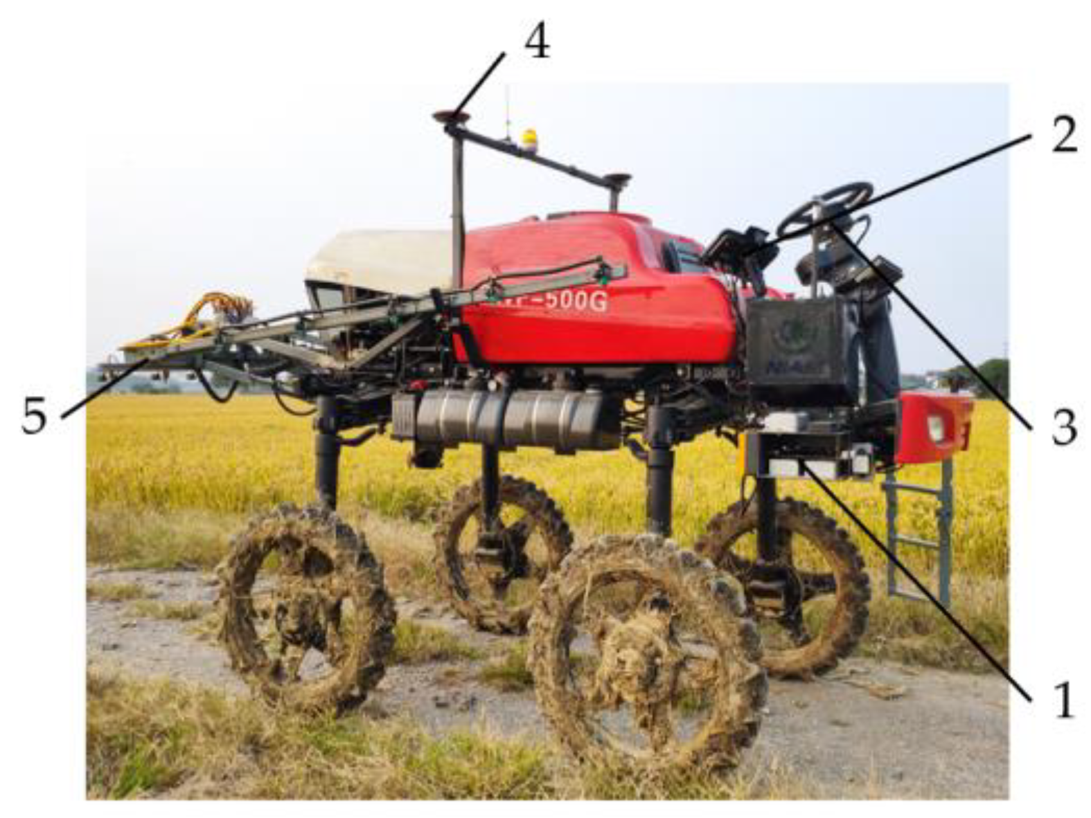
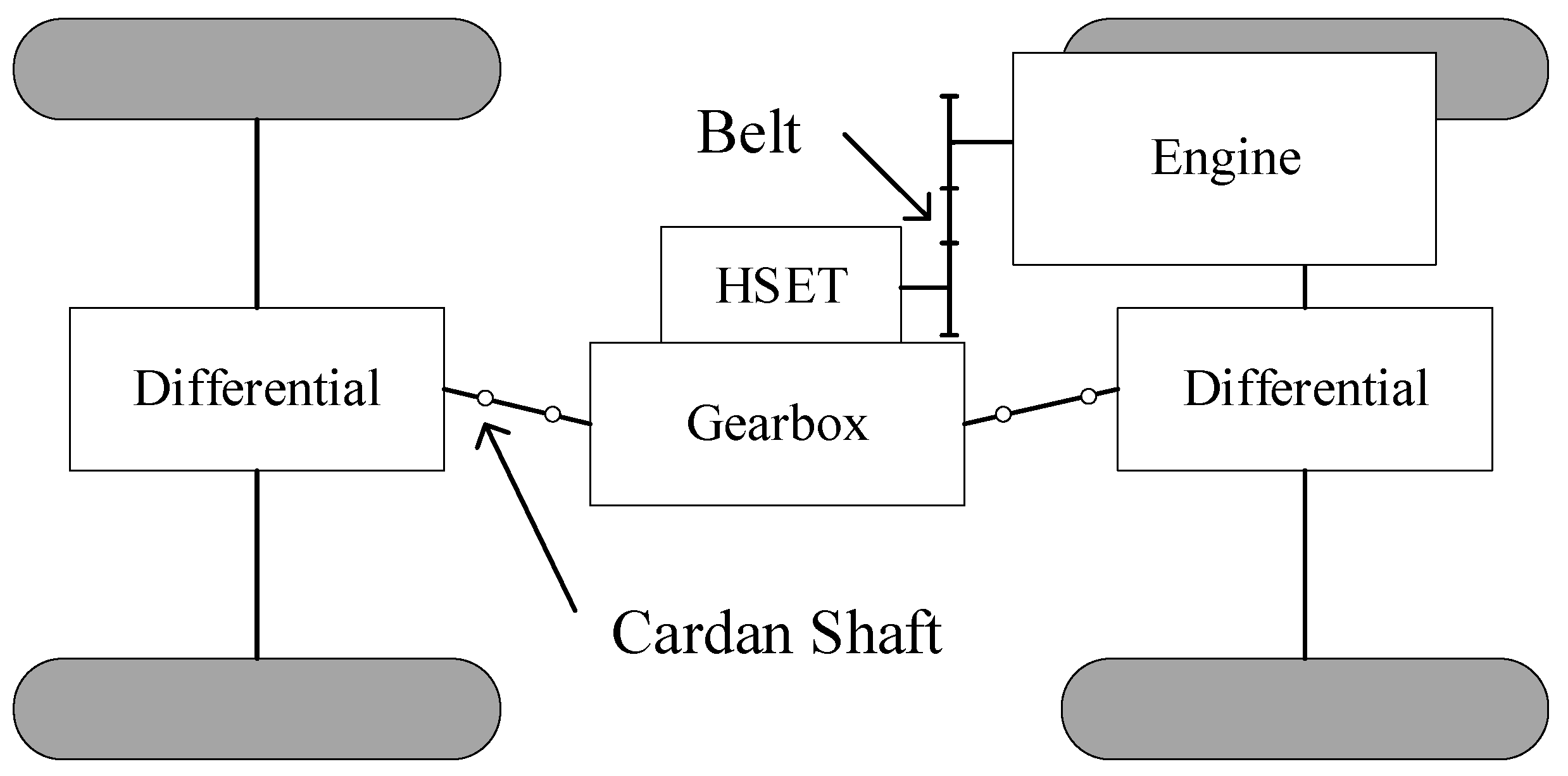
2.1. Composition of Weeding Robot
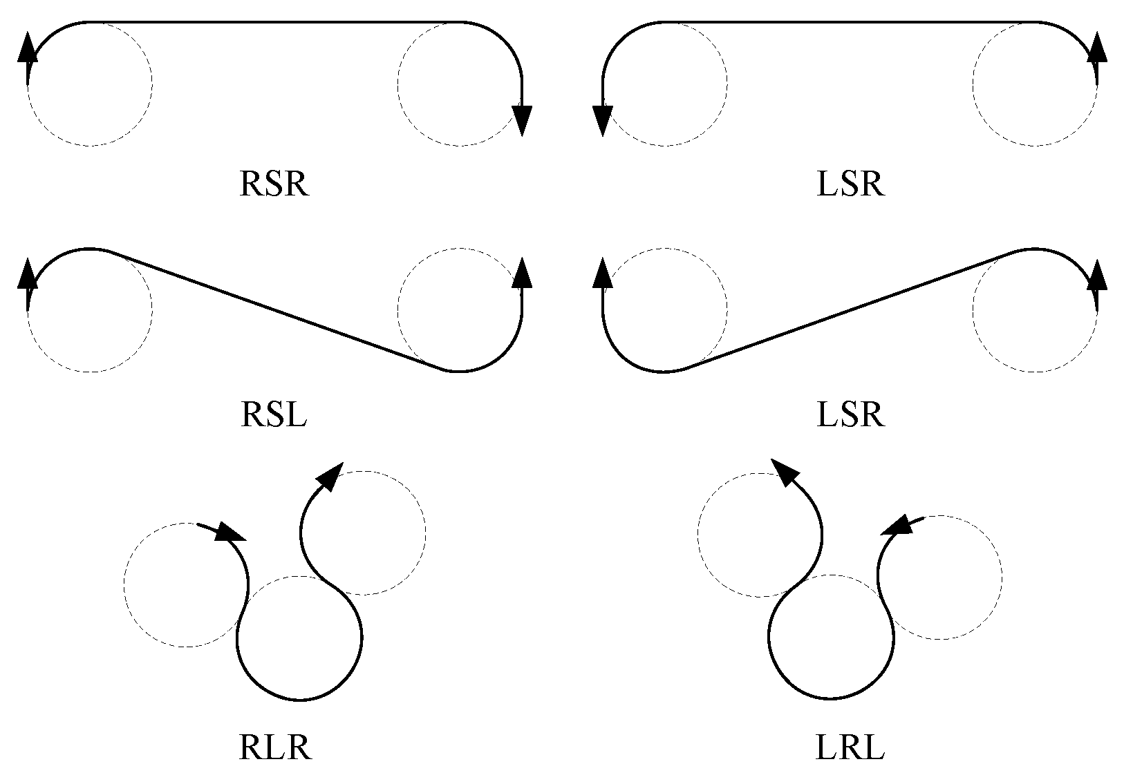
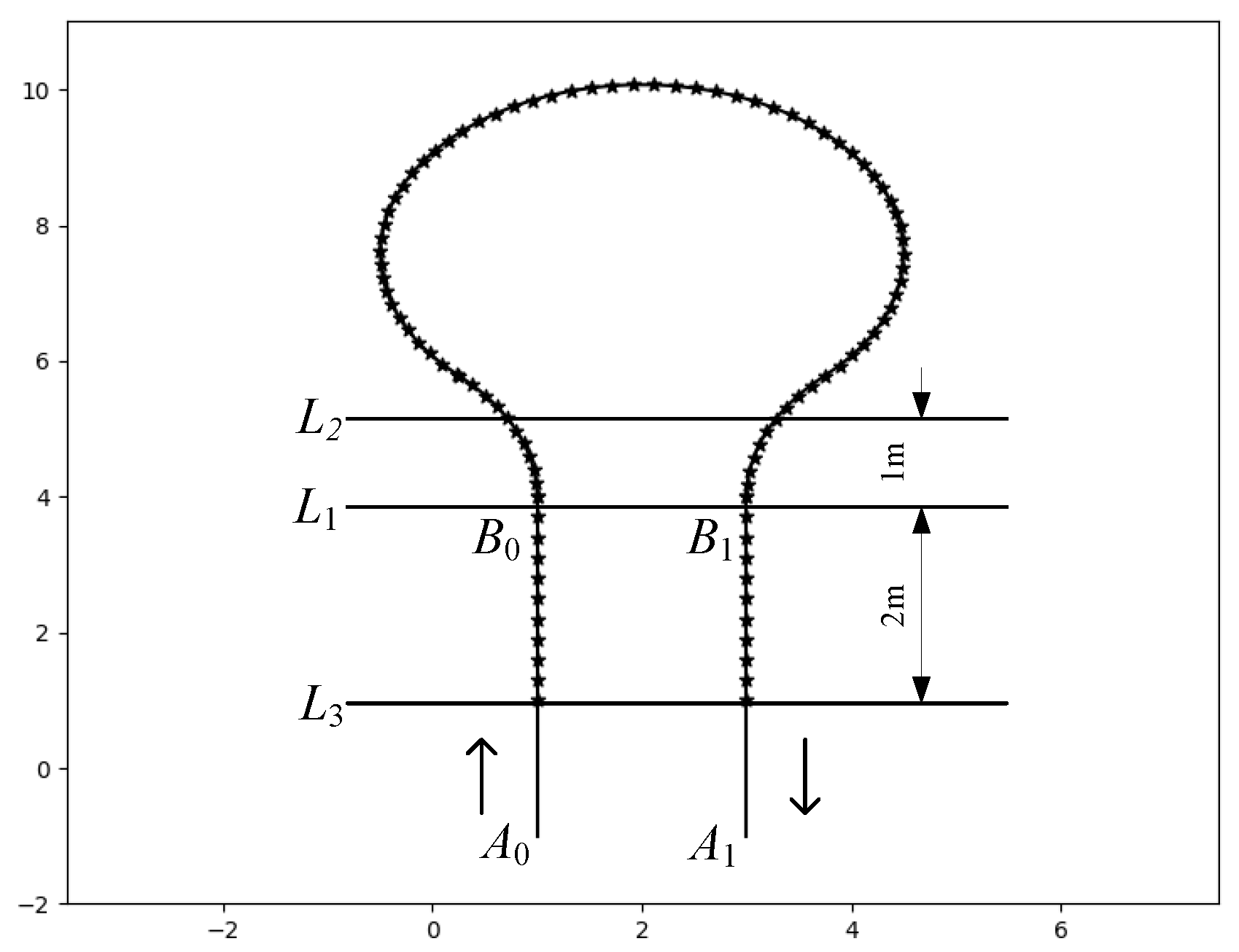
2.2. Path Planning
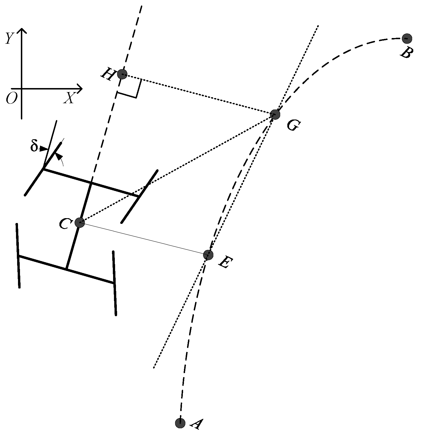
2.3. Path Tracing
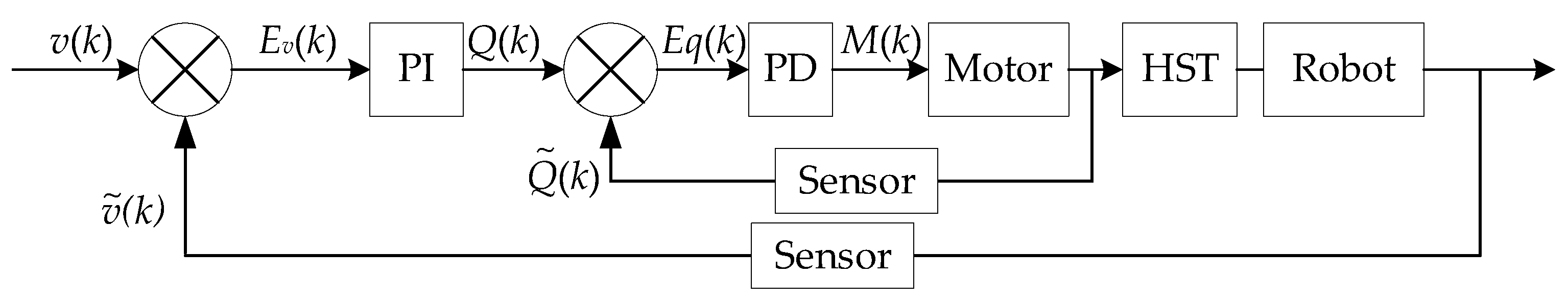
2.4. Speed Control System
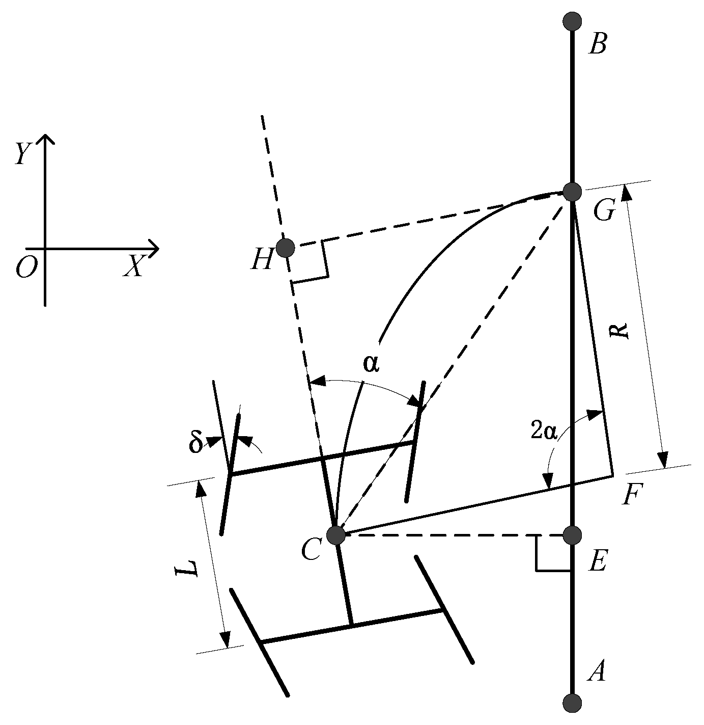
2.5. Steering Control System
2.6. Dataset Production
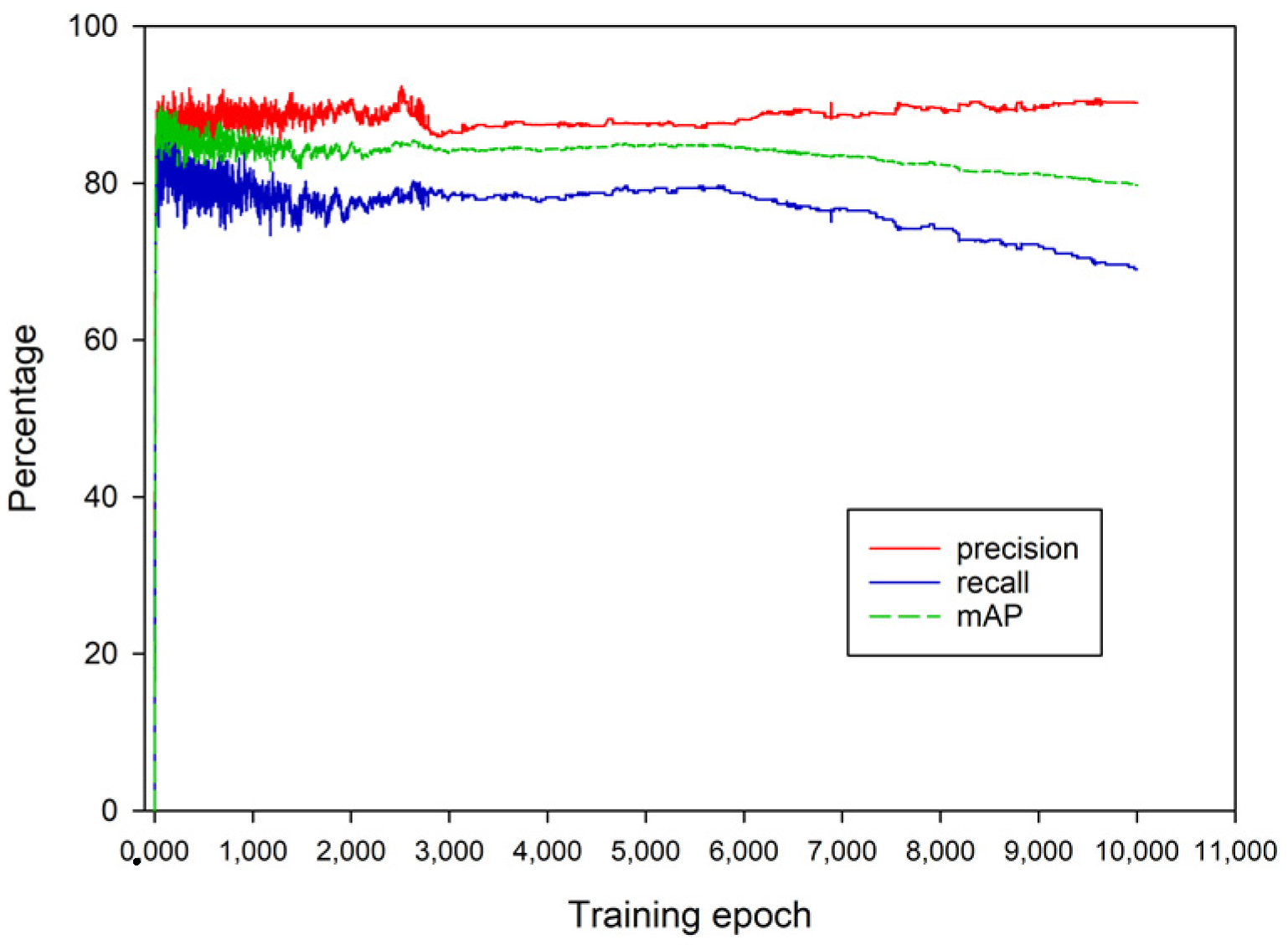
2.7. Model Building and Training
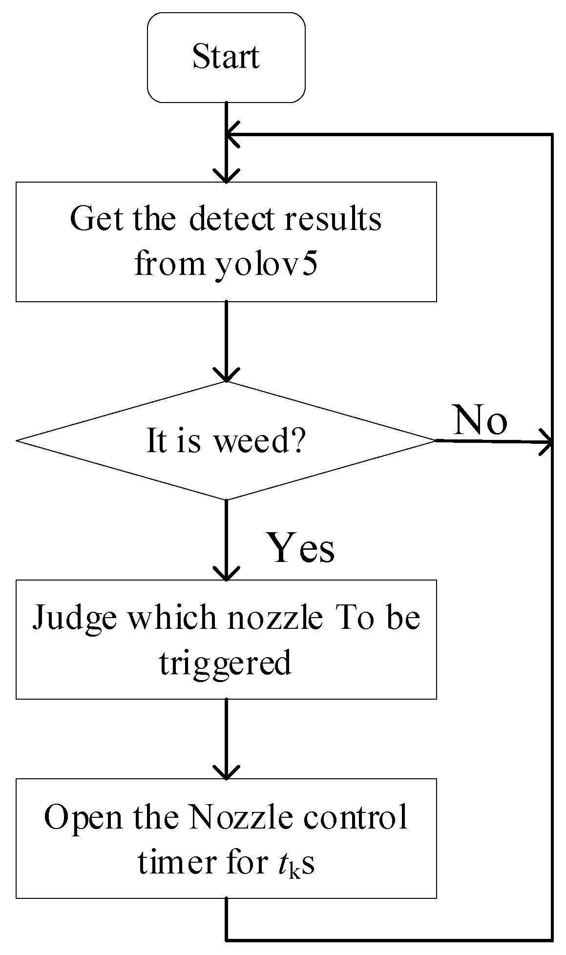
2.8. Weeding Decision Method
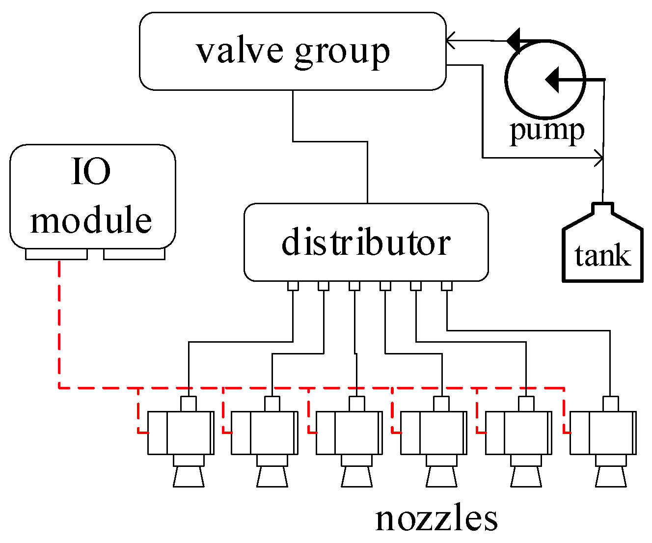
2.9. Spray System
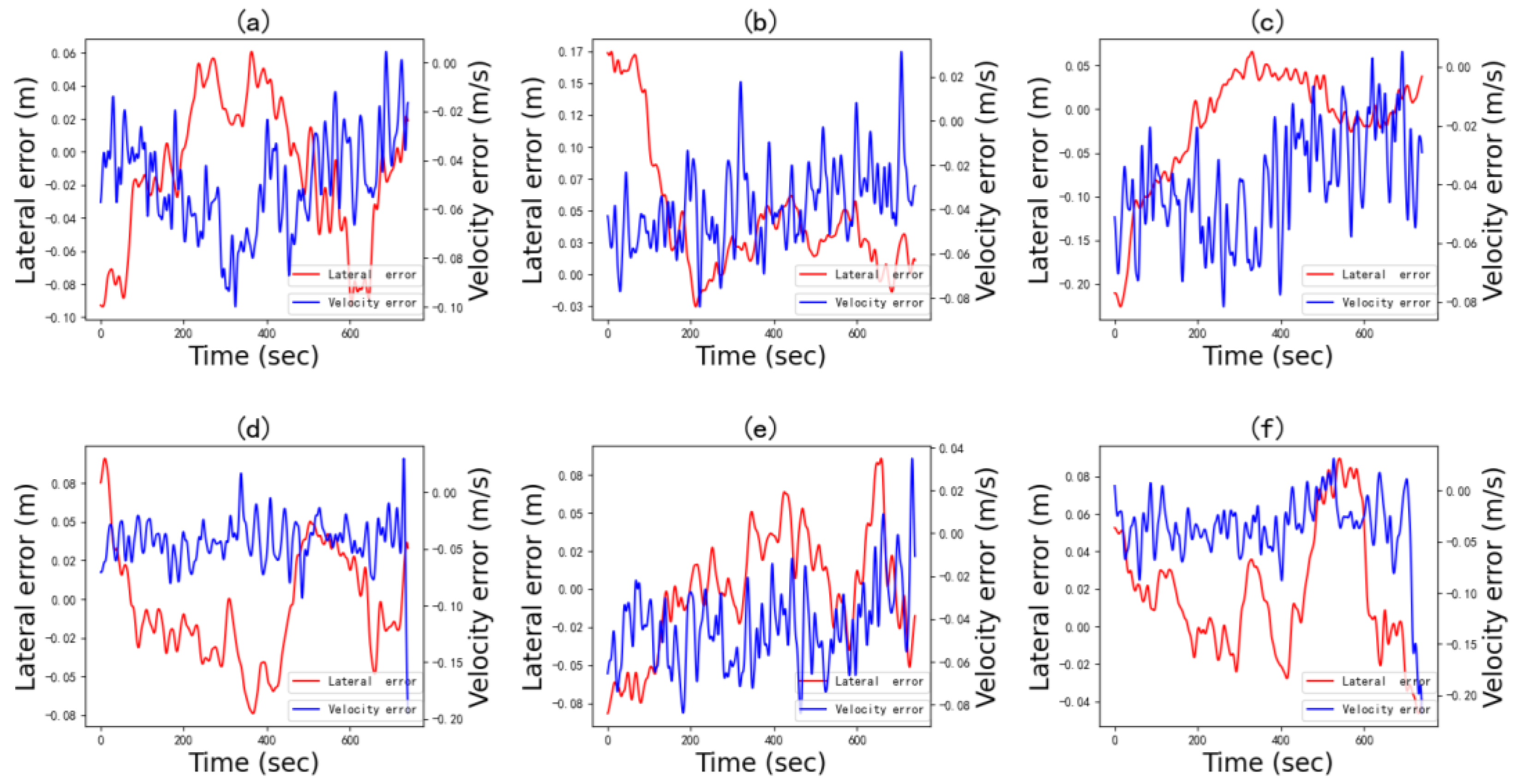
3. Results and Discussion
4. Conclusions
Author Contributions
Funding
Institutional Review Board Statement
Data Availability Statement
Conflicts of Interest
References
- Yin, X.; An, J.; Wang, Y.; Wang, Y.; Jin, C. Development and experiments of the autonomous driving system for high-clearance spraying machines. Trans. Chin. Soc. Agric. Eng. 2021, 37, 22–30. [Google Scholar]
- Liu, Z.; Zhang, Z.; Luo, X.; Wang, H.; Huang, P.; Zhang, J. Design of automatic navigation operation system for Lovol ZP9500 high clearance boom sprayer based on GNSS. Trans. Chin. Soc. Agric. Eng. 2018, 34, 15–21. [Google Scholar]
- Zhang, M.; Ji, Y.H.; Li, S.C.; Cao, R.; Xu, H.; Zhang, Z. Research Progress of Agricultural Machinery Navigation Technology. Trans. Chin. Soc. Agric. Mach. 2020, 51, 1–18. [Google Scholar]
- Roshanianfard, A.; Noguchi, N.; Okamoto, H.; Ishii, K. A review of autonomous agricultural vehicles (The experience of Hokkaido University). J. Terramech. 2020, 91, 155–183. [Google Scholar] [CrossRef]
- Ljungqvist, O.; Evestedt, N.; Axehill, D.; Cirillo, M.; Pettersson, H. A Path Planning and Path-following Control Framework for a General 2-trailer with a Car-like Tractor. J. Field Robot. 2019, 36, 1345–1377. [Google Scholar] [CrossRef]
- Chen, K.; Jie, Y.S.; Li, Y.M.; Liu, C.; Mo, J. Full Coverage Path Planning Method of Agricultural Machinery. Trans. Chin. Soc. Agric. Mach. 2022, 53, 17–26. [Google Scholar]
- Yang, Y.; Wen, X.; Ma, Q.L.; Zhang, G.; Cheng, S.; Qi, J.; Chen, Z.; Chen, L. Real time planning of the obstacle avoidance path of agricultural machinery in dynamic recognition areas based on Bezier curve. Trans. Chin. Soc. Agric. Eng. 2022, 38, 34–43. [Google Scholar]
- Zhou, J.; He, Y. Research Progress on Navigation Path Planning of Agricultural Machinery. Trans. Chin. Soc. Agric. Mach. 2021, 52, 1–14. [Google Scholar] [CrossRef]
- Wang, H.; Wang, G.M.; Luo, X.W.; Zhang, Z.G.; Gao, Y.; He, J.; Yue, B. Path tracking control method of agricultural machine navigation based on aiming pursuit model. Trans. Chin. Soc. Agric. Eng. 2019, 35, 11–19. [Google Scholar]
- Murillo, M.; Sanchez, G.; Deniz, N.; Genzelis, L. Improving path-tracking performance of an articulated tractor-trailer system using a non-linear kinematic model. Comput. Electron. Agric. 2022, 196, 106826. [Google Scholar] [CrossRef]
- Khalaji, A.K. PID-based target tracking control of a tractor-trailer mobile robot. Proc. Inst. Mech. Eng. Part C J. Mech. Eng. Sci. 2019, 233, 4776–4787. [Google Scholar] [CrossRef]
- Yang, Y.; Li, Y.; Wen, X.; Zhang, G.; Ma, Q.; Cheng, S.; Qi, J.; Xu, L.; Chen, L. An optimal goal point determination algorithm for automatic navigation of agricultural machinery: Improving the tracking accuracy of the Pure Pursuit algorithm. Comput. Electron. Agric. 2022, 194, 106760. [Google Scholar] [CrossRef]
- Soylu, S.; Çarman, K. Fuzzy logic based automatic slip control system for agricultural tractors. J. Terramech. 2021, 95, 25–32. [Google Scholar] [CrossRef]
- He, J.; Hu, L.; Wang, P.; Liu, Y.; Man, Z.; Tu, T.; Yang, L.; Li, Y.; Yi, Y.; Li, W.; et al. Path tracking control method and performance test based on agricultural machinery pose correction. Comput. Electron. Agric. 2022, 200, 107185. [Google Scholar] [CrossRef]
- Delavarpour, N.; Eshkabilov, S.; Bon, T.; Nowatzki, J.; Bajwa, S. The tractor-cart system controller with fuzzy logic rules. Appl. Sci. 2020, 10, 5223. [Google Scholar] [CrossRef]
- Meng, Q.K.; Chou, R.C.; Zhang, M.; Liu, G.; Zhang, Z.; Xiang, M. Navigation System of Agricultural Vehicle Based on Fuzzy Logic Controller with Improved Particle Swarm Optimization Algorithm. Trans. Chin. Soc. Agric. Eng. 2015, 46, 29–36. [Google Scholar]
- Manikandan, S.; Kaliyaperumal, G.; Hakak, S.; Gadekallu, T.R. Curve-Aware Model Predictive Control (C-MPC) Trajectory Tracking for Automated Guided Vehicle (AGV) over On-Road, In-Door, and Agricultural-Land. Sustainability 2022, 14, 12021. [Google Scholar] [CrossRef]
- Vatavuk, I.; Vasiljević, G.; Kovačić, Z. Task Space Model Predictive Control for Vineyard Spraying with a Mobile Manipulator. Agriculture 2022, 12, 381. [Google Scholar] [CrossRef]
- Li, Y.; He, D.; Ma, F.; Liu, P.; Liu, Y. MPC-based trajectory tracking control of unmanned underwater tracked bulldozer considering track slipping and motion smoothing. Ocean Eng. 2023, 279, 114449. [Google Scholar] [CrossRef]
- Sportelli, M.; Apolo-Apolo, O.E.; Fontanelli, M.; Frasconi, C.; Raffaelli, M.; Peruzzi, A.; Perez-Ruiz, M. Evaluation of YOLO Object Detectors for Weed Detection in Different Turfgrass Scenarios. Appl. Sci. 2023, 13, 8502. [Google Scholar] [CrossRef]
- Ajayi, O.G.; Ashi, J.; Guda, B. Performance evaluation of YOLO v5 model for automatic crop and weed classification on UAV images. Smart Agric. Technol. 2023, 5, 100231. [Google Scholar] [CrossRef]
- Wang, C.; Wu, X.; Zhang, Y.; Wang, W. Recognition and segmentation of maize seedlings in field based on dual attention semantic segmentation network. Trans. Chin. Soc. Agric. Eng. 2021, 37, 211–221. [Google Scholar]
- Selvaraj, M.G.; Vergara, A.; Ruiz, H.; Safari, N.; Elayabalan, S.; Ocimati, W.; Blomme, G. AI-powered banana diseases and pest detection. Plant Methods 2019, 15, 92. [Google Scholar] [CrossRef]
- Domingues, T.; Brandão, T.; Ferreira, J.C. Machine learning for detection and prediction of crop diseases and pests: A comprehensive survey. Agriculture 2022, 12, 1350. [Google Scholar] [CrossRef]
- Meshram, A.T.; Vanalkar, A.V.; Kalambe, K.B.; Badar, A.M. Pesticide spraying robot for precision agriculture: A categorical literature review and future trends. J. Field Robot. 2022, 39, 153–171. [Google Scholar] [CrossRef]
- Özlüoymak, Ö.B. Development and assessment of a novel camera-integrated spraying needle nozzle design for targeted micro-dose spraying in precision weed control. Comput. Electron. Agric. 2022, 199, 107134. [Google Scholar] [CrossRef]
- Blasco, J.; Aleixos, N.; Roger, J.M.; Rabatel, G.; Moltó, E. AE—Automation and emerging technologies: Robotic weed control using machine vision. Biosyst. Eng. 2002, 83, 149–157. [Google Scholar] [CrossRef]
- Bakker, T.; Bontsema, J.; Müller, J. Systematic design of an autonomous platform for robotic weeding. J. Terramech. 2010, 47, 63–73. [Google Scholar] [CrossRef]
- Raja, R.; Nguyen, T.T.; Vuong, V.L.; Slaughter, D.C.; Fennimore, S.A. RTD-SEPs: Real-time detection of stem emerging points and classification of crop-weed for robotic weed control in producing tomato. Biosyst. Eng. 2020, 195, 152–171. [Google Scholar] [CrossRef]
- Manyam, S.G.; Rathinam, S. On tightly bounding the dubins traveling salesman’s optimum. J. Dyn. Syst. Meas. Control 2018, 140, 71013. [Google Scholar] [CrossRef]
- Chen, Y.; He, Y. Development of agricultural machinery steering wheel angle measuring system based on GNSS attitude and motor encoder. Trans. Csae 2021, 37, 10–17. [Google Scholar]
- Wang, D.; He, D. Channel pruned YOLO V5s-based deep learning approach for rapid and accurate apple fruitlet detection before fruit thinning. Biosyst. Eng. 2021, 210, 271–281. [Google Scholar] [CrossRef]


| Technical Indicators | Value |
|---|---|
| Engine power (kW) | 15.4 |
| Length × width × height (m) | 4.1 × 2.2 × 2.54 |
| Spraying width (m) | 2 |
| Ground clearance (m) | 1.2 |
| Turning radius (m) | 3.5 |
| Tank volume (L) | 500 |
| Speed (km·h−1) | 0–5.6 |
| Autopilot accuracy (cm) | ±2.5 |
| Weed identification rate (%) | >80 |
Disclaimer/Publisher’s Note: The statements, opinions and data contained in all publications are solely those of the individual author(s) and contributor(s) and not of MDPI and/or the editor(s). MDPI and/or the editor(s) disclaim responsibility for any injury to people or property resulting from any ideas, methods, instructions or products referred to in the content. |
© 2023 by the authors. Licensee MDPI, Basel, Switzerland. This article is an open access article distributed under the terms and conditions of the Creative Commons Attribution (CC BY) license (https://creativecommons.org/licenses/by/4.0/).
Share and Cite
Yang, T.; Jin, C.; Ni, Y.; Liu, Z.; Chen, M. Path Planning and Control System Design of an Unmanned Weeding Robot. Agriculture 2023, 13, 2001. https://doi.org/10.3390/agriculture13102001
Yang T, Jin C, Ni Y, Liu Z, Chen M. Path Planning and Control System Design of an Unmanned Weeding Robot. Agriculture. 2023; 13(10):2001. https://doi.org/10.3390/agriculture13102001
Chicago/Turabian StyleYang, Tengxiang, Chengqian Jin, Youliang Ni, Zhen Liu, and Man Chen. 2023. "Path Planning and Control System Design of an Unmanned Weeding Robot" Agriculture 13, no. 10: 2001. https://doi.org/10.3390/agriculture13102001
APA StyleYang, T., Jin, C., Ni, Y., Liu, Z., & Chen, M. (2023). Path Planning and Control System Design of an Unmanned Weeding Robot. Agriculture, 13(10), 2001. https://doi.org/10.3390/agriculture13102001