Article

Extracting Tea Plantations from Multitemporal Sentinel-2 Images Based on Deep Learning Networks

1
School of Geographical Sciences, Nanjing University of Information Science and Technology, Nanjing 210044, China
2
School of Applied Meteorology, Nanjing University of Information Science and Technology, Nanjing 210044, China
3
Key Laboratory of Transportation Meteorology, China Meteorological Administration, Nanjing 210041, China
4
Jiangsu Institute of Meteorological Sciences, Nanjing 210041, China
5
Nanjing Joint Institute for Atmospheric Sciences, Nanjing 210041, China
*
Author to whom correspondence should be addressed.
Agriculture 2023, 13(1), 10; https://doi.org/10.3390/agriculture13010010
Submission received: 11 November 2022 / Revised: 10 December 2022 / Accepted: 19 December 2022 / Published: 21 December 2022
(This article belongs to the Section Digital Agriculture)

Abstract

:
Tea is a special economic crop that is widely distributed in tropical and subtropical areas. Timely and accurate access to the distribution of tea plantation areas is crucial for effective tea plantation supervision and sustainable agricultural development. Traditional methods for tea plantation extraction are highly dependent on feature engineering, which requires expensive human and material resources, and it is sometimes even difficult to achieve the expected results in terms of accuracy and robustness. To alleviate such problems, we took Xinchang County as the study area and proposed a method to extract tea plantations based on deep learning networks. Convolutional neural network (CNN) and recurrent neural network (RNN) modules were combined to build an R-CNN model that can automatically obtain both spatial and temporal information from multitemporal Sentinel-2 remote sensing images of tea plantations, and then the spatial distribution of tea plantations was predicted. To confirm the effectiveness of our method, support vector machine (SVM), random forest (RF), CNN, and RNN methods were used for comparative experiments. The results show that the R-CNN method has great potential in the tea plantation extraction task, with an F1 score and IoU of 0.885 and 0.793 on the test dataset, respectively. The overall classification accuracy and kappa coefficient for the whole region are 0.953 and 0.904, respectively, indicating that this method possesses higher extraction accuracy than the other four methods. In addition, we found that the distribution index of tea plantations in mountainous areas with gentle slopes is the highest in Xinchang County. This study can provide a reference basis for the fine mapping of tea plantation distributions.

1. Introduction

Tea is an evergreen woody plant whose leaves can produce a beverage that is known as one of the world’s three major drinks together with cocoa and coffee [1]. As an economically important crop, tea plays a significant role in promoting the prosperity of many developing countries [2]. Accounting for nearly 38% of the global total tea yield, China has the largest tea industry in the world, as it plants and produces tea in more than 20 provinces [3]. According to statistics, as one of the major provinces producing tea in China, Zhejiang Province produced approximately 177,200 tons of tea in 2020 [4], which accounted for a considerable proportion of the national tea yield. With the growing demand for tea, the area of tea plantations is also increasing. On one hand, tea can promote the development of the local economy, but on the other hand, it may cause some negative effects, such as the destruction of the ecological environment. At present, it is an urgent problem to implement correct supervision of tea plantations and effectively maintain a balance between the economic benefits brought by tea production and a series of adverse effects caused by the expansion of tea plantations. However, how to efficiently and accurately acquire the spatial distribution of tea plantations has always been a difficult problem in the process of fine and dynamic management of tea plantations. Therefore, the proposal of an effective method for extracting tea plantations is of great significance for monitoring the area of tea plantations and carrying out tea tree disaster alert work, thus improving tea production and quality. In addition, it can enhance the standardized management of tea plantations to boost garden greening configurations, conserve water, improve soil quality, raise biodiversity, and promote the sustainable development of the ecological environment.
Remote sensing is a technology that enables the detection of objects at a distance without contact. Given the advantages of prompt information acquisition and a wide observation range, remote sensing technology is widely used in resource census, land use planning, environmental monitoring, and so on [5,6,7,8]. With the rapid development of science and technology in recent years, the temporal, spatial, and spectral resolution of remote sensing satellite images has been continuously improved. A large number of studies have been conducted to use these images for the extraction of crop plantation areas [9,10,11,12], among which the most extensively used remote sensing images are derived from the Gaofen satellites of China, the Sentinel satellites within the European Copernicus program, and the Landsat satellites within the Landsat Project of the United States. With rich spectral, spatial, and temporal information, many crops can be classified, effectively avoiding interference by the phenomenon of “different body with the same spectrum” and “same body with different spectra” [13]. Consequently, remote sensing technology is conducive to monitoring the planting area of many kinds of crops quickly, accurately, and efficiently to provide a reference for planting area statistics, spatial distribution mapping, etc.
The traditional methods for extracting tea plantations include field measurements and statistics, which are inefficient and not timely and do not meet the needs of modern agricultural development. To alleviate such problems, several scholars have conducted a series of studies on the extraction of tea plantations using multispectral remote sensing images, such as Sentinel [14,15,16], Modis [17], and Landsat [17,18,19] images. In addition, the methods they used are mainly traditional machine learning algorithms, such as decision tree (DN) [14,17,20], support vector machine (SVM) [15,16,21,22], maximum likelihood (ML) [23,24], and random forest (RF) [16,19,20,23]. These algorithms have a single structure, simple rules, and fine classification performance in specific cases but require the manual construction of corresponding features derived from specific prior knowledge to train the model. Among these studies, the commonly used features include three types: spectral, texture, and terrain features. Fine results can be achieved by using one or more of these types of features, but more types of features generally lead to better results [15,17,23]. Nevertheless, this type of method requires much expertise and a large workload for feature engineering. In addition, the features that can be used are very limited if considering computational efficiency at the same time, and the selected features can hardly represent the characteristics of tea plantations completely or summarize the differences between tea plantations and other categories. Accordingly, the generalizability is relatively poor [25], which means that the resulting model usually has difficulty achieving the expected classification outcomes in other study areas.
In recent years, deep learning has gradually emerged. Owing to the ability to automatically acquire deep features of the data effectively, it has been widely used in many fields. Compared with traditional machine learning algorithms, deep learning networks can achieve stronger robustness and higher extraction efficiency without manual features [26]. CNNs are deep learning algorithms with local connection and weight-sharing characteristics. Due to their advantages in spatial feature processing, CNNs have played an important role in various remote sensing tasks, including scene recognition [27], land use classification [28], super resolution [29], target detection [30], and data reconstruction [31]. Likewise, some scholars have carried out research on the extraction of tea plantations by CNN methods [26,32,33,34,35]. Tea trees are usually cultivated by ridge planting and are arranged in strips, so tea plantations have specific spatial characteristics in remote sensing images. In addition, owing to the existence of the phenological period, the growth of tea trees shows periodic changes on an annual scale, which makes the characteristics of tea plantations in different periods of a year have specific change rules. However, most of the current studies only consider either the spatial or temporal characteristics of tea plantations in the images or only integrate the classification results of the two through image postprocessing technology [26,33,34,35]. There is still a lack of an end-to-end method to extract tea plantations that comprehensively considers the spatiotemporal features.
Recurrent neural networks (RNNs) are algorithms that can process data with time-series characteristics and prominently contribute to fields such as machine translation, speech recognition, and video processing. Moreover, some studies have demonstrated their greater potential in crop classification of time-series remote sensing data [10,11,36,37]. However, the input data of RNN-type models usually need to be processed into one-dimensional forms, resulting in ineffective use of spatial information. In view of the superiority of CNNs and RNNs in extracting spatial and temporal information, respectively, the purpose of our study is to construct an R-CNN method to extract the distribution of tea plantations in Xinchang County on multitemporal Sentinel-2 images and evaluate its performance. Thereafter, we attained a fine spatial distribution of tea plantations and then analyzed the distribution characteristics of tea plantations with changes in elevation and slope.
The remainder of the paper is structured as follows: Section 2 introduces the study area and data, Section 3 describes the methods proposed for classifying tea plantations, Section 4 analyzes the experimental results, Section 5 discusses the research, and Section 6 provides the main conclusion of the article.

2. Study Area and Data Acquisitions

2.1. Study Area

Xinchang County (Figure 1) is situated in Zhejiang Province, China, with 12 townships under its jurisdiction. Its geographical location lies between 120°41′–121°13′ E and 29°13′–29°33′ N, spanning approximately 52.3 km from east to west and 36.9 km from north to south. Known as “eight mountains, half water and half fields”, Xinchang County covers an area of approximately 1213 square kilometers, most of which is dominated by dry land and forests. It has a subtropical monsoon climate, with hot and rainy summers, mild and humid winters, and rain and heat over the same period. The average annual temperature, precipitation, and sunshine hours in Xinchang County are 16.6 °C, 1500 mm, and 1900 h, respectively, which are suitable for growing tea trees [38]. Having a well-developed tea economy, Xinchang County is the hometown of Chinese tea and is named the national tea standardization demonstration county and one of the top-ten key tea-producing counties in China.

2.2. Research Data

In this study, Sentinel-2 images were used as remote sensing data from the ESA Copernicus Data Centre (https://scihub.copernicus.eu (accessed on 30 March 2022)). Sentinel-2 is a high-resolution satellite with a multispectral imager (MSI), and it mainly contributes to land use change detection, vegetation growth monitoring, and emergency disaster relief [39,40,41,42]. The revisit period of Sentinel-2 can reach 5 days under the cooperation of the A and B binaries. Each Sentinel-2 image has a width of 290 km and contains 13 spectral bands, as shown in Table 1.
The ancillary data for analyzing the distribution of the predicted tea plantations are digital elevation model (DEM) data produced by the Advanced Land Observing Satellite (ALOS) observations from the Alaska Satellite Data Centre (https://search.asf.alaska.edu (accessed on 16 March 2022)). Its spatial resolution is 12.5 m.

3. Materials and Methods

3.1. Data Preprocessing

Influenced by phenology and human management, the characteristics of tea plantations vary in different periods. In Zhejiang Province, from approximately the end of February to March, tea trees are in the budding stage; from approximately March to April, tea trees are artificially pruned after the harvest; from approximately June to September, the pruned tea trees grow again and gradually reach the peak growth stage; from approximately October to November, with the gradual drop in temperature, tea trees enter a period of slow growth; and from approximately December to the next year in early February, tea trees enter the dormancy period as the temperature plummets further [14,43]. Thus, we obtained low-cloud volume Sentinel-2 L1C images (atmospheric apparent reflectance products after ortho correction and geometric fine correction) from the Copernicus Data Center of ESA on five dates—23 February, 13 May, 22 July, 9 November, and 24 December 2020. The Sen2Cor plug-in in ESA Snap software was used for atmospheric correction of the images to generate the L2A product image. Then, the image data were processed through band resampling, format conversion, layer stacking, and image mosaic processing. The multitemporal Sentinel-2 remote sensing image of the study area was obtained by clipping the processed image according to the vector file of the study area.
Based on the preprocessed Sentinel-2 images, 3 atmospheric bands (B1, B9, and B10) were removed, and finally, the reflectivity of 10 spectral bands (B2, B3, B4, B5, B6, B7, B8, B8A, B11, and B12) were used as the initial input features. In addition, we calculated six frequently used vegetation indices for input feature combination experiments, including normalized difference vegetation index (NDVI) [44], modified normalized difference vegetation index (MNDVI) [21], enhanced vegetation index (EVI) [45], normalized difference vegetation index red-edge 1 (NDVIre1), normalized difference vegetation index red-edge 2 (NDVIre2), and normalized difference vegetation index red-edge 3 (NDVIre3) [46]. The calculation formulas for the vegetation indices are shown in Table 2 below.
Meanwhile, we measured the effect of different input features on the performance of the R-CNN model by designing five combination schemes as the initial input features: (1) common bands (B2, B3, B4, and B8); (2) common bands and red edge vegetation bands (B2, B3, B4, B5, B6, B7, and B8); (3) common bands and SWIR bands (B2, B3, B4, B8, B11, and B12); (4) all spectral bands; and (5) all spectral bands and vegetation indices.
By referring to the VHR Google Earth image of the corresponding period, we selected 278,528 pixels from Sentinel 2 in the study area as sample sets, comprising 75,147 tea plantation pixels and 203,381 pixels of other ground objects. According to the principle that the data in different sets are independent of each other and the distribution of each class in all sets is similar [36], they were randomly divided into three datasets: training dataset, validation dataset, and test dataset, with a division ratio of 3:1:1. The training dataset was used to train the classification model, the validation dataset was used to select the best parameters, and the test dataset was used to evaluate the accuracy of the classification model. Each dataset contained several groups of data that consisted of an image and a corresponding label.

3.2. R-CNN Method for Tea Plantation Extraction

CNN is a classical deep learning algorithm. The convolutional layers are the core part of the CNN, which uses convolutional kernels to operate the input features and calculates the output features x o u t through the activation function [47]. The calculation formula is as follows:
x o u t = f w x i n + b i a s
In Equation (1), w is the weight vector, x i n is the input features, b i a s is the offset vector, and f is the activation function. Due to their powerful ability to extract spatial features, CNNs have made great achievements in image semantic segmentation. Presently, there are numerous widely used semantic segmentation models, including FCN [48], SegNet [49], PSPNet [50], UNet [51], and DeepLabv3 [52]. Among them, the UNet model has a simple structure, multiscale feature extraction capability, and excellent extraction results with only a small number of samples. UNet is mainly composed of two parts: the contracting path is mainly used to obtain context information and extract features, and the expansion path is mainly used for precise positioning, which means mapping concentrated features to corresponding positions and then outputting predicted results. In addition, each level in the contracting path uses a skip connection to concatenate the features with those at the same level in the expansion path, which fuses both the shallow-level features and deep-level features and effectively combines local information and global information [53]. However, the original UNet model is limited to the segmentation of a single time-stage image and cannot obtain the temporal information in multitemporal images.
Unlike CNNs, RNNs are structures that focus on processing time-series information, including long short-term memory (LSTM) [54] network and gated recurrent unit (GRU) [55] network, which are widely used. Compared with LSTM, GRU has the superiority of fewer parameters and being applicable to small datasets. The GRU network has inputs and outputs similar to those of an ordinary RNN network in general. The inputs comprise the input value x t at time t and the state h t 1 at time t 1 , and the outputs consist of the output value y t and the state h t at time t . Update and reset gates are two unique characteristics of GRU. The update gate decides whether to replace the hidden state at the previous time with a new hidden state. First, at time t , the update gate z t is calculated:
z t = σ W z x · x t + W z h · h t 1 + b z
The reset gate decides whether to forget the hidden state at the previous time. Then, the reset gate r t at time t is calculated:
r t = σ W r x · x t + W r h · h t 1 + b r
Additionally, based on the reset gate, the new hidden state h t is calculated as a candidate, and the calculation formula is as follows:
h t = t a n h W h x · x t + W h h · ( r t h t 1 + b h )
Eventually, the update gate updates the hidden state and obtains the final output h t . The calculation formula is as follows:
h t = z t h t 1 + 1 z t h t
In Equations (2)–(5), σ is the logical sigmoid activation function, W z x , W z h , W r x , W r h , W h x , and W h h are the weight matrices, b z , b r , and b h are the offset vectors, t a n h is the hyperbolic tangent activation function, and is the Hadamard product.
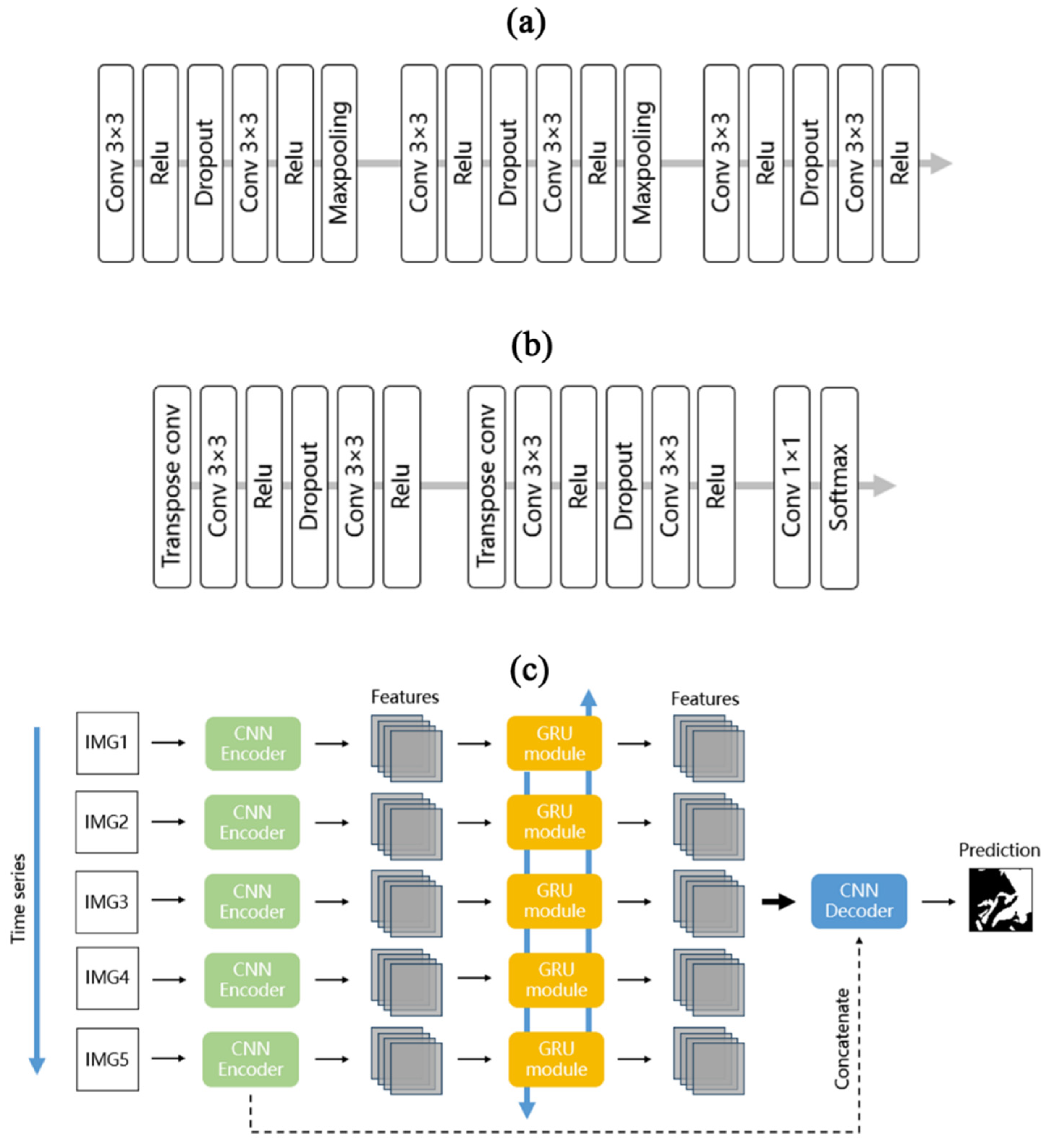
We constructed an R-CNN model based on the UNet structure and GRU modules, as shown in Figure 2. The model is mainly composed of three parts: CNN encoders, GRU modules, and a CNN decoder. First, each batch of data is input into the model through six 3 × 3 convolutional layers (with a stride of 1, the “same” padding, and a ReLU activation function) and two 2 × 2 maxpooling layers. To effectively enhance robustness and prevent the model from overfitting, a dropout layer is added after the first convolutional layer of each level. Second, the extracted feature vectors of spatial information are fed to the GRU modules in the time series, and the hidden state sequence is calculated by the GRU network. Note that we use a bidirectional GRU network here that can integrate information from both forward and backward states. In addition, four 3 × 3 convolutional layers and two 2 × 2 transposed convolutional layers are built to map the features with the same spatial resolution size as the input data. Meanwhile, the skip connection in the original UNet model is retained in our model. Finally, a 1 × 1 convolutional layer and softmax activation function are used to output the predicted results.

3.3. Other Methods for Comparison

We compared the tea plantation extraction results from our proposed method with those from the following methods:
(1)
RF [56] classification method: The RF classification algorithm is a traditional machine learning method developed from the decision tree (DT) algorithm, which has the benefits of high training speed and a small possibility of overfitting. It randomly extracts some data from the initial samples and reassembles them into sample subsets, then generates multiple decision trees to train the sample subsets, and finally integrates the voting results of each decision tree to determine the final predicted result of the classification model.
(2)
SVM [57] classification method: The SVM classification algorithm is a traditional machine learning method with the advantages of a simple structure and insensitivity to outliers. It maps the sample data into a high-dimensional space and solves for an optimal hyperplane in which to partition the data so that the data closest to the hyperplane on each side are as far away from the hyperplane as possible, based on which the sample data can be classified and predicted.
(3)
CNN classification method: The CNN classification model in the comparison experiments is built based on the original UNet structure, i.e., removing the GRU module from the R-CNN model and using only the CNN encoder and CNN decoder.
(4)
RNN classification method: The bidirectional GRU module is used to construct the RNN classification model in the comparison experiments.

3.4. Experimental Settings

In this experiment, we used the PyTorch framework to build the deep learning model on a Windows 10 system, an AMD Ryzen 7 4800H CPU, and an NVIDIA GeForce RTX 2060 GPU with 6 GB memory. In the training stage, the image data were first normalized by standard deviation and split into patches, and the image patch sets were fed into the model for feature extraction and feature mapping to obtain preliminary prediction results. Next, a loss function was used to calculate the error between the predicted result and the ground truth, and an adaptive moment estimation (Adam) optimizer was used to perform backpropagation iterations to dynamically adjust the parameters and learning rate of the model. Moreover, early stopping was set to avoid overfitting on the training dataset, which means that if the loss values on the validation dataset do not improve in 10 consecutive epochs of training, the model training will be terminated early. Ultimately, the trained model that had the smallest loss value on the validation dataset was selected as the optimal model. The specific hyperparameter settings before training are shown in Table 3.

3.5. Evaluation Indicators

The tea plantation extraction task in this study is a semantic segmentation binary classification task, so we introduced the evaluation metrics F1 score and IoU, which are commonly used in semantic segmentation to evaluate the predicted results on the test dataset. The F1 score reflects the precision and recall of the classification results in a comprehensive manner, and the intersection over union (IoU) describes the overlap rate between the classification results and the ground truth. The final score of each evaluation indicator is derived from tenfold cross-validation. The formulas for the evaluation indicators are
F 1 = 2 × p × r p + r
IoU = S p r e d S t r u t h S p r e d S t r u t h
where p is the precision, r is the recall, S p r e d S t r u t h is the intersection of the predicted and true areas for tea plantations, and S p r e d S t r u t h is the union of the predicted and true areas for tea plantations.
In addition, to evaluate the predicted spatial distribution of tea plantations in the study area from each extraction method, we combined the field survey results and visual interpretation of the randomly generated points on Google Earth images to select a total of 2166 verification points in the study area, including 920 points for tea plantations and 1246 points for other ground objects. Then, confusion matrices were created for the classification results of each method. Although the confusion matrices can visually represent the number of samples that are correctly or incorrectly predicted in each class, they cannot directly provide a detailed evaluation. Consequently, the following evaluation metrics were calculated based on the confusion matrix, including the overall accuracy (OA), commission error (CE), omission error (OE), and kappa coefficient. Overall accuracy refers to the proportion of the total number of verification points correctly classified; commission error represents the proportion of verification points predicted to be in a class that is actually not in that class; omission error refers to the proportion of verification points actually in a class that are predicted not to be in that class; and the kappa coefficient represents the proportion of improvement in the prediction of the classification method compared to completely random classification:
O A = T P + T N T P + T N + F P + F N
C E = F P T P + F P
O E = F N T P + F N
K a p p a = O A p e 1 p e
p e = T P + F N T P + F P + F P + T N T N + F N T P + F N + F P + T N 2
In Equations (8)–(12), T P is the number of correctly classified tea plantation points, F N is the number of incorrectly classified tea plantation points, T N is the number of correctly classified other ground object points, and F P is the number of incorrectly classified other ground object points.
Furthermore, The distribution index [58] is applied to describe the relationship between the spatial distribution of tea plantations and topographical factors such as elevation and slope. Its calculation formula is as follows:
D = S S k × S i k S i
In Equation (13), D is the distribution index, S is the total area of the whole region, S k is the area of a specific grade of topographical factor k in the whole region, S i k is the area of class i , which is at a specific grade of topographical factor k in the whole region, S i is the area of class i in the whole region.

4. Results

4.1. Evaluation of Different Input Features

In the experiment, the models were trained and tested by five feature combination schemes on the datasets which have been described in the previous section. By taking the ground truth maps as references, the F1 score and IoU were calculated to evaluate the performance of the models trained by different input features. The higher their values are, the better the corresponding model performs. Table 4 illustrates the results of the above experiment.
We found that as the number of bands increases, the performance of the model improves, with the F1 score increasing from 0.774 to 0.885 and the IoU increasing from 0.631 to 0.793. The addition of the red-edge band and the shortwave infrared band enabled the model to achieve better performance [59,60], which implies that they play notable roles in tea plantation extraction. In addition, we found that adding vegetation indices to the initial input features barely affected the performance of the model, indicating that the R-CNN model can automatically learn the combinatorial relationships among different input features without the need for manual feature construction, which is similar to the findings of previous studies [61,62]. Therefore, in order to balance computational efficiency and extraction accuracy, all spectral bands were used as input features for the model in the following study.

4.2. Evaluation of Different Models

To demonstrate the superiority of the R-CNN method, we compared its performance with that of the other four methods in the tea plantation extraction task from a quantitative perspective by training and testing each model on the datasets, with the F1 score and IoU as evaluation metrics.
From the evaluation results for the five methods in Table 5, the R-CNN model achieved the best performance, with 0.03–0.111 higher F1 scores than the other models and 0.046–0.161 higher IoU values than the other models. Therefore, we tentatively concluded that the R-CNN method has the best performance in the tea plantation extraction task compared to the other four methods.
Furthermore, visualization of the prediction results can help better reflect the performance of each model. Therefore, several predicted maps of the five models and their ground truth on the test dataset are displayed in Figure 3. Since it is difficult to identify tea plantations directly on the Sentinel-2 images by the naked eye, the VHR images that we used to make ground truth maps are displayed as a reference instead. According to the figures, the predicted results of the SVM, RF, and RNN methods have more pepper noise and poorer edge continuity, while the predicted results of the CNN and R-CNN methods have smoother edges and less noise. This is because the former methods do not consider the spatial relationship among different image pixels in the classification process and predict each pixel value independently, while the latter methods consider spatial information. In addition, several forests and cultivated lands were misclassified as tea plantations in the extraction results of the SVM, RF, and CNN methods. This is probably because these three methods are less capable of processing temporal information and thus have poorer ability in distinguishing the phenological information of tea trees from other vegetation. Overall, the extraction results of the R-CNN method are the most consistent with the ground truth. Nevertheless, the R-CNN method automatically regards some tea plantations with small areas as noise and removes them or smooths some small objects, such as roads inside tea plantations, and classifies them as tea plantations, which is one of the main sources of error.

4.3. Spatial Distribution of Tea Plantations in Xinchang County

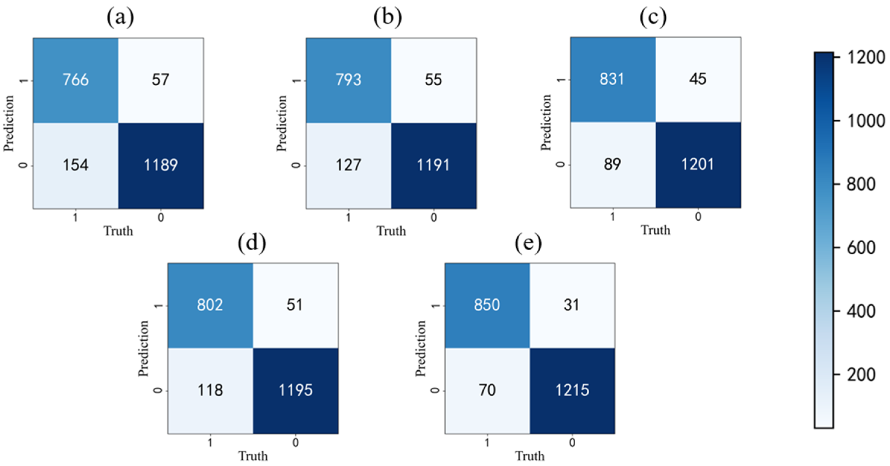
To attain the spatial distribution of tea plantations in Xinchang County, we segmented the images of the study area into small patches and input them into each model that had completed training to obtain the prediction results. Then, we put the small patches together in light of the corresponding geographical locations and finally obtained the spatial distribution map of tea plantations. The predicted results were quantitatively evaluated by the sample points derived from field work and visual interpretation. The confusion matrices and performance assessment are displayed in Figure 4 and Table 6, respectively.
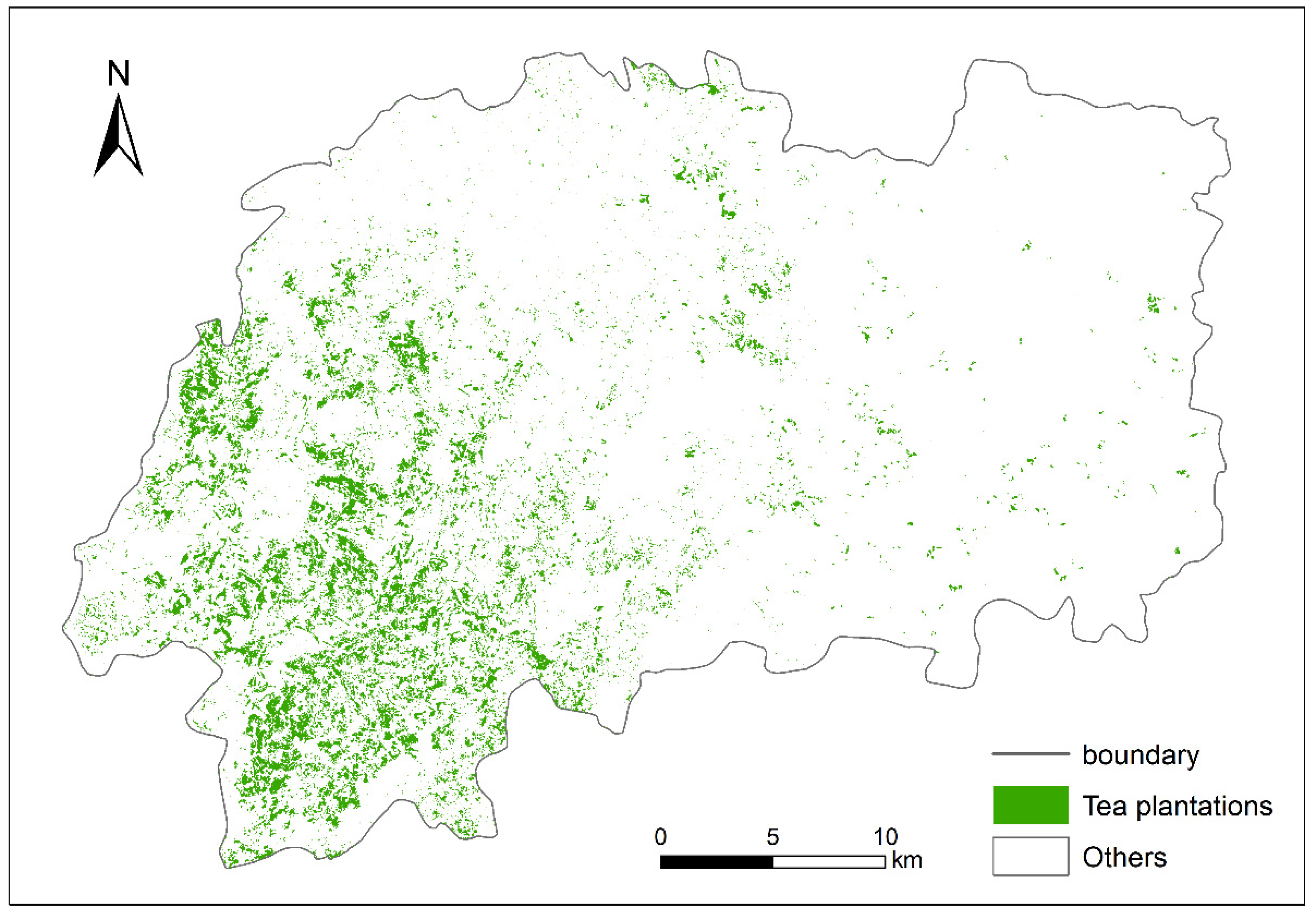
As Table 6 shows, the R-CNN method obtains the best classification performance. The commission error rate of tea plantations in the predicted results is 4.9%, the omission error rate of tea plantations is 6.3%, the overall accuracy is 95.3%, and the kappa coefficient is 0.904. The spatial distribution of tea plantations predicted by the R-CNN method is shown in Figure 5. We compared the sample points that were not correctly classified to the corresponding geographic locations on the VHR images and found that the commission error mainly occurs at the junction between tea plantations and other ground objects, while the omission error is mainly concentrated at the tea plantations with small areas. The limitations of the image spatial resolution and the mix of tea trees with other ground objects lead to the above situation to some extent. According to the Statistical Yearbook of Zhejiang Province [4], the area of tea plantations in Xinchang County in 2020 was approximately 8004 hectares. The total area of tea plantations extracted in this study is 8453 hectares, with a relative error of less than 10%, which is within a reasonable range. The existence of error is mainly related to the statistical survey method, complexity of the terrain, and limitations of the model itself.
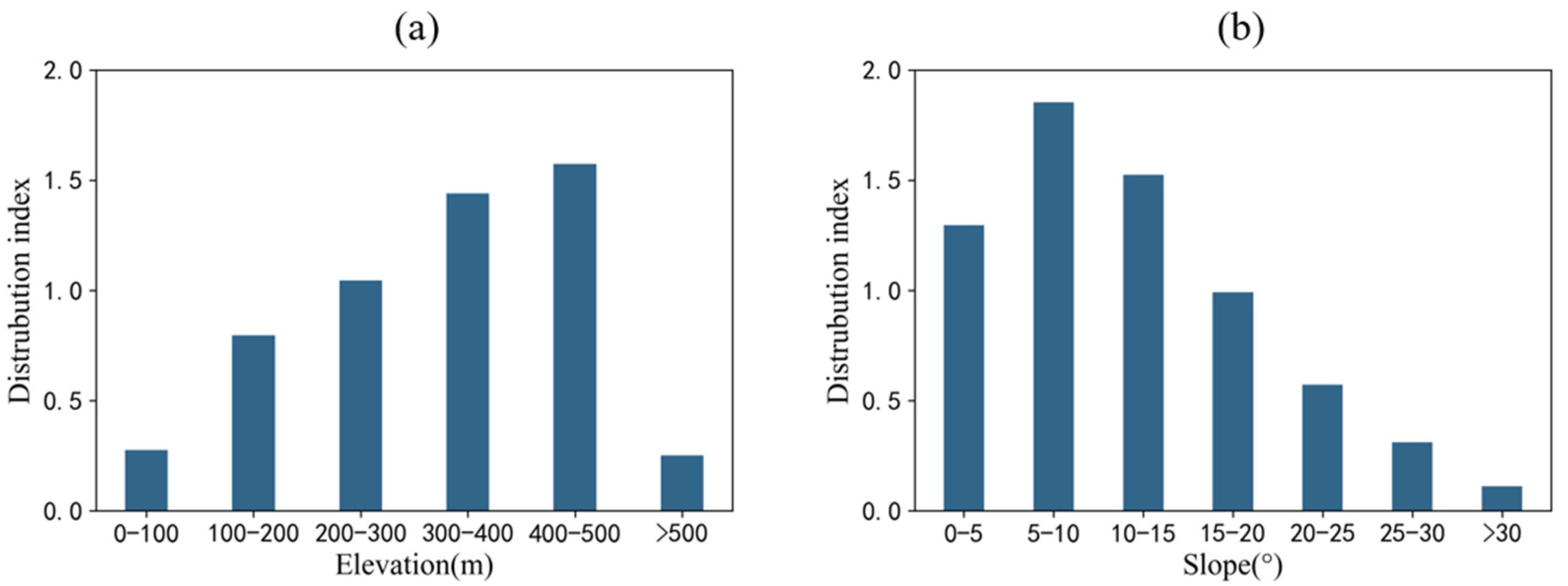
For further research on the spatial distribution characteristics of tea plantations in Xinchang County, considering topographic factors, we analyzed the tea plantations extracted from this study with DEM data. The distribution index is used to reflect the distribution characteristics of tea plantations at different altitudes and slopes. The elevation and slope intervals are set to 100 m and 5°, respectively. As shown in Figure 6a, the distribution index of tea plantations in Xinchang County shows a trend of increasing first and then decreasing in altitude. This is because the mountainous areas at certain altitudes have abundant rainfall, high air humidity, many clouds, and fog, which are conducive to the growth of tea trees. Moreover, according to Figure 6b, the distribution index of tea plantations achieves high values in the 5°–10° and 10°–15° ranges, which is related to the topographical conditions suitable for the growth of tea plantations. In general, the higher the slope inclination is, the thinner the soil layer. Thus, it has a poor ability to prevent water and fertility in soil from running off, which is adverse to the growth of tea trees.

5. Discussion

In this work, we used an end-to-end R-CNN method that combines CNN modules and RNN modules to extract tea plantations from multitemporal Sentinel-2 images. Recently, most of the relevant studies focus on using traditional machine learning methods or deep learning methods based on mono-temporal high-resolution images to extract tea plantations. The former relies heavily on the construction of manual features, which usually require considerable manpower, but it is sometimes still difficult to achieve the desired results. Although the latter achieves automation to some degree, it fails to effectively use the multispectral information and time-dimensional phenological information of the tea plantations in remote sensing images, resulting in numerous misclassified pixels between the tea plantations and other ground objects. In contrast, the method in our research has the following advantages: (1) It can automatically extract features from the original data without manually building additional features as the input data of the model, which helps reduce the amount of manpower. (2) In the feature extraction stage, it synthetically uses multispectral and spatiotemporal information to extract more comprehensive and robust features. (3) It is an end-to-end method for classification, and because the overall process complexity is low, it has high practicality. Our experimental results show that deep learning algorithms can markedly reduce misclassification [63,64], and CNNs that can effectively use spatial information and RNNs that can effectively use temporal information have complementary characteristics in tea plantation extraction. The R-CNN method obtains higher elevation scores in classifying tea plantations than the CNN method and RNN method, as well as traditional machine learning methods. Previous studies have successfully applied similar methods to land use classification [65,66], but few studies have applied them to tea plantation extraction, especially in an end-to-end way.
The extraction of tea plantations is still in the exploratory stage, and there are some limitations in this study. First, the experiments were conducted on a small dataset, and the model was constructed with a few layers and a simple structure to prevent overfitting. Although deep learning models commonly have better generalization capabilities than many traditional machine learning methods, the performance of the models is still influenced by the temporal and spatial coverage of the training datasets and the complexity of the models themselves. Therefore, when conducting province-wide or nationwide tea plantation extraction in the future, increasing the model complexity, as well as conducting data collection for multiple locations to increase the number and diversity of samples, can be considered to improve the generalization ability of models. In addition, the spatial resolution of the images used in this study is 10 m, which results in some tea plantations with small areas and the boundaries of the tea plantations forming mixed pixels with other ground objects in the image, leading to the misclassification of tea plantations in the predicted results. The use of multitemporal multispectral images with higher spatial resolution will be considered in the future to improve the accuracy of tea plantation extraction results and thereby provide technical support for the development of the tea industry.

6. Conclusions

In this paper, we explored the potential application of the R-CNN model in tea plantation extraction based on multitemporal and multispectral remote sensing images. This model transmits the multispectral image data to the CNN encoder to extract spatial features and then uses the GRU modules to further obtain the temporal information. After that, features of different scales are aggregated into the CNN decoder for the classification of tea plantations. Eventually, we evaluated the performance of the classification results and compared them with those of CNN, RNN, and two traditional machine learning methods that are widely used in classification tasks. We concluded that the R-CNN model that integrates spatiotemporal features achieves excellent extraction results from Sentinel-2 images, since it can not only effectively distinguish tea plantations from other ground objects with similar spectral characteristics but also reduce the pepper noise in the predicted results and increase edge smoothing. It achieved the highest overall accuracy and kappa coefficient of 0.953 and 0.904, respectively, in extracting the spatial distribution of tea plantations in Xinchang County. Furthermore, the predicted results of tea plantations from our method can contribute to the detection of annual area changes in tea plantations and the prediction of tea yield.

Author Contributions

Conceptualization, Z.Y., X.Z. and X.Q.; methodology, Z.Y.; software, Z.Y.; validation, Z.Y., X.Z. and Y.Z.; formal analysis, Z.Y.; investigation, X.Z.; resources, Z.Y.; data curation, Z.Y.; writing—original draft preparation, Z.Y.; writing—review and editing, Z.Y., X.Z., Y.Z. and X.Q.; visualization, Z.Y.; supervision, X.Z.; project administration, X.Z. and Y.Z.; funding acquisition, X.Z. and Y.Z. All authors have read and agreed to the published version of the manuscript.

Funding

This research was funded by the National Natural Science Foundation of China, grant numbers 41805049 and 42075118.

Institutional Review Board Statement

Not applicable.

Data Availability Statement

The data presented in this study are available on request from the corresponding author. The data are not publicly available due to the privacy policy of the authors’ institution.

Acknowledgments

Funding from the National Natural Science Foundation of China (41805049 and 42075118) is gratefully acknowledged. We also thank the editors and reviewers for their comments to improve our manuscript.

Conflicts of Interest

The authors declare no conflict of interest.

References

  1. Xiao, Z.; Huang, X.; Meng, H.; Zhao, Y. Spatial structure and evolution of tea production in China from 2009 to 2014. Geogr. Res. 2017, 36, 109–120. [Google Scholar]
  2. Chen, L.; Zhou, Z. Variations of main quality components of tea genetic resources [Camellia sinensis (L.) O. Kuntze] preserved in the China National Germplasm Tea Repository. Plant Foods Hum. Nutr. 2005, 60, 31–35. [Google Scholar] [CrossRef] [PubMed]
  3. Su, S.; Wan, C.; Li, J.; Jin, X.; Pi, J.; Zhang, Q.; Weng, M. Economic benefit and ecological cost of enlarging tea cultivation in subtropical China: Characterizing the trade-off for policy implications. Land Use Policy 2017, 66, 183–195. [Google Scholar] [CrossRef]
  4. Zhu, Y.; Zhang, X. Zhe Jiang Stastical Yearbook, 3rd ed.; China Statistics Publishing House: Beijing, China, 2021. [Google Scholar]
  5. Brezonik, P.L.; Olmanson, L.G.; Bauer, M.E.; Kloiber, S.M. Measuring water clarity and quality in minnesota lakes and rivers: A census-based approach using remote-sensing techniques. Cura Rep. 2007, 37, 3–313. [Google Scholar]
  6. Enoguanbhor, E.C.; Gollnow, F.; Nielsen, J.O.; Lakes, T.; Walker, B.B. Land cover change in the Abuja City-Region, Nigeria: Integrating GIS and remotely sensed data to support land use planning. Sustainability 2019, 11, 1313. [Google Scholar] [CrossRef] [Green Version]
  7. Vibhute, A.D.; Gawali, B.W. Analysis and modeling of agricultural land use using remote sensing and geographic information system: A review. Int. J. Eng. Res. Appl. 2013, 3, 81–91. [Google Scholar]
  8. Li, J.; Pei, Y.; Zhao, S.; Xiao, R.; Sang, X.; Zhang, C. A review of remote sensing for environmental monitoring in China. Remote Sens. 2020, 12, 1130. [Google Scholar] [CrossRef] [Green Version]
  9. Li, Z.; Chen, G.; Zhang, T. A CNN-transformer hybrid approach for crop classification using multitemporal multisensor images. IEEE J. Sel. Top. Appl. Earth Obs. Remote Sens. 2020, 13, 847–858. [Google Scholar] [CrossRef]
  10. Zhao, H.; Chen, Z.; Jiang, H.; Jing, W.; Sun, L.; Feng, M. Evaluation of three deep learning models for early crop classification using sentinel-1A imagery time series—A case study in Zhanjiang, China. Remote Sens. 2019, 11, 2673. [Google Scholar] [CrossRef] [Green Version]
  11. Zhong, L.; Hu, L.; Zhou, H. Deep learning based multi-temporal crop classification. Remote Sens. Environ. 2019, 221, 430–443. [Google Scholar] [CrossRef]
  12. Xu, J.; Yang, J.; Xiong, X.; Li, H.; Huang, J.; Ting, K.; Ying, Y.; Lin, T. Towards interpreting multi-temporal deep learning models in crop mapping. Remote Sens. Environ. 2021, 264, 112599. [Google Scholar] [CrossRef]
  13. Xie, Y.; Feng, D.; Shen, X.; Liu, Y.; Zhu, J.; Hussain, T.; Baik, S.W. Clustering Feature Constraint Multiscale Attention Network for Shadow Extraction From Remote Sensing Images. IEEE Trans. Geosci. Remote Sens. 2022, 60, 4705414. [Google Scholar] [CrossRef]
  14. Zhao, X.; Wang, P.; Jin, L.; Tan, B.; Zhao, X.; Liu, D. The application of spectral characteristics of time series Sentinel-2A images in tea land extraction. Sci. Surv. Mapp. 2020, 45, 80–88. [Google Scholar]
  15. Xiong, H.; Zhou, X.; Wang, X.; Cui, Y. Mapping the spatial distribution of tea plantations with 10 m resolution in Fujian province using Google Earth Engine. J. Geoinf. Sci. 2021, 23, 1325–1337. [Google Scholar]
  16. Chen, P.; Zhao, C.; Duan, D.; Wang, F. Extracting tea plantations in complex landscapes using Sentinel-2 imagery and machine learning algorithms. Community Ecol. 2022, 23, 163–172. [Google Scholar] [CrossRef]
  17. Ma, C.; Yang, F.; Wang, X. Extracting tea plantations in southern hilly and mountainous region based on mesoscale spectrum and temporal phenological features. Remote Sens. Land Resour. 2019, 31, 141–148. [Google Scholar] [CrossRef]
  18. Xu, W.; Huang, S.; Wu, C.; Xiong, Y.; Wang, L.; Lu, N.; Kou, W. The pruning phenological phase-based method for extracting tea plantations by field hyperspectral data and Landsat time series imagery. Geocarto Int. 2022, 37, 2116–2136. [Google Scholar] [CrossRef]
  19. Wang, B.; He, B.; Lin, N.; Wang, W.; Li, T. Tea plantation remote sensing extraction based on random forest feature selection. J. Jilin Univ. 2022, 52, 1719–1732. [Google Scholar]
  20. Huang, S.; Xu, W.; Xiong, Y.; Wu, C.; Dai, F.; Xu, H.; Wang, L.; Kou, W. Combining Textures and Spatial Features to Extract Tea Plantations Based on Object-Oriented Method by Using Multispectral Image. Spectrosc. Spectr. Anal. 2021, 41, 2565–2571. [Google Scholar]
  21. Dihkan, M.; Guneroglu, N.; Karsli, F.; Guneroglu, A. Remote sensing of tea plantations using an SVM classifier and pattern-based accuracy assessment technique. Int. J. Remote Sens. 2013, 34, 8549–8565. [Google Scholar] [CrossRef]
  22. Chen, Y.; Lin, J.; Yang, Y.; Wang, X. Extraction of tea plantation with high resolution Gaofen-2 image. In Proceedings of the 2019 8th International Conference on Agro-Geoinformatics (Agro-Geoinformatics), Istanbul, Turkey, 16–19 July 2019; pp. 1–6. [Google Scholar]
  23. Akar, Ö.; Güngör, O. Integrating multiple texture methods and NDVI to the Random Forest classification algorithm to detect tea and hazelnut plantation areas in northeast Turkey. Int. J. Remote Sens. 2015, 36, 442–464. [Google Scholar] [CrossRef]
  24. Xu, G. Research on Tea Garden Remote Sensing Extraction Based on Object-Oriented and Multi-Metadata Fusion. Master’s Thesis, Shaanxi Normal University, Xi’an, China, 2016. [Google Scholar]
  25. Yao, J.; Wu, J.; Yang, Y.; Shi, Z. Segmentation in multi-spectral remote sensing images using the fully convolutional neural network. J. Image Graph. 2020, 25, 180–192. [Google Scholar]
  26. Jamil, A.; Bayram, B. Automatic discriminative feature extraction using Convolutional Neural Network for remote sensing image classification. In Proceedings of the 40th Asian Conference on Remote Sensing, Daejeon, Republic of Korea, 14–18 October 2019. [Google Scholar]
  27. Ma, A.; Wan, Y.; Zhong, Y.; Wang, J.; Zhang, L. SceneNet: Remote sensing scene classification deep learning network using multi-objective neural evolution architecture search. ISPRS J. Photogramm. Remote Sens. 2021, 172, 171–188. [Google Scholar] [CrossRef]
  28. Huang, B.; Zhao, B.; Song, Y. Urban land-use mapping using a deep convolutional neural network with high spatial resolution multispectral remote sensing imagery. Remote Sens. Environ. 2018, 214, 73–86. [Google Scholar] [CrossRef]
  29. Lei, S.; Shi, Z.; Zou, Z. Super-resolution for remote sensing images via local–global combined network. IEEE Geosci. Remote Sens. Lett. 2017, 14, 1243–1247. [Google Scholar] [CrossRef]
  30. Audebert, N.; Le Saux, B.; Lefèvre, S. Segment-before-detect: Vehicle detection and classification through semantic segmentation of aerial images. Remote Sens. 2017, 9, 368. [Google Scholar] [CrossRef] [Green Version]
  31. Zhang, Q.; Yuan, Q.; Zeng, C.; Li, X.; Wei, Y. Missing data reconstruction in remote sensing image with a unified spatial–temporal–spectral deep convolutional neural network. IEEE Trans. Geosci. Remote Sens. 2018, 56, 4274–4288. [Google Scholar] [CrossRef] [Green Version]
  32. Huang, X.; Zhu, Z.; Li, Y.; Wu, B.; Yang, M. Tea garden detection from high-resolution imagery using a scene-based framework. Photogramm. Eng. Remote Sens. 2018, 84, 723–731. [Google Scholar] [CrossRef]
  33. Liao, K.; Nie, L.; Yang, Z.; Zhang, H.; Wang, Y.; Peng, J.; Dang, H.; Leng, W. Classification of tea garden based on multi-source high-resolution satellite images using multi-dimensional convolutional neural network. Remote Sens. Nat. Resour. 2022, 34, 152–161. [Google Scholar]
  34. Tang, Z.; Li, M.; Wang, X. Mapping tea plantations from VHR images using OBIA and convolutional neural networks. Remote Sens. 2020, 12, 2935. [Google Scholar] [CrossRef]
  35. Özen, B. Identification of Tea Plantation Areas Using Google Cloud Based Random Forest and Deep Learning. Master’s Thesis, Istanbul Technical University, Istanbul, Turkey, 2020. [Google Scholar]
  36. Rußwurm, M.; Korner, M. Temporal vegetation modelling using long short-term memory networks for crop identification from medium-resolution multi-spectral satellite images. In Proceedings of the IEEE Conference on Computer Vision and Pattern Recognition Workshops, Honolulu, HI, USA, 21–26 July 2017; pp. 11–19. [Google Scholar]
  37. Sun, Z.; Di, L.; Fang, H. Using long short-term memory recurrent neural network in land cover classification on Landsat and Cropland data layer time series. Int. J. Remote Sens. 2019, 40, 593–614. [Google Scholar] [CrossRef]
  38. Jin, Z.; Huang, J.; Li, B.; Luo, L.; Yao, Y.; Li, R. Suitability evaluation of tea trees cultivation based on GIS in Zhejiang Province. Trans. Chin. Soc. Agric. Eng. 2011, 27, 231–236. [Google Scholar]
  39. Sefrin, O.; Riese, F.M.; Keller, S. Deep learning for land cover change detection. Remote Sens. 2020, 13, 78. [Google Scholar] [CrossRef]
  40. Ghosh, P.; Mandal, D.; Bhattacharya, A.; Nanda, M.K.; Bera, S. Assessing crop monitoring potential of sentinel-2 in a spatio-temporal scale. Int. Arch. Photogramm. Remote Sens. Spat. Inf. Sci. 2018, 42, 227–231. [Google Scholar] [CrossRef] [Green Version]
  41. Goffi, A.; Stroppiana, D.; Brivio, P.A.; Bordogna, G.; Boschetti, M. Towards an automated approach to map flooded areas from Sentinel-2 MSI data and soft integration of water spectral features. Int. J. Appl. Earth Obs. Geoinf. 2020, 84, 101951. [Google Scholar] [CrossRef]
  42. Drusch, M.; Del Bello, U.; Carlier, S.; Colin, O.; Fernandez, V.; Gascon, F.; Hoersch, B.; Isola, C.; Laberinti, P.; Martimort, P. Sentinel-2: ESA’s optical high-resolution mission for GMES operational services. Remote Sens. Environ. 2012, 120, 25–36. [Google Scholar] [CrossRef]
  43. Li, L.; Li, N.; Lu, D. Mapping tea gardens spatial distribution in northwestern Zhejiang Province using multi-temporal Sentinel-2 imagery. J. Zhejiang A&F Univ. 2019, 36, 841–848. [Google Scholar]
  44. Tucker, C.J. Red and photographic infrared linear combinations for monitoring vegetation. Remote Sens. Environ. 1979, 8, 127–150. [Google Scholar] [CrossRef] [Green Version]
  45. Huete, A.; Didan, K.; Miura, T.; Rodriguez, E.P.; Gao, X.; Ferreira, L.G. Overview of the radiometric and biophysical performance of the MODIS vegetation indices. Remote Sens. Environ. 2002, 83, 195–213. [Google Scholar] [CrossRef]
  46. Zhou, X.-X.; Li, Y.-Y.; Luo, Y.-K.; Sun, Y.-W.; Su, Y.-J.; Tan, C.-W.; Liu, Y.-J. Research on remote sensing classification of fruit trees based on Sentinel-2 multi-temporal imageries. Sci. Rep. 2022, 12, 11549. [Google Scholar] [CrossRef]
  47. Li, Q.; Liu, J.; Mi, X.; Yang, J.; Yu, T. Object-oriented crop classification for GF-6 WFV remote sensing images based on Convolutional Neural Network. Natl. Remote Sens. Bull. 2021, 25, 549–558. [Google Scholar]
  48. Long, J.; Shelhamer, E.; Darrell, T. Fully convolutional networks for semantic segmentation. In Proceedings of the IEEE Conference on Computer Vision and Pattern Recognition, Boston, MA, USA, 7–12 June 2015; pp. 3431–3440. [Google Scholar]
  49. Badrinarayanan, V.; Kendall, A.; SegNet, R.C. A deep convolutional encoder-decoder architecture for image segmentation. arXiv 2015, arXiv:1511.00561. [Google Scholar] [CrossRef] [PubMed]
  50. Zhao, H.; Shi, J.; Qi, X.; Wang, X.; Jia, J. Pyramid scene parsing network. In Proceedings of the IEEE Conference on Computer Vision and Pattern Recognition, Honolulu, HI, USA, 21–26 July 2017; pp. 2881–2890. [Google Scholar]
  51. Ronneberger, O.; Fischer, P.; Brox, T. U-net: Convolutional networks for biomedical image segmentation. In Proceedings of the International Conference on Medical image computing and computer-assisted intervention, Munich, Germany, 5–9 October 2015; pp. 234–241. [Google Scholar]
  52. Chen, L.C.; Papandreou, G.; Schroff, F.; Adam, H. Rethinking atrous convolution for semantic image segmentation. arXiv 2017, arXiv:1706.05587. [Google Scholar]
  53. Hou, Y.; Liu, Z.; Zhang, T.; Li, Y. C-Unet: Complement UNet for remote sensing road extraction. Sensors 2021, 21, 2153. [Google Scholar] [CrossRef] [PubMed]
  54. Hochreiter, S.; Schmidhuber, J. Long short-term memory. Neural Comput. 1997, 9, 1735–1780. [Google Scholar] [CrossRef]
  55. Cho, K.; Van Merriënboer, B.; Bahdanau, D.; Bengio, Y. On the properties of neural machine translation: Encoder-decoder approaches. Comput. Sci. 2014, 26, 103–111. [Google Scholar]
  56. Breiman, L. Random forests. Mach. Learn. 2001, 45, 5–32. [Google Scholar] [CrossRef] [Green Version]
  57. Cortes, C.; Vapnik, V. Support-vector networks. Mach. Learn. 1995, 20, 273–297. [Google Scholar] [CrossRef]
  58. Sun, L.; Chen, H.; Pan, J. Analysis of the land use spatiotemporal variation based on DEM—Beijing Yanqing County as an example. J. Mt. Res. 2004, 22, 762–766. [Google Scholar]
  59. Liu, M.; Fu, B.; Xie, S.; He, H.; Lan, F.; Li, Y.; Lou, P.; Fan, D. Comparison of multi-source satellite images for classifying marsh vegetation using DeepLabV3 Plus deep learning algorithm. Ecol. Indic. 2021, 125, 107562. [Google Scholar] [CrossRef]
  60. Sothe, C.; Almeida, C.M.d.; Liesenberg, V.; Schimalski, M.B. Evaluating Sentinel-2 and Landsat-8 data to map sucessional forest stages in a subtropical forest in Southern Brazil. Remote Sens. 2017, 9, 838. [Google Scholar] [CrossRef] [Green Version]
  61. Ji, S.; Zhang, C.; Xu, A.; Shi, Y.; Duan, Y. 3D convolutional neural networks for crop classification with multi-temporal remote sensing images. Remote Sens. 2018, 10, 75. [Google Scholar] [CrossRef] [Green Version]
  62. Pelletier, C.; Webb, G.I.; Petitjean, F. Temporal convolutional neural network for the classification of satellite image time series. Remote Sens. 2019, 11, 523. [Google Scholar] [CrossRef] [Green Version]
  63. Bhatnagar, S.; Gill, L.; Ghosh, B. Drone image segmentation using machine and deep learning for mapping raised bog vegetation communities. Remote Sens. 2020, 12, 2602. [Google Scholar] [CrossRef]
  64. Dang, K.B.; Nguyen, M.H.; Nguyen, D.A.; Phan, T.T.H.; Giang, T.L.; Pham, H.H.; Nguyen, T.N.; Tran, T.T.V.; Bui, D.T. Coastal wetland classification with deep u-net convolutional networks and sentinel-2 imagery: A case study at the tien yen estuary of vietnam. Remote Sens. 2020, 12, 3270. [Google Scholar] [CrossRef]
  65. Garnot, V.S.F.; Landrieu, L.; Giordano, S.; Chehata, N. Time-space tradeoff in deep learning models for crop classification on satellite multi-spectral image time series. In Proceedings of the IGARSS 2019-2019 IEEE International Geoscience and Remote Sensing Symposium, Yokohama, Japan, 28 July–2 August 2019; pp. 6247–6250. [Google Scholar]
  66. Mou, L.; Bruzzone, L.; Zhu, X.X. Learning spectral-spatial-temporal features via a recurrent convolutional neural network for change detection in multispectral imagery. IEEE Trans. Geosci. Remote Sens. 2018, 57, 924–935. [Google Scholar] [CrossRef]
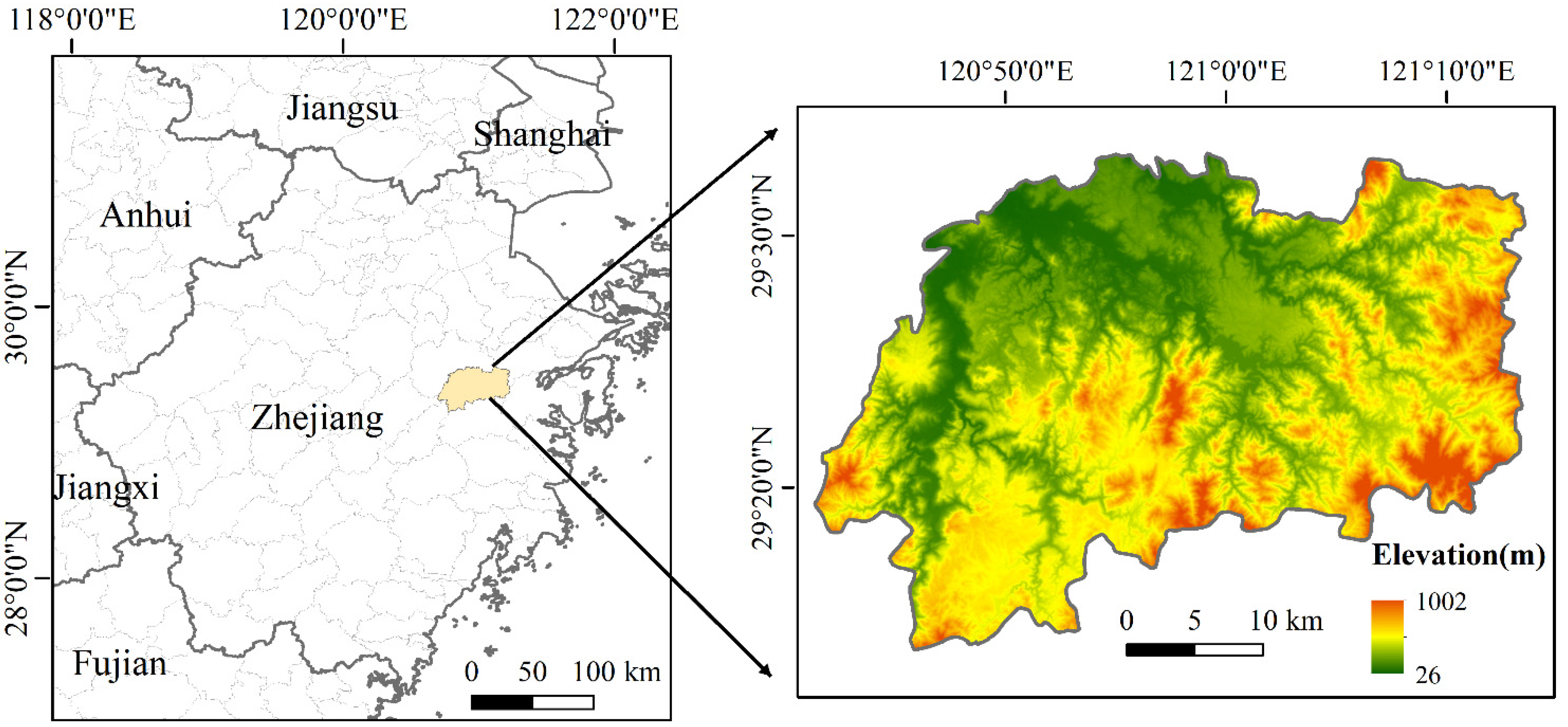
Figure 1. Overview of the study area in Xinchang, Zhejiang Province, China.
Agriculture 13 00010 g001
Figure 2. Structure of the R-CNN model. (a) CNN encoder, (b) CNN decoder, and (c) R-CNN.
Agriculture 13 00010 g002
Figure 3. Maps predicted from five distinct methods along with remote sensing images and the ground truth. (a) VHR images (acquired in December 2020), (b) ground truth maps, and the results from the (c) SVM, (d) RF, (e) CNN, (f) RNN, and (g) R-CNN methods. The green pixels represent the tea plantations, and the black pixels represent the non-tea plantations (other ground objects).
Agriculture 13 00010 g003
Figure 4. Confusion matrix for the spatial distribution of tea plantations in Xinchang County predicted by the (a) SVM, (b) RF, (c) CNN, (d) RNN, and (e) R-CNN methods.
Agriculture 13 00010 g004
Figure 5. Spatial distribution of tea plantations in Xinchang County predicted by the R-CNN method.
Agriculture 13 00010 g005
Figure 6. Distribution index of tea plantations in Xinchang County: (a) distribution index with elevation and (b) distribution index with slope.
Agriculture 13 00010 g006
Table 1. Spectral band specifications of Sentinel-2 remote sensing image.
Band NameCentral Wavelength (μm)Spatial Resolution (m)
B1—Coastal aerosol 0.443 60
B2—Blue0.49010
B3—Green0.56010
B4—Red0.66510
B5—Vegetation Red Edge 10.70520
B6—Vegetation Red Edge 20.74020
B7—Vegetation Red Edge 30.78320
B8—NIR0.84210
B8A—Narrow NIR0.86520
B9—Water vapor0.94560
B10—SWIR Cirrus1.37560
B11—SWIR 11.61020
B12—SWIR 12.19020
Table 2. Vegetation indices in input features.
NameCalculation Formulas
NDVI N D V I = B 8 B 4 B 8 + B 4
MNDVI M N D V I = B 4 B 3 B 4 + B 3
EVI E V I = 2.5 × B 8 B 4 B 8 + 6 × B 4 7.5 × B 2 + 1
NDVIre1 N D V I r e 1 = B 8 A B 5 B 8 A + B 5
NDVIre2 N D V I r e 2 = B 8 A B 6 B 8 A + B 6
NDVIre3 N D V I r e 3 = B 8 A B 7 B 8 A + B 7
Table 3. Hyperparameter settings of the experiment.
Initial Learning RateBatch SizeEpochLoss Function
0.0018200cross entropy loss
Table 4. F1 score and IoU achieved by different schemes of input features.
FeaturesF1IoU
Common bands0.7740.631
Common bands and red-edge vegetation bands0.8390.722
Common bands and SWIR bands 0.8210.697
All spectral bands0.8850.793
All spectral bands and vegetation indices0.8830.792
Table 5. F1 score and IoU achieved by various methods on the test dataset.
MethodF1IoU
SVM0.7740.632
RF0.8120.684
CNN0.8550.747
RNN0.8440.730
R-CNN0.8850.793
Table 6. Evaluation of the predicted spatial distribution of tea plantations in Xinchang County based on sample points.
MethodClassCE (%)OE (%)OA (%)Kappa
SVMTea 10.213.390.20.798
Others 9.67.3
RFTea 9.310.591.60.829
Others 7.76.7
CNNTea 7.57.493.70.871
Others 5.55.5
RNNTea 7.99.692.60.849
Others7.05.7
R-CNNTea 4.96.395.30.904
Others 4.63.5
Disclaimer/Publisher’s Note: The statements, opinions and data contained in all publications are solely those of the individual author(s) and contributor(s) and not of MDPI and/or the editor(s). MDPI and/or the editor(s) disclaim responsibility for any injury to people or property resulting from any ideas, methods, instructions or products referred to in the content.