Abstract
Achieving fast and accurate recognition of garlic clove bud orientation is necessary for high-speed garlic seed righting operation and precision sowing. However, disturbances from actual field sowing conditions, such as garlic skin, vibration, and rapid movement of garlic seeds, can affect the accuracy of recognition. Meanwhile, garlic precision planters need to realize a recognition algorithm with low-delay calculation under the condition of limited computing power, which is a challenge for embedded computing platforms. Existing solutions suffer from low recognition rate and high algorithm complexity. Therefore, a high-speed method for recognizing garlic clove bud direction based on deep learning is proposed, which uses an auxiliary device to obtain the garlic clove contours as the basis for bud orientation classification. First, hybrid garlic breeds with the largest variation in shape were selected randomly and used as research materials, and a binary image dataset of garlic seed contours was created through image sampling and various data enhancement methods to ensure the generalization of the model that had been trained on the data. Second, three lightweight deep-learning classifiers, transfer learning based on MobileNetV3, a naive convolutional neural network model, and a contour resampling-based fully connected network, were utilized to realize accurate and high-speed orientation recognition of garlic clove buds. Third, after the optimization of the model’s structure and hyper-parameters, recognition models suitable for different levels of embedded hardware performance were trained and tested on the low-cost embedded platform. The experimental results showed that the MobileNetV3 model based on transfer learning, the naive convolutional neural network model, and the fully connected model achieved accuracy of 98.71, 98.21, and 98.16%, respectively. The recognition speed of the three including auxiliary programs was 19.35, 97.39, and 151.40 FPS, respectively. Theoretically, the processing speed of 151 seeds per second achieves a 1.3 hm2/h planting speed with single-row operation, which outperforms state-of-the-art methods in garlic-clove-bud-orientation recognition and could meet the needs of high-speed precise seeding.
1. Introduction
Garlic is a globally cultivated crop due to its rich nutritional and medicinal value. According to 2022 statistical data from the FAO, the garlic planting area in China in 2020 was about 830,000 hectares, and garlic production reached 20 million tons, the largest in the world. However, the current mechanized planting of garlic is not efficient, and the sowing period of garlic is very short, so high-speed, high-efficiency, and accurate planters are urgently needed.
Many studies have shown that the orientation of garlic cloves buds during garlic sowing into the soil significantly affects the time and consistency of seedling emergence, garlic yield, and garlic bulb quality [1,2]. One study showed that when the garlic clove buds were facing upward and the inclination angle was within ±45°, all the indexes of garlic plants performed well. When the garlic clove buds were placed horizontally, the performance of each index was slightly inferior to that of the garlic clove buds facing upward. When the garlic clove buds were facing downward and the inclination angle was within ±45°, the performance of each index was the worst, making them prone to garlic seed necrosis, uneven seedling emergence time, disordered and weak growth, and other problems [3]. Therefore, the precise sowing of garlic first needs to meet the agronomic requirements of garlic planting with clove buds being placed upright.
Cangshan and Jinxiang garlic are the most widely cultivated garlic breeds in China. At present, existing garlic planters mostly adopt a righting mechanism to adjust the garlic clove bud direction. The garlic cloves of Cangshan are neat and uniform, and their weight, geometric shape, and the center of gravity are consistent, which could be utilized by a mechanical mechanism to achieve garlic bud upright sowing into soil [4,5]. Jinxiang garlic, the most commonly planted variety, is a hybrid breed with variable sizes of cloves, irregular geometric shape, and unstable center of gravity, and the mechanical righting method often has a poor effect [6]. The righting of hybrid garlic seeds remains an open problem, and beyond that, high-speed precision sowing requires shorter cycling time for righting seeds.
The correct recognition of garlic clove bud orientation is the foundation of garlic clove righting operation, and computer vision is the only feasible way to judge the clove bud orientation of hybrid breed garlic. In the early stage, some studies tried to use artificial feature engineering to solve the orientation recognition of garlic seeds, such as the density of edges [7], the position of centroid [8], the curvature of contour [9], etc. These methods are effective for garlic cloves with a standard shape, but poor for garlic cloves with residual garlic husks and abnormal spikes, while commercial garlic seeds often have residual husks and irregular geometric shapes, so the robustness of the artificial features engineering algorithm is not ideal, and the actual use is very poor.
At present, as automatic feature-learning methods, deep-learning methods perform well and have been widely used in the agricultural field [10], including in the orientation recognition of garlic clove buds [11]. However, some methods can only identify the position of qualified garlic clove buds, lack a description of unqualified positions, and cannot provide position information to support the righting operation of the garlic planter.
The above-mentioned studies are limited to the scope of algorithms and theory, while some other studies are focused on practical application, including the integration of algorithms in embedded hardware that can be equipped with garlic planters [12]. Li et al. designed an automatic righting device for garlic clove buds based on the Jetson Nano processor. The success rate of garlic clove bud righting of the device reached 96.25%, and when the number of parallel sowing rows was 12, its sowing efficiency was 0.099–0.132 hm2/h [13]. The righting method of Li et al. requires a Jetson Nano processor in each righting channel to achieve the planting efficiency of 0.099–0.132 hm2/h. However, the hardware cost of Jetson Nano is relatively high (US $99), so this design may not be conducive to commercial application.
So far, no research has tried to realize fast and accurate recognition of garlic seed orientation that can meet the needs of high-speed and accurate sowing of garlic with a low-cost embedded processor, and no research has attempted to solve the problem that the abnormal shape of garlic seeds, such as garlic skin residue, etc., affects orientation recognition. The above two research gaps hinder the practical application and large-scale promotion of machine-vision-based garlic seed orientation identification methods. Therefore, this paper proposes a robust, lightweight, and high-performance garlic bud orientation recognition method based on deep learning to achieve high-speed and accurate orientation recognition based on a single low-cost embedded processor.
Disturbances from actual field sowing conditions, such as garlic skin, vibration, and rapid movement of garlic seeds, can affect the accuracy of recognition. Meanwhile, garlic precision planters are in need of a recognition algorithm with a low delay calculation under the condition of limited computing power, which is a challenge for embedded computing platforms. In order to solve these problems, this study carried out the following work:
- Building of a special data set for model training, including shape anomalies such as garlic residue and motion blur, to ensure the generalization ability of the model to real scenes.
- Use of multiple deep-learning and feature-compression methods to realize garlic bud direction recognition and optimization of the model by tune operations.
- Performance tests of the models on low-cost embedded boards, selection of the optimal model, comparison with other methods to verify the superiority of this method.
The main contributions of this paper are as follows: an efficient method for obtaining a contour map is proposed, and a data enhancement method is proposed on this basis; quick-recognition models of lightweight CNN MobileNetV3 and naive CNN based on the contour map are proposed for high-speed recognition of garlic seed orientation; a high-speed contour orientation recognition method based on highly compressed contour features is proposed that realizes ultra-high-speed recognition on low-cost embedded platform.
Finally, a recognition speed of 151.40 FPS was achieved on the OrangePi 3 LTS, which can support sowing operations at a speed of 1.3 hm2/h, which is superior to the state-of-the-art method of garlic orientation recognition.
2. Materials and Methods
2.1. Garlic Clove Data Collection
In the field of deep learning, especially in image recognition, the collection of complete datasets that cover all application conditions is critical. The operator can judge the direction of a garlic clove bud mainly based on an outline of visual information. Based on this, the binary contour image of garlic seeds is used as the basis for judging the orientation of garlic cloves. Along with the support of a specific device, it is very easy to obtain an outline of garlic cloves. This paper used a strong light source as the background, obtained the shadow image and binary image of the garlic seed, and then applied the findcontours function of the graphics library OpenCV. This design has the following advantages: first, the binary contour image eliminates the imaging differences between different image sensors. Second, using a single-channel image as the input of the CNN model helps to reduce the amount of computation. Third, many traditional methods [7,9] also use contour images as input data, and using binary contours as model input is conducive to algorithm integration between different devices.
2.1.1. Garlic Clove Image Sample Collection
Deep learning requires that the training data and test data meet the conditions of being independent and identically distributed to ensure the generalization ability of the model. In the practical application stage of the model, the input data of the model must be independent and identically distributed with the training set in order to make the model work effectively. Therefore, considering the practical application of a deep learning model in a garlic planter, the training samples should cover wider morphological diversity distribution to enhance the robustness of model. When selecting training samples, one should not only ensure the garlic clove sizes, weights, and appearance, but also consider the influence of garlic seed production technology and other factors on garlic seed morphology, such as skin residue.
In this paper, the binary contour image was used as the model input, and the morphological features such as color and texture were discarded in the process of extracting the contours, while some edge features were preserved. Commercial garlic seeds are prone to having residual garlic skins and abnormal spikes. These garlic skin residues have a great impact on the extraction of contour images, and sometimes the extracted contour images may seriously deviate from the standard shape of garlic seeds. Therefore, the selection of training samples should also consider the situation of carried garlic skins while seeding. Because the individual shape of garlic cloves of hybrid garlic breed is the most diverse, we randomly selected Jinxiang garlic and divided it into cloves, retained all the garlic cloves without screening, and obtained a total of 735 garlic cloves for image samples. When dividing garlic cloves, about ½ of the skin residue of the garlic cloves was retained to ensure consistency with real sowing of garlic seeds, as shown in Figure 1a.
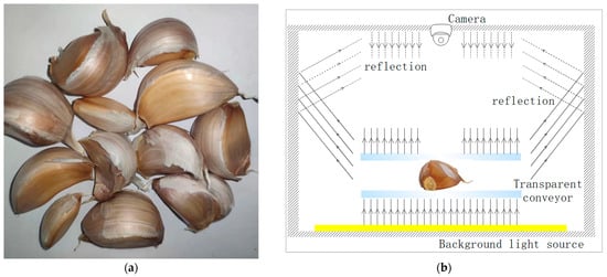
Figure 1.
(a) Garlic clove samples and (b) image acquisition device.
Sample Acquisition Device and Image Preprocessing
In order to directly obtain the contour images of the garlic cloves, a garlic seed shooting device was designed that uses a transparent clamping belt to clamp and transmit the garlic cloves and adopts the method of back illumination of area light source. The area light source is placed below the transparent clamping belt, and the image sensor is placed above the transparent clamping belt. The clamping transmission module is wrapped by an opaque shell to avoid the influence of external light on image acquisition. The light emitted by the area light source passes through a transparent clamping tape to form a clear garlic clove shadow image on the vision sensor, as shown in Figure 1b. The image collected under the ideal state is shown in Figure 2a. However, because the reflection in the shell cannot be completely eliminated, some reflected light will still be cast on the upper surface of the garlic clove, and the continuous transmission of the garlic clove will bring the dust that adhered to the garlic clove into the shell, reducing the contrast between the shadow area of the garlic clove and the background, as shown in Figure 2b.
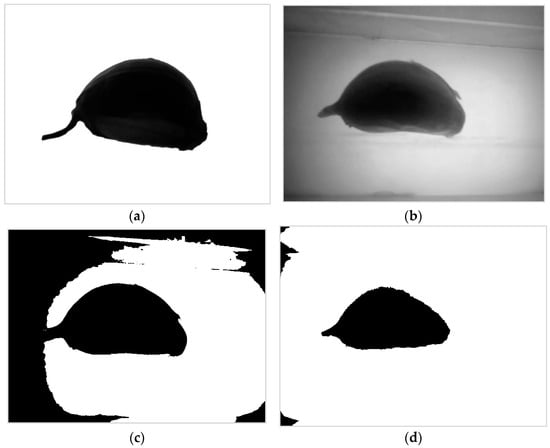
Figure 2.
The lighting environment in the device affects shadow imaging. (a) Idealized shadow image, (b) Actual shadow image, (c) Otsu-based binary image, (d) Fixed-threshold-based binary image.
The above situation increases the difficulty of binarization of shadow image. Because the shadow of the garlic seed image is too dark, the binarization performance to achieve contour is poor. Manually adjusting the binarization threshold can alleviate the problem of misclassifying the area around the shadow image, but the shadow of the garlic clove will be lost and cannot be applied automatically, as shown in Figure 2c,d. An extremely low-computation pixel compensation method is proposed to solve this problem. The control system records an image of the empty conveyor belt without cloves, and then calculates the pixel difference matrix between this image and a pure white image and saves it as a pixel compensation matrix. When intercepting the garlic clove shadow image frame, the intercepted image frame is added to the pixel difference matrix, and then the Otsu binarization method [14] is used to obtain a high-quality binarized image, as shown in Figure 3. The calculation rules are shown in Equations (1) and (2), where O represents the image with no load when the device is initialized; C stands for the pixel compensation matrix; X represents the image frame collected in real time; X’ represents the image frame after compensation; and m and n represent the number of rows and columns of the pixel matrix, respectively.
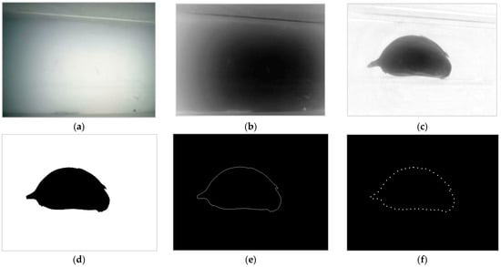
Figure 3.
Contour extraction after pixel compensation. (a) Background of conveyor, no clove, (b) Pixel compensation matrix, (c) Compensated garlic clove shadow, (d) Binary shadow image, (e) Outline of garlic seed, (f) Contour sampling points.
Dataset Acquisition Method
During the sample image acquisition, the mechanical device introduced in the previous section was used to transmit garlic seeds, the vision sensor on it was used to record a video, and then the image frames were extracted from the acquired video. A total of 1470 original image samples were obtained. Among them, 1172 images were randomly selected as the training set, and the remaining 298 images were used as the validation set. Since the length–width ratio of most image sensors is 4:3, when applied to the seeder, the long side of the picture was parallel to the travel direction of garlic seeds to obtain a larger observation field of garlic seeds. In order to meet this demand, the image samples used for model training were processed with the same length–width ratio and were finally saved with an image size of 640 × 480 by cutting or expanding the image boundary (Figure 4). Image rotation does not change the shape of garlic cloves. In this study, the original image samples were all adjusted to the upward state of garlic clove buds through image rotation operation. In the data enhancement stage, image samples with other orientations were generated through image rotation.
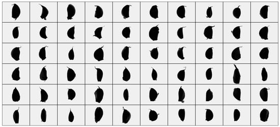
Figure 4.
Part of the original sample.
2.1.2. Data Enhancement for Datasets
Because the original images were adjusted to the garlic clove bud upward state, the key task in data enhancement was to generate image samples with left, bottom, and right orientation. In addition, some image transformations need to be performed on the image samples to make the images of the dataset more diverse to ensure the generalization ability of the model. In order to make the training data and the validation data conform to the conditions of independent and identical distribution, the same data augmentation operation was performed on the training samples and the validation samples, and the samples in the training set and validation set were always isolated during this process. The image enhancement methods include horizontal flipping, stretching, shearing, translation, rotation, and motion blur. All these methods except motion blur can be realized by two-dimensional geometric transformation, which can be completed by multiplying the pixel matrix of the image by a homogeneous transformation matrix. The mathematical expression of this process is shown in Equation (3). In order to enhance the generalization of the sample to the image acquisition environment in the garlic seeder, these methods need to follow a certain logical order.
where X represents the original image, and X’ represents the image after transformation; Mf, Ms, Md, Mt, and Mr represent the transformation matrix of horizontal inversion, stretching, shearing, translation, and rotation, respectively; w represents the width of the image; sx and sy represent the stretching ratio in two directions; dx and dy represent the shearing amplitude in two directions; tx and ty represent the translation distance in two directions; θ represents the rotation angle of the image.
Morphological Diversity
First, a flip operation on the image was performed. Due to the irregular shape of garlic cloves, they usually show different external contours when the two sides of their abdomen are facing vertically downward. Therefore, the diversity of the dataset can be increased through the horizontal flipping operation (Figure 5). After this operation, the sample size doubled to 2940.
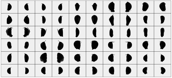
Figure 5.
Horizontal reversal amplification sample.
Then, stretch, shear, and translation were performed. These three operations can effectively increase the morphological diversity of the image and are still effective after image rotation. The stretching operation range was a random value in the range of 0–20%. The strength of the shear operation was a random value in the range of 0–10. The range of translation operation amplitude was a random value in the range of 0–10%. Through the overlapping operation of the above three transformations, the image samples were amplified to 29,400. The amplified samples are shown in Figure 6.
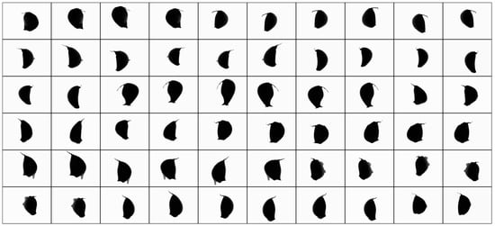
Figure 6.
Stretching, shearing, and translation.
Image Rotation and Class Generation
When the plane is divided into four equal regions, upper, left, lower and right, the range of each region is 90°. In order to ensure the generalization ability of the model for irregular orientation, before generating image categories, a random small-amplitude rotation operation was performed on the image samples. The rotation amplitude in the ideal state should be ± 45°, but the original image was manually rotated and righted, and there might be subtle deflection that is not easy to detect. Furthermore, because the data enhancement operation includes shear transformation of random amplitude, a rotation transformation in the range of ±30° was performed on each image, acting directly on the original image, without generating new image samples. The transformed samples are shown in Figure 7.
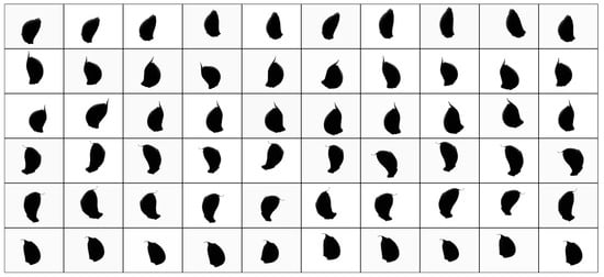
Figure 7.
Image samples after rotation in the range of ± 30°.
After completing the above operations, each original image was rotated by 90, 180, and 270° counterclockwise to obtain the standard left, lower, and right images. At this time, the sample size expanded to 117,600. The samples of each orientation class are shown in Figure 8.
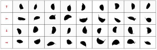
Figure 8.
Samples of each orientation class.
Motion Blur and Contour Extraction
Seeding speed is an important performance index of garlic seeders. In order to achieve high-speed seeding, garlic seed images should be collected in motion, which may lead to motion blur in the collected images. Because of the influence of uncertain motion blur on contour extraction, the data enhancement operation should also include motion blur with a certain probability and range. In this study, image samples were randomly selected with a probability of 50%, and motion blur with random amplitude was applied in the direction parallel to the long edge of the image (Figure 9).
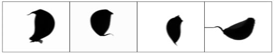
Figure 9.
Motion blur in different direction classes.
After all the data enhancement operations were completed, the contour of the image samples were extracted one by one, finally forming the garlic seed contour dataset for model training (Figure 10).
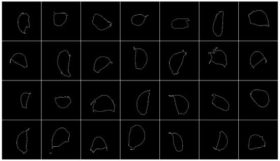
Figure 10.
Final generated outer contour image samples.
Logical Sequence of Data Enhancement Operations
If the rotation operation used to generate the orientation classification is performed before the zoom, stretch, shear, and translation operations, image samples with greater morphological differences can be generated, theoretically promote the generalization ability of the deep-learning model during training. However, it was found in experiments that datasets with the same orientation classification morphology have better performance. A possible reason is that when the four classifications contain samples with the same morphology, the deep learning model can suppress the influence of morphology on classification and pay more attention to the high-level semantic feature of “orientation”.
Because motion blur is directional, motion blur transformation should be carried out after rotation transformation, and motion blur may affect the edge contour, so contour extraction should be carried out after motion blur operation.
Storage of Dataset
The lightweight CNN model discussed has low computation complexity. A large batch size can be used in training on PC, and the training/inferring time of each batch is very short. In the initial practice, it was found that the transmission speed of training samples was often lower than the processing speed of the model; therefore, the way the dataset is stored has been improved. In the experimental environment of this paper, when using TFRecord format defined in TensorFlow [15] to store datasets, the input speed of samples could reach more than 10 times that of batch reading image files, which is faster than the inference speed of all deep learning models introduced in this paper. Therefore, this format is used as one of the storage schemes for datasets and testing of several CNN models.
The fully connected model proposed in Section 2.2.3 takes the pixel coordinates of garlic clove contours as the input. When the dataset composed of image samples is converted into the form of pixel coordinate array, the volume of the dataset is further reduced, and the whole dataset can be loaded into memory during training. The format DataFrame of Pandas [16] is used to store an array of contour point coordinates for all samples, which is changed to H5 format for loading on each training task. For the above two dataset formats, the shuffle operation was implemented for each training epoch to obtain better training results.
2.2. Lightweight Recognition Model of Garlic Clove Bud Orientation
For the garlic seed orientation recognition method studied in this paper, its accuracy is the first important criterion. Secondly, it is of practical significance to improve the running speed of the recognition model under the premise of ensuring accuracy. At the same time, the hardware cost of the algorithm application is also one of the factors considered in this paper, which is a necessary condition to ensure the generalizability of the application. Low hardware cost means low computing performance, so the complexity of the recognition model needs to be greatly reduced, which should be key for input features and lightweight models. Therefore, the main contribution of this paper is to propose a deep-learning model, that is, to improve the recognition rate and running speed of the model, give priority to ensuring the accuracy of the algorithm, and try to lighten the model on this basis to adapt to low-cost embedded platforms. The application of a convolutional network and a fully connected neural network in garlic-clove orientation recognition was attempted in this study. The convolutional network included MobileNetV3 [17] with relatively complex structure and the naive CNN model, composed of convolutional-pooling stacking only. These directly used garlic contour image samples as input, and automatically completed feature extraction through image convolutional operations. The fully connected model used the contour point coordinate set sampled from the image samples as the input, and the contour point sampling operation can be regarded as a feature extraction method.
2.2.1. Transfer Learning Based on MobileNetV3
MobileNetV3 is an excellent lightweight deep-learning model with two versions, large and small, which can be used as solutions for different levels of hardware performance. The TensorFlow framework comes with MobileNetV3 implementation code based on Keras API and provides six groups of pre-training parameters for training from an ImageNet dataset, which correspond to three forms of large and small models: standard width, 0.75 width, and standard width minimal mode. Based on this, transfer learning was tested.
The input size of the model is directly related to the amount of calculation required. In terms of ensuring the recognition performance of the model, the smaller the input size, the better. It was found in the experiment that when the image sample size was scaled to 120 × 160, the recognition performance of the model did not decrease significantly, so the input size of the MobileNetV3 model was modified to (120, 160, 1). The orientation of garlic clove buds was divided into four categories; the output size of the corresponding model is a 4-dimensional vector. Because the input and output of the model are redefined, only the weight values of the intermediate layers that are consistent with the original model parameter structure were loaded when loading the pre-training weights, and the intermediate layers with different structures were equivalent to training from zero.
Twelve model structures, including six with pre-training weights, were trained. The training results (Table 1) show that the transfer learning is effective. Using the pre-trained weights on the ImageNet dataset to perform transfer learning on the garlic seed outline, the image dataset could obtain a higher accuracy than starting training from zero. Overall, the large model performed better than the small model. The performance of the minimalistic mode was lower than that of the non-minimalistic mode, but this gap was not noticeable when pre-trained weights were not used. By comparing the number of parameters and calculation of different models, it can be seen that reducing the width factor mainly reduces the amount of calculation required for the model, which can improve the running speed of the model, while the minimalistic mode mainly reduces the number of parameters of the model, which can reduce the memory consumption of the model. The accuracy rate of all the model forms can reach above 0.96, and they all have certain application value. The structure of MobileNetV3-Large is shown in Figure 11.

Table 1.
Overview of the performance of the transfer learning model.
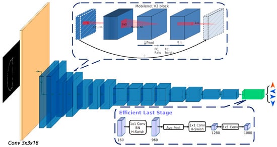
Figure 11.
Structure of MobileNetV3.
2.2.2. Naive CNN Model
Compared with classic CNN models such as AlexNet [18] and VGG NETS [19], MobileNetV3 has a relatively complex model structure, and includes some advanced designs, such as depthwise separable convolution [20], inverse residual block structure [21], squeeze-and-excitation block [22] and h-swish [17] activation function. Along with their support, MobileNetV3 shows excellent classification performance for some large-scale natural image datasets. The garlic contour image is very different from natural images. As a binary image, its content density and information density are very low. In order to explore which designs of MobileNetV3 are most helpful to the classification task of garlic contour images, some experiments were done. By training a modified model that separately applies the squeeze-and-excitation module, h-swish activation function, and 5 × 5 convolution kernel, this study found that the 5 × 5 convolution kernel had the greatest impact on model performance among the three, while the squeeze-and-excitation and the h-swish activation function had little effect on model performance. After determining the importance of convolutional kernel size, a series of naive CNN models with a structure similar to VGG NETS were constructed, which were compared with MobileNetV3 to analyze the impact of inverse residual block structure on the performance of the model and further verify the importance of convolutional kernel size.
In order to make the training results of the models more comparable, the same training conditions as MobileNetV3 transfer learning were used to train these models. The performance achieved after full convergence is shown in Table 2. Because these models have a simple structure, compared with the MobileNetV3 model, the parameters and calculation of the naive CNN model with similar performance are greatly reduced. This seems to indicate that the model with a simple structure is more suitable for solving the direction judgment problem of garlic clove contour images, but the naive CNN model does not match the performance achieved by MobileNetV3-Large transfer learning using the same training strategy.
Table 2.
List of Naive CNN models.
The performance of the naive CNN model provides some guidance for the optimization of the model. Comparing model 1 and model 2 in Table 2, there is a large gap in the performance of the model when the number of channels of each convolutional layer is doubled. It can be seen that ensuring the width of the model is one of the key factors to improve the performance of the model, but the cost of doubling the width is high, and the number of parameters and calculations is doubled. Comparing model 2 and model 3, it is further verified that the convolutional kernel of 5 × 5 is more efficient than the convolutional kernel of 3 × 3, and because of the depthwise separable convolution, the increase in the number of parameters and calculation is not large. Comparing model 4 and model 5, the max-pooling operation is more reliable than the down-sampling method using a convolutional layer with a step size of two as a characteristic graph. Comparing model 3 and model 6, the position of the lower sampling layer in the model will also affect the performance of the model. In general, the low layer of the model (close to the input layer) does not need to stack too many convolutional layers, while the high layer of the model (close to the output layer) needs to stack more convolutional layers.
2.2.3. Contour-Resampling-Based Fully Connected Network
Because the information density of the binarized contour image samples is extremely low, using CNN to solve the classification problem of such images seems to be a waste of performance, so another solution was tried.
The contour image samples in the dataset can be represented as a coordinate set of contour pixel points that only contains elements twice the number of contour pixel points (horizontal and vertical coordinate values). The number of contour pixels in some 480 × 640 size contour maps is counted, and the number of contour pixels is within 800, while the total number of pixels in the overall contour map is up to 307,200. Therefore, the set of contour point coordinates of each image sample is used as the model input, and building a fully connected neural network can also solve the orientation recognition problem of garlic clove contour images. Although this method needs to increase the steps of extracting contour points from the collected image, the increased amount of calculation is very small. Along with the help of OpenCV, the extraction process of contour points is also very easy to implement.
Uniform Input Size
It is very difficult to realize the variable length input of a neural network. Because the number of contour pixels contained in each contour image sample is different, it is necessary to unify the number of contour pixels of the sample first. Hence, the equidistant sampling method is used to sample a fixed number of point coordinates from the contour of each image, and then draw a polygon with these sampled points and observe its ability to reconstruct the original sample through artificial vision (Figure 12). It was found that when 50 contour points were sampled, the polygon formed was very close to the shape of the original sample. Through the above sampling method, 50, 100, and 200 contour point sets of all contour image samples were collected and combined with the orientation classification of the samples as the training dataset of the fully connected model. A fully connected model with three Hidden layers and 512, 256, and 128 neurons was used for testing. It was found that there was no significant difference in the recognition rate of the model when 200, 100, or 50 sampling points were used, but using fewer sampling points could effectively reduce the number of parameters and calculations of the model, so 50 points is preferable.
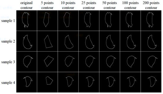
Figure 12.
The ability of contour points with different sampling rates to restore the original contour.
The matrix shape of the contour point set obtained by the findcontours function of OpenCV is [n, 2], where n is the number of contour points, and the matrix shape of the contour point set after sampling is [m, 2], where m is the number of sampling points, and the dimension with length of 2 contains the horizontal and vertical coordinates of each contour point. For the fully connected model discussed in this section, the input of each layer of the model should be a one-dimensional vector, so it is necessary to flatten the contour point set. There are two ways to flatten: the first from the point dimension, the other from the coordinate dimension. The first flattening method was chosen (the value of the data_format parameter corresponding to the Keras Flatten layer is “channels_last”).
Structure of Fully Connected Model
Through the testing of several fully connected models defined by Keras API, it was found that when the number of Hidden layers of the model was less than three, increasing the number of fully connected layers was effective. When the number of layers exceeded three, increasing the number of fully connected layers could not significantly improve the recognition rate of the model. Using more neurons can improve the performance of the model, but increasing the number of neurons will greatly increase the number parameters of the model, resulting in the model becoming bloated. The preliminary test results of typical models are shown in Table 3. The accuracy of the model with 4096, 2048, and 1024 neurons in the Hidden layer reached 0.97893. The accuracy of the model with 1024, 512, and 256 neurons in the Hidden layer was 0.97465. The accuracy of the model with 512, 256, and 128 neurons in the Hidden layer was 0.97241.
Table 3.
Overview of fully connected models.
The structure of the fully connected model is shown in Figure 13. Each fully connected layer includes a batch normalization [23] layer. It is particularly noteworthy that adding batch normalization layers after the flat layer can greatly improve the convergence speed of the model.
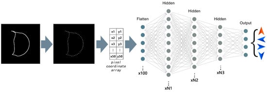
Figure 13.
Fully connected model. Note: both the Flatten and Hidden layers are connected to the Batch Normalization layer, but only the Batch Normalization layer of the Hidden layer applies the activation function. N1, N2 and N3 are the number of undetermined Hidden layer neurons.
2.2.4. Model Optimization
In order to obtain faster computing speed and higher accuracy, the three deep learning models have been greatly optimized, and the optimization directions include model lightweighting and model training tuning.
Implementation of Lightweight Convolutional Model
It was found that when the size of the input image of MobileNetV3 was reduced to 60 × 80, the recognition rate of the model decreased significantly, while in the relevant test of the naive CNN model, the input of 60 × 80 did not greatly reduce performance of the model.
The stride of the first standard convolution layer of the MobileNetV3 model is 2. When it was modified to 1, the performance of small-sized input of 60 × 80 was improved. Removing the 1 × 1 standard convolutional layer before the Global Average Pooling [24] layer did not reduce the recognition rate of the model, but it could reduce the number of parameters and computation of the model and improve the convergence speed of the model.
For the naive CNN model, the actual receptive field of the 3 × 3 convolutional kernel when using the input size of 60 × 80 was larger than the actual receptive field of the 5 × 5 convolution kernel when using the input size of 120 × 160. Since the edge of the garlic contour image is a background does not contain anything, the convolutional layers in the first two groups of the convolutional-pooling modules could be modified to valid padding. Due to the above adjustments and halved input size, two convolutional-pooling modules can be removed to achieve the same feature map size, which can greatly reduce the number of parameters and computations in the model. Since the input of the model is only a single-channel image, the use of standard convolution at the input of the model only increases the number of calculations and parameters by very little compared with the depthwise separable convolution. This change has been tested to slightly improve the performance of the model. The naive CNN model structure obtained after the abovementioned optimization procedure is shown in Figure 14.
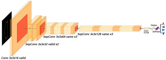
Figure 14.
Naive CNN model after lightweighting.
Model Training and Tuning
Three optimizers: Adam [25], Nadam [26], and SGD were tested in model training. The final convergence results of Adam’s optimizer in multiple training tests of the same model were unstable. Nadam and SGD were more stable than Adam, but Nadam had the greatest computational complexity of the three and the slowest performance. SGD is theoretically less efficient than Adam and Nadam, but the fully connected model proposed in Section 2.2.3 could converge stably when the learning rate of SGD was set to 1.0 or even higher. In this way, both the convergence speed of the model and convergence stability could be guaranteed. In addition, the computational complexity of SGD was the lowest of the three, and the computational speed was the fastest.
Five activation functions comprising Tanh, Relu6 [27], Gelu [28], Swish [29], and h-swish [17] were tested, and the convergence curve for the fully connected model is shown in Figure 15. When using the SGD optimizer, the effect of swish and h-swish was better (1000-epochs validation set accuracy is 0.97611 and 0.97586, respectively), and because the computational complexity of Hard-Swish was lower than that of Swish, and the model using h-swish was more reliable in weight value quantization, the fully connected model uses the h-swish activation function.
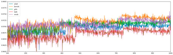
Figure 15.
Convergence curves of different activation functions. Note: the above convergence curves were all measured on the fully connected model proposed in Section 2.2.3, and the range shown in the figure is 100 to 1000 epochs.
For the garlic seed contour dataset, the training loss values of the three types of models tested are close to 0 in the later stage of the training process, the training set accuracy can be close to 100%, and the validation set accuracy is different. This is an overfitting phenomenon, and the loss flooding method [30] has a significant effect on it. The idea of this method is to keep the training loss value always above a certain threshold delta, so that the model can continue to learn and possibly converge to a better performing state. In the optimization process of the model, there may be a large number of local optimum points. The random walk strategy of the loss flooding method requires the optimizer to have a large enough optimization stride to ensure that the model escapes the local optimum point. When the model is optimized to a good state range, the weight value needs to be saved in time to prevent missing the state. In the later stages of the finite number of training iterations, the probability of the random walk method obtaining a better state becomes very low, but continuing to train the model with a smaller learning rate can often make the model’s performance improve again in the short term, so the learning rate decay method combined with the loss flooding method is very effective. In order to ensure that the model is in an ideal state when the learning rate decay is triggered, a program is written to dynamically load the weights saved during the last state boost each time the learning rate decays.
The LSR [31] method was also used. When the LSR method was applied alone, the model was trained with a label_smoothing parameter of 0.2, and the obtained validation set accuracy was comparable to the loss flooding method with a delta of 0.1. When the loss flooding method was combined with the LSR method, the delta and label_smoothing parameters were set to 0.7 and 0.2, and the accuracy of the validation set obtained was slightly improved, but the accidental components were not excluded.
Based on the above methods, L1/L2 regularization and Dropout [32] regularization were further tried. L1/L2 regularization is effective for convolutional models, but not for fully connected models. Dropout regularization looks simple and crude, but it significantly improves the performance of the fully connected model.
2.3. Application Method in Embedded System
The application of deep learning models in seeders requires some additional support programs and control programs. First, the deep-learning model will give a direction judgment for any input image, including the image when no garlic seeds pass by. Therefore, in order to avoid meaningless direction judgment and device linkage, for each frame of a collected image, a judgment should be made on whether it contains garlic seeds. Secondly, since the deep learning models constructed in this paper are all based on the contour image of garlic seeds or their sampling point sets as the basis for classification, an additional program is required to extract binarized contour image or resampling the contour points. A flow chart of the complete orientation judgment process is shown in Figure 16.
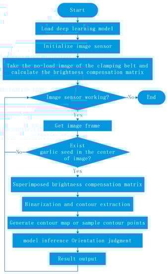
Figure 16.
Flow chart of orientation judgment procedure.
Under backlight illumination, it can be judged whether a garlic seed is passing by monitoring the change of the average pixel value of the central area of the camera’s field of view. Figure 17 shows the relationship between the average pixel value and the movement of a garlic seed in the camera’s field of view. When a garlic seed passes through the camera’s field of view, it is captured with multiple frames of images, then compared to the image frames of single garlic seed, and an image with the lowest average pixel value in the central area is obtained, which is the optimal image frame. This process is shown in Figure 18.
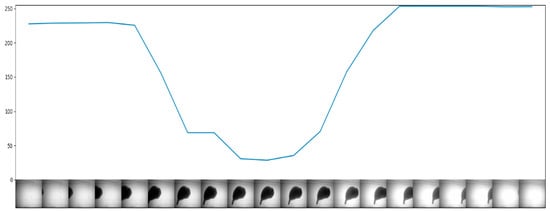
Figure 17.
Relationship between the pixel mean value of the central area of the field of view and the position of garlic seeds.
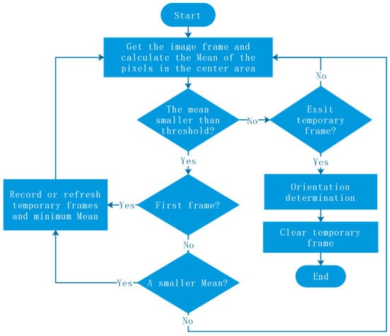
Figure 18.
Frame retrieval flow chart.
After obtaining the optimal image frame, brightness compensation is performed, binarization of the image is completed, and the contours from the binarized image are extracted. The output of the contour extraction algorithm is a set of contour points. For the CNN model that takes the contour image as input, the set of contour points needs to be drawn as a contour image. For the fully connected model that takes the set of contour points as input, it is necessary to reduce the number of contour point coordinates to a number suitable for the input of the model through sampling.
3. Results and Discussion
3.1. Model Test and Result
After a series of optimization operations, some typical models were retrained, and their performances are shown in Table 4. Of these models, the transfer learning model based on MobileNetV3-Large has the highest recognition rate of 98.71% on the validation set. However, compared to other models in Table 4, MobileNetV3-Large is too bloated. The recognition rate of the standard-width MobileNetV3-Small model is second only to the MobileNetV3-Large model, but its parameters and computation are still too large. The naive CNN model in Figure 14 performs better than the MobileNetV3-Small with reduced width factor, and its performance is close to that of the standard-width MobileNetV3-Small, but it has the lowest number of parameters among all the models in the table. The fully connected model with 512, 256, and 128 neurons in the Hidden layer achieves almost the same accuracy as the naive CNN model with extremely low computational cost and parameter cost. It has the fastest speed and the most cost-effective application.
Table 4.
Performance of the optimized model.
The last column of Table 4 shows the macro F1 score of the models. The F1 score of the four models are almost equal to the accuracy rate, which indicates that the recognition rate of the models for the four orientation categories are very balanced. The ROC curve and AUC value of the models also support this point. The ROC curves of the four orientations are almost identical with only a small gap, and they cover each other in the graph and are difficult to distinguish, as shown in Figure 19. Meanwhile, the macro average AUC and the AUC of each classification are close to 1, which indicates that the recognition effect of the models for each orientation classification are very good.
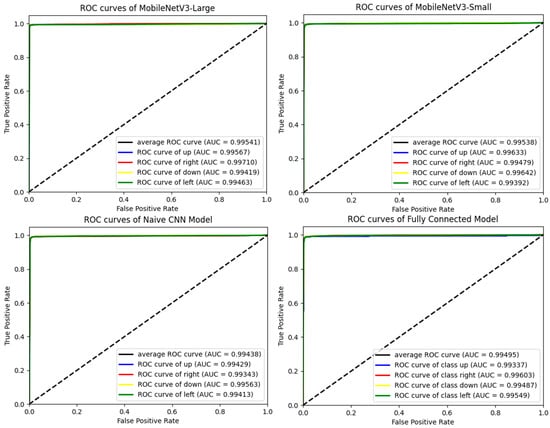
Figure 19.
ROC and AUC for models with recognition rates over 98%.
Based on the program flow introduced in Section 2.3, representative experimental models were selected and converted to TFlite format for speed testing on OrangePi 3 LTS. The test results are shown in Table 5. For the three CNN models in the table, due to their own calculation being more complicated, adding the complete process has little impact on its speed. The fully connected model itself has simple calculation and fast inference speed, but the ability of the support program to provide input data for the model is limited, and it finally reached a speed of about 151.40, which is still more than 50% faster than the fastest CNN model.
Table 5.
Inference speed of the model on OrangePi 3 LTS.
3.2. Discussion
3.2.1. Reliability Verification Experiment
In order to verify the validity of the data and model, a program was written to rotate the image samples 90° counterclockwise before extracting the contours and then extract the contour to identify its orientation, as shown in Figure 20. Since the original orientation categories up, left, bottom, and right correspond to labels 0, 1, 2, and 3 respectively, the category labels output by the model after the rotation should be 1, 2, 3, and 0. In the test, all the tested models can achieve almost the same recognition rate as before the sample rotation, as shown in Table 6.
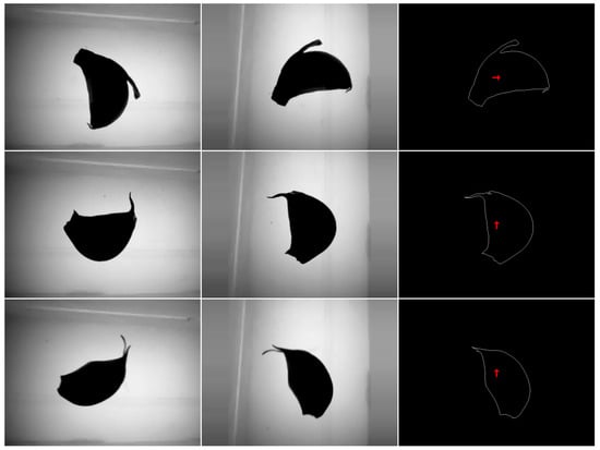
Figure 20.
Sample rotation test of the model.
Table 6.
Orientation recognition rate of the model to the rotated sample.
3.2.2. Comparison with Statistical Learning
The difficulty in applying statistical learning methods to image recognition is how to extract image features. The method of sampling fixed coordinate points at equal intervals of contour lines introduced in Section Uniform Input Size greatly reduces the feature dimension of the image, which can be regarded as a kind of feature extraction method. Based on this, several statistical learning algorithms such as KNN, SVM, and lightGBM [33] were fitted and tested using a dataset of 50 contour sampling points, but none of them matched the classification performance of the neural network algorithm.
In the test of the KNN algorithm, the NCA [34] algorithm is used to reduce the dimension of the data samples of 50 sampling points to generate a vector of a specific dimension and use it as the input of the KNN algorithm. In the parameter adjustment test, when the dimension of the model input vector, that is, the NCA output vector, was reduced to 25, and the number of adjacent elements of the KNN model is 16, the recognition rate of the validation set of the KNN model reaches a peak at 93.70%.
In the test of the SVM algorithm, the performance of the RBF kernel function was significantly higher than that of linear and poly kernel functions. The randomized search CV method was used to select C and gamma parameters. When C is 98.21 and gamma is 0.0044, the accuracy of the validation set of the SVM model reaches 94.06% of the optimal figure in the experiment.
In the test of the lightGBM algorithm, PCA algorithm was used to reduce the dimension of data samples at 50 sampling points. When the dimension of data samples was reduced to 25, num_leaves and max_depth parameter of the lightGBM algorithm were 127 and 8, respectively, and the recognition rate of the validation set of the lightGBM model could reach an optimal 96.56% in the experiment.
If PCA is not used, the lightGBM model can only achieve a recognition rate of less than 92% of the validation set, which indicates that the processing of the PCA algorithm not only reduces the dimension of the sample vector but also improves the ability of the data to represent the original sample. After follow-up tests, the improvement of model accuracy by PCA preprocessing is limited to gbdt-based algorithms such as XGBoost [35] and lightGBM and cannot greatly improve the recognition rate of validation sets of KNN, SVM, and fully connected neural networks. Using PCA to convert the coordinate data of 50 sampling points into a 25-dimensional vector can reduce the complexity of the model. For the fully connected model in Table 4, after modifying the model input to a 25-dimensional vector, the number of parameters was reduced to 183.6 K. The amount of computation was reduced to 0.36 M, but the recognition rate on the validation set dropped to 97.97%.
As a comparison, the accuracy and running speeds of KNN, SVM, lightGBM, and the fully connected model on the embedded platform are shown in Table 7. Obviously, the speed of the fully connected model is better than that of the statistical learning model.
Table 7.
Performance comparison of statistical learning models and fully connected model.
3.2.3. Comparison with Methods in Other Literature
Table 8 lists the garlic orientation recognition methods and their recognition rates described in the literature in recent years. It can be seen that the recognition rate of the method proposed in this paper is higher than other methods. Since all these studies use private datasets, this horizontal comparison is only for reference. However, because the samples contained in the dataset constructed in this paper uniquely retain the common morphological abnormalities and motion blur phenomena in the real scene, the reliability of the recognition rate achieved by the model in this study is at least not lower than that of other studies.
Table 8.
Comparison of recognition rate of methods in related literatures.
The generally high recognition rates of the models proposed in this paper indicate that the dataset enhancement method and the contour-image-based garlic-clove-bud orientation recognition models adopted in this paper are effective. The form of binarized contour image unifies the pixel value distribution of contour points, so that the information of image samples can be completely expressed by the coordinate set of contour points. The feature extraction method of contour point equidistant sampling further reduces the dimension of the input data, so that the extremely lightweight fully connected neural network can also complete the orientation classification task of garlic seeds with high accuracy and speed.
3.2.4. Application Prospect
The operating speed of the garlic planter can be calculated by Equation (4), where η represents the sowing efficiency (hm2/h), w represents the plant spacing (m), h represents the row spacing (m) and v represents the sowing speed (pieces/second).
The garlic sowing efficiency of the existing garlic seed adjustment method is in the range of 0.05–0.2 hm2/h [36,37]. According to the planting standards of 0.2 m row spacing and 0.12 m plant spacing, the four orientation recognition models in Table 5 can reach sowing speeds of 0.16, 0.51, 0.84, and 1.30 hm2/h, respectively. The above speed is the ideal single-row seeding speed. It can also be used in multi-row seeders in the form of controlling multiple rows through a single board. It only needs a single embedded board with the same performance as the OrangePi 3 LTS. If there are performance bottlenecks in the other devices that make up the garlic planter, the hardware configuration can be further reduced, thereby reducing the manufacturing cost of the planter.
4. Conclusions
To meet the need of high-speed garlic seed righting operations and low-cost onboard embedded computing platforms, the contour-based multiple lightweight deep-learning models including transfer learning based on MobileNetV3, naive CNN model, and a contour resampling-based fully connected neural network are proposed for garlic-clove-bud orientation recognition and tested by the image garlic seed samples with the same conditions as a field planter, and the best model was selected for parameter optimization. All of the models’ recognition rate of garlic clove bud orientation exceeded 98%. The MobileNetV3 model based on transfer learning, the naive CNN model, and the fully connected model achieved accuracy of 98.71, 98.21, and 98.16%, respectively, all far exceeding statistical learning methods. The parameters of the three are 4.04 M, 61.9 K, and 220.4 K, respectively. The calculation amount of the three is 0.178 G, 17.9 M, and 0.44 M FLOPs, respectively. The recognition speed of the three including auxiliary programs is 19.35, 97.39, and 151.40 FPS, respectively.
Experimental results showed that the contour-image-based garlic-clove-bud orientation recognition method is effective. The form of binarized contour image unifies the pixel value distribution of contour points, so that the information of garlic clove samples can be completely expressed by the coordinate set of contour points. Resampling of contour points further compresses sample features and simplifies the structure of deep-learning models. Ideally, a fully connected neural network based on contour resampling could support a seeding rate of 1.3 hm2/h. Therefore, the garlic-clove-bud orientation recognition based on deep learning proposed by this paper can meet the needs of high-speed and accurate sowing of garlic.
The main goals of this research for the future are to complete the integration of garlic species orientation recognition algorithm and orientation device, verify the effect of system integration, and continuously improve the device; collect more garlic seed contour image samples to join the dataset and train the model to continuously enhance its generalization ability; and try to generalize the orientation recognition algorithm proposed in this paper to other problems in the agricultural field.
Author Contributions
J.L.: writing—original draft, writing—review and editing, conceptualization, methodology, investigation, data curation, formal analysis, software, and validation. J.Y.: writing—original draft, writing—review and editing, funding acquisition, software and production of related equipment. J.C.: investigation, device design, and production of related equipment. Y.L.: investigation, data curation, validation, and production of related equipment. X.L.: writing—review and editing, funding acquisition, project administration. All authors have read and agreed to the published version of the manuscript.
Funding
This research was funded by cotton industry technology system and industrial innovation team projects in Shandong Province (SDAIT-03-09) and supported by the National Natural Science Foundation of China (51675317).
Institutional Review Board Statement
Not applicable.
Informed Consent Statement
Not applicable.
Data Availability Statement
Anyone can access the data by sending an email to jyuan@sdau.edu.cn.
Conflicts of Interest
The authors declare no conflict of interest.
References
- Ahn, Y.; Choi, G.; Choi, H.; Yoon, M.; Suh, H. Effect of planting depth and angle of non-cloved bulb garlics on the garlic growth and yield. Korean J. Hortic. Sci. Technol. 2007, 25, 82–88. [Google Scholar]
- Jin, C.; Yuan, W.; Wu, C.; Zhang, M. Experimental study on effects of the bulbil direction on garlic growth. Trans. CSAE 2008, 24, 155–158. [Google Scholar]
- Liu, J. Effects of Different Garlic Varieties and Bulbil Seeding Directions on Growth Characteristic and Quality. Master’s Thesis, Shandong Agricultural University, Tai’an, China, 2018. [Google Scholar]
- Huang, H.S. Numerical Simulation and Experimental Study on the Adjusting Device and Inserting Device of Double Duckbill Garlic Planter. Master’s Thesis, Shandong Agricultural University, Tai’an, China, 2019. [Google Scholar]
- Zhang, X.; Yi, S.; Tao, G.; Zhang, D.; Chong, J. Design and Experimental Study of Spoon-Clamping Type Garlic Precision Seeding Device. Wirel. Commun. Mob. Comput. 2022, 2022, 5222651. [Google Scholar] [CrossRef]
- Tian, L. Design and Experiment of Garlic Seed Orientation Device Based on Image Recognition Technology. Master’s Thesis, Shandong Agricultural University, Tai’an, China, 2020. [Google Scholar]
- Wu, X.; Hu, W. Research on Garlic Clove Orientation Recognition Based on Observation Window. Meas. Control. Technol. 2016, 35, 35–39. [Google Scholar]
- Zhao, L.Q.; Song, W.; Yin, Y.Y.; Zhou, C. System of Garlic Shape Recognition Based on Vision Technology. J. Agric. Mech. Res. 2014, 36, 206–208, 212. [Google Scholar]
- Guo, Y.F.; Lu, B.Y. Research on the Identification of the Roots of Garlic Based on SUSAN Algorithm. J. Yangling Vocat. Tech. Coll. 2011, 10, 1–4. [Google Scholar]
- Kamilaris, A.; Prenafeta-Boldú, F.X. Deep learning in agriculture: A survey. Comput. Electron. Agric. 2018, 147, 70–90. [Google Scholar]
- Fang, C.; Sun, F.Z.; Ren, C.G. Identifying bulbil direction of garlic based on deep learning. Appl. Res. Comput. 2019, 36, 598–600. [Google Scholar]
- Hou, J.L.; Tian, L.; Li, T.H.; Niu, Z.R.; Li, Y.H. Design and experiment of test bench for garlic bulbil adjustment and seeding based on bilateral image identification. Trans. CSAE 2020, 36, 50–58. [Google Scholar]
- Li, Y.H.; Liu, Q.C.; Li, T.H.; Wu, Y.Q.; Niu, Z.R.; Hou, J.L. Design and experiments of garlic bulbil orientation adjustment device using Jetson Nano processor. Trans. CSAE 2021, 37, 35–42. [Google Scholar]
- Otsu, N. A threshold selection method from gray-level histograms. IEEE Trans. Syst. Man Cybern. 1979, 9, 62–66. [Google Scholar]
- Abadi, M.; Agarwal, A.; Barham, P.; Brevdo, E.; Chen, Z.; Citro, C.; Corrado, G.S.; Davis, A.; Dean, J.; Devin, M. Tensorflow: Large-scale machine learning on heterogeneous distributed systems. arXiv 2016, arXiv:1603.04467. [Google Scholar]
- McKinney, W. Data structures for statistical computing in python. In Proceedings of the 9th Python in Science Conference, Austin, TX, USA, 28 June–3 July 2010; pp. 51–56. [Google Scholar]
- Howard, A.; Sandler, M.; Chen, B.; Wang, W.; Chen, L.-C.; Tan, M.; Chu, G.; Vasudevan, V.; Zhu, Y.; Pang, R. Searching for MobileNetV3. In Proceedings of the 2019 IEEE/CVF International Conference on Computer Vision (ICCV), Seoul, Korea, 27 October–2 November 2019; pp. 1314–1324. [Google Scholar]
- Krizhevsky, A.; Sutskever, I.; Hinton, G.E. Imagenet classification with deep convolutional neural networks. Adv. Neural Inf. Processing Syst. 2012, 25, 1097–1105. [Google Scholar] [CrossRef]
- Simonyan, K.; Zisserman, A. Very deep convolutional networks for large-scale image recognition. arXiv 2014, arXiv:1409.1556. [Google Scholar]
- Sifre, L.; Mallat, S. Rigid-motion scattering for texture classification. Comput. Sci. 2014, 3559, 501–515. [Google Scholar]
- Sandler, M.; Howard, A.; Zhu, M.; Zhmoginov, A.; Chen, L.-C. Mobilenetv2: Inverted residuals and linear bottlenecks. In Proceedings of the IEEE Conference on Computer Vision and Pattern Recognition, Salt Lake City, UT, USA, 18–23 June 2018; pp. 4510–4520. [Google Scholar]
- Hu, J.; Shen, L.; Sun, G. Squeeze-and-excitation networks. In Proceedings of the IEEE Conference on Computer Vision and Pattern Recognition, Salt Lake City, UT, USA, 18–23 June 2018; pp. 7132–7141. [Google Scholar]
- Ioffe, S.; Szegedy, C. Batch normalization: Accelerating deep network training by reducing internal covariate shift. In Proceedings of the International Conference on Machine Learning, Lille, France, 7–9 July 2015; pp. 448–456. [Google Scholar]
- Lin, M.; Chen, Q.; Yan, S. Network in network. arXiv 2013, arXiv:1312.4400. [Google Scholar]
- Kingma, D.P.; Ba, J. Adam: A method for stochastic optimization. arXiv 2014, arXiv:1412.6980. [Google Scholar]
- Timothy, D. Incorporating nesterov momentum into adam. Nat. Hazards 2016, 3, 437–453. [Google Scholar]
- Howard, A.G.; Zhu, M.; Chen, B.; Kalenichenko, D.; Wang, W.; Weyand, T.; Andreetto, M.; Adam, H. MobileNets: Efficient convolutional neural networks for mobile vision applications. arXiv 2017, arXiv:1704.04861. [Google Scholar]
- Hendrycks, D.; Gimpel, K. Gaussian error linear units (gelus). arXiv 2016, arXiv:1606.08415. [Google Scholar]
- Ramachandran, P.; Zoph, B.; Le, Q.V. Searching for activation functions. arXiv 2017, arXiv:1710.05941. [Google Scholar]
- Ishida, T.; Yamane, I.; Sakai, T.; Niu, G.; Sugiyama, M. Do we need zero training loss after achieving zero training error? arXiv 2020, arXiv:2002.08709. [Google Scholar]
- Szegedy, C.; Vanhoucke, V.; Ioffe, S.; Shlens, J.; Wojna, Z. Rethinking the inception architecture for computer vision. In Proceedings of the IEEE Conference on Computer Vision and Pattern Recognition, Las Vegas, NV, USA, 27–30 July 2016; pp. 2818–2826. [Google Scholar]
- Srivastava, N.; Hinton, G.; Krizhevsky, A.; Sutskever, I.; Salakhutdinov, R. Dropout: A simple way to prevent neural networks from overfitting. J. Mach. Learn. Res. 2014, 15, 1929–1958. [Google Scholar]
- Ke, G.; Meng, Q.; Finley, T.; Wang, T.; Chen, W.; Ma, W.; Ye, Q.; Liu, T.-Y. Lightgbm: A highly efficient gradient boosting decision tree. In Proceedings of the Advances in Neural Information Processing Systems 30 (NIPS 2017), NeurIPS, Long Beach, CA, USA, 4–9 December 2017; Volume 30. [Google Scholar]
- Goldberger, J.; Roweis, S.; Hinton, G.; Salakhutdinov, R. Neighbourhood components analysis. In Proceedings of the 17th International Conference on Neural Information Processing Systems; 2004; pp. 513–520. Available online: https://dl.acm.org/doi/10.5555/2976040.2976105 (accessed on 4 August 2022).
- Chen, T.; Guestrin, C. Xgboost: A scalable tree boosting system. In Proceedings of the 22nd Acm Sigkdd International Conference on Knowledge Discovery and Data Mining, San Francisco, CA, USA, 13–17 August 2016; pp. 785–794. [Google Scholar]
- Geng, A.J.; Li, X.Y.; Hou, J.L.; Zhang, Z.L.; Zhang, J.; Chong, J. Design and experiment of automatic directing garlic planter. Trans. Chin. Soc. Agric. Eng. 2018, 34, 17–25. [Google Scholar]
- Geng, A.; Li, X.; Hou, J.; Zhang, Z.; Zhang, J.; Chong, J. Optimal design of a general type-2 fuzzy classifier for the pulse level and its hardware implementation. Eng. Appl. Artif. Intell. 2021, 97, 104069. [Google Scholar]
Publisher’s Note: MDPI stays neutral with regard to jurisdictional claims in published maps and institutional affiliations. |
© 2022 by the authors. Licensee MDPI, Basel, Switzerland. This article is an open access article distributed under the terms and conditions of the Creative Commons Attribution (CC BY) license (https://creativecommons.org/licenses/by/4.0/).