Optimizing Deficit Irrigation Management to Improve Water Productivity of Greenhouse Tomato under Plastic Film Mulching Using the RZ-SHAW Model

Abstract

Deficit irrigation (DI) is a widely recognized water-saving irrigation method, but it is difficult to precisely quantify optimum DI levels in tomato production. In this study, the Root Zone Water Quality-Simultaneous Heat and Water (RZ-SHAW) model was used to evaluate the potential effects of different DI levels on tomato growth in a drip-irrigated field. Combinations of five DI scenarios were tested in greenhouse field experiments under plastic film mulching according to the percentage of crop evapotranspiration (ET), i.e., ET50, ET75, ET100, ET125, and ET150. The model was calibrated by using the ET100 scenario, and validated with four other scenarios. The simulation results showed that the predictions of tomato growth parameters and soil water were in good agreement with the observed data. The relative root mean square error (RRMSE), the percent bias (PBIAS), index of agreement (IoA) and coefficient of determination (R²) for leaf area index (LAI), plant height and soil volumetric water content (VWC) along the soil layers were <23.5%, within ±16.7%, >0.72 and >0.56, respectively. The relative errors (REs) of simulated biomass and yield were 3.5–8.7% and 7.0–14.0%, respectively. There was a positive correlation between plant water stress factor (PWSF) and DI levels (p < 0.01). The calibrated model was subsequently run with 45 different DI scenarios from ET0 to ET225 to explore optimal DI management for maximizing water productivity (WP) and yield. It was found that the maximum WP and yield occurred in ET95 and ET200, with values of 28.3 kg/(ha·mm) and 7304 kg/ha, respectively. The RZ-SHAW demonstrated its capacity to evaluate the effects of DI management on tomato growth under plastic film mulching. The parameterized model can be used to optimize DI management for improving WP and yield based on the water stress-based method.

1. Introduction

The tomato (Lycopersicon esculentum) is the second most widely grown vegetable in the world after the potato, and has both tremendous economic and rich nutritive values [1]. Global planting areas of tomatoes has increased more than 3-fold from 1.68 million ha in 1961 to 5.05 million ha in 2020 [2]. The water consumption for tomato production also increased along with growing demand and planting area. However, the area percentages of high and very high agricultural drought hazard zones have reached 24% and 27% of the total agricultural areas in the world [3]. Nowadays, water scarcity has become a widespread concern affecting the sustainable production of tomatoes, especially in arid and semi-arid regions [4,5]. It was projected that an additional 14 million ha planting area could be achieved b merely increasing water productivity (WP) by 10% from existing irrigation capacities [6]. Therefore, there is a need to formulate strategies for enhancing the WP and striking a favorable balance between water scarcity and tomato demand.

In the last decades, deficit irrigation (DI) strategy, which deliberately reduces the water input at levels below full irrigation, was widely recommended by governmental water agencies in many countries to alleviate water scarcity, e.g., USA, China and India [6,7,8]. An acceptable level of DI decreased water use with marginal yield reduction of tomatoes, then increased WP and improved the tomato quality attributes, e.g., sugar and antioxidant content [6]. Many studies focused on exploring the optimal DI managements without tomato WP penalties [9]. However, the optimal DI level ranged widely in most studies, e.g., 50% crop evapotranspiration (ET) [10], 70% ET [11], 75% ET [12], 80% ET [13] and 100% ET [14]. These different observations were mainly because, in addition to the DI levels, other factors also affected the yield change after DI adoption, e.g., tomato cultivars [15], soil types [16], local climate [17] and fertilizers [18]. Meanwhile, an imprecise DI strategy may lead to a severe yield and WP reduction, as tomatoes represents a high water-dependent horticultural crop [6,19]. Chand et al. [16] summarized a number of tomato field experiments and demonstrated that the reduction in tomato yield ranged widely from 9% to 46%, when the DI strategy was conducted at 50% ET. Thus, a scientific quantitative indicator for DI strategy should be provided to maximize sustainability goals in tomato production. Moreover, plastic film mulching was widely used in tomato production to decrease soil ET and irrigation amount, and, then, to improve plant transpiration and yield [20]. Zan et al. [21] reported that the application of plastic film mulching increased tomato yield by 11.1%, compared to no film mulching conditions. However, plastic film mulching practice, combined with DI management, has combined effects on soil ET and plant growth, which make it more difficult for farmers and policymakers to develop a suitable DI strategy.

The use of an agricultural system model is a good option for making more scientific decision-making for tomato production [22]. Among the agricultural system models, the hybrid Root Zone Water Quality-Simultaneous Heat and Water (RZ-SHAW) model was ranked as the top model to simulate hydrologic and crop growth processes [23]. Previous studies demonstrated the effectiveness of RZ-SHAW in simulating the effects of DI management on crop growth under mulching conditions. Qi et al. [24] tested RZ-SHAW performance in simulating full-irrigated and deficit-irrigated maize fields, and accurately simulated leaf area index (LAI) and soil volumetric water content (VWC) with coefficients of determination (R²) ≥ 0.64 and Nash–Sutcliffe efficiency (NSE) ≥ 0.57, and the maize yield was also simulated satisfactorily with a relative error (RE) < 5%. Then, Zhou et al. [25] applied RZ-SHAW to quantify the effects of plastic film mulching on soil temperature during seedling emergence of spring maize with the NSE ≥ 0.68. Studies have suggested RZ-SHAW could provide accurate simulations on soil water, temperature and crop growth under mulching conditions [26,27]. However, to our best knowledge, few studies evaluated the performance of RZ-SHAW in predicting the vegetable production under mulching conditions, and RZ-SHAW has also not been applied to develop the best DI management for tomato production.

Therefore, a series of greenhouse experiments under plastic mulch conditions was carried out to test the hypothesis that the RZ-SHAW model was able to simulate the effects of DI management on tomato growth parameters (i.e., tomato LAI, plant height, biomass and yield) and soil water (i.e., VWC). Then, the water stresses under different DI levels were evaluated by using the calibrated model. The optimal DI management was obtained for maximizing yield and WP based on the water stress method.

2. Materials and Methods

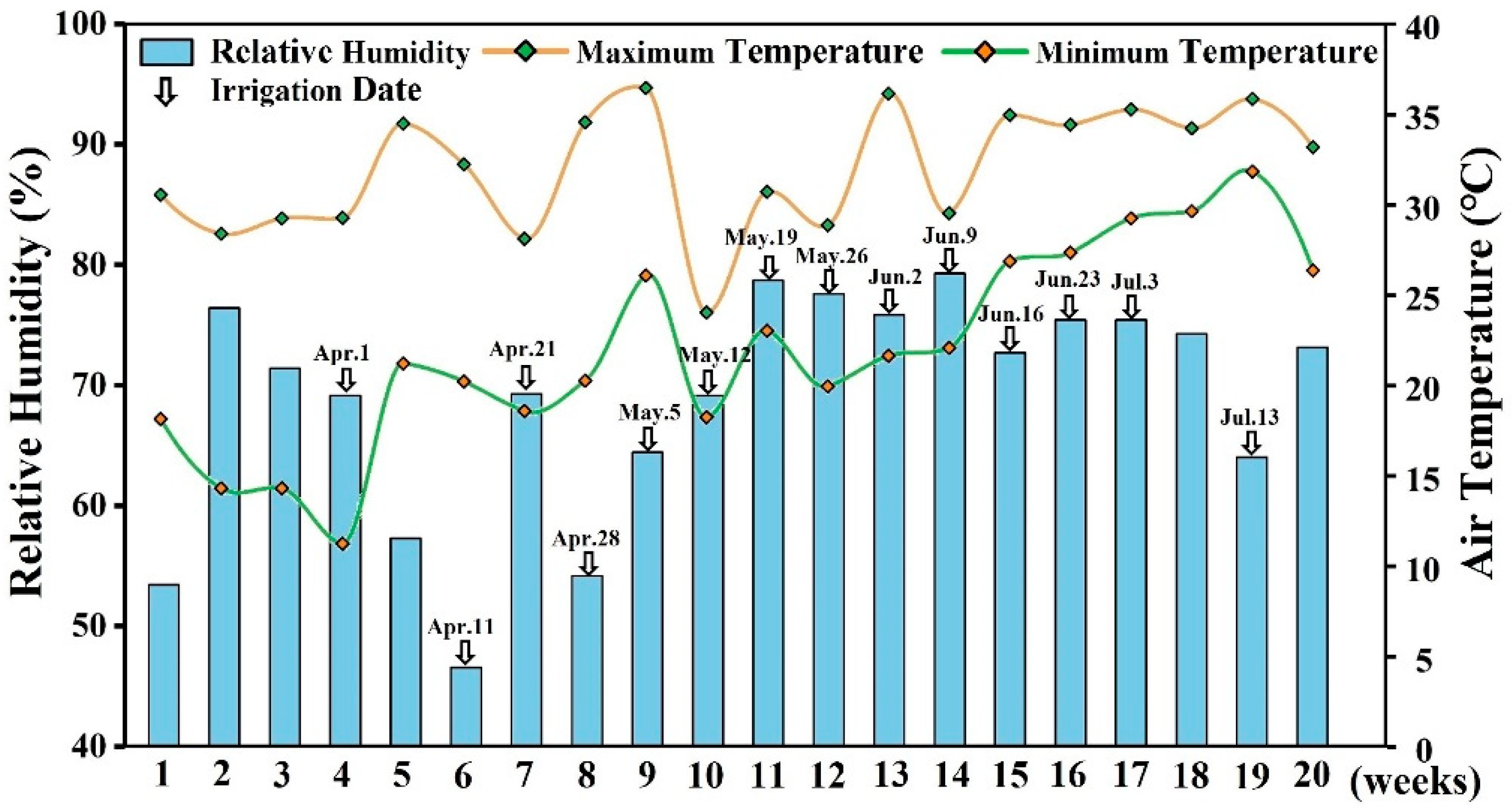
2.1. Experimental Site and Plant Material

This study was carried out on an experimental field of Yangzhou University (32°23′ N, 119°25′ E) in Yangzhou, China. Soil texture in the study area was sandy loam. The volumetric water content (VWC) of field capacity and permanent wilting point were 18% and 8% along the soil layers, respectively. The average soil pH was 7.1. Other detailed soil characteristics are shown in Table S1 (Supplementary Materials (SM)). This experimental area is located in a subtropical monsoon climate with 3.5 m altitude and 1030 mm annual average precipitation. Annual average temperature and sunshine are 15 °C and 2177 h, respectively. The tomato cultivar (Jin Guan No. 1), which is a mid-early type cultivar with good potential soluble solids content (average: 4.5%) and a high level of fruit weight (average: 200 g), was employed in the field experiment.

2.2. Field Management

A semicircular shaped greenhouse, which was covered with plastic film and oriented in a north–south direction, was employed for the tomato experiment. Six-week-old seedlings were transplanted in the early spring (13 March 2013), and the final harvest date was 13 July 2013. The row spacing was set to 0.6 m, and the distance between plants was 0.3 m with a plant density of 2.8 plant/m². The inline emitter of the drip system discharged 3 L/h with the distance being 0.3 m apart. The layout of installed drip system and experimental design in the greenhouse are illustrated in Figure S1 in the SM.

Five different DI scenarios were designed in the field experiment according to the actual percentage of tomato ET in previous studies [16]. The ET values were determined by the Penman-Monteith equation [28]. The five levels of irrigation rates at 25% ET interval were conducted as 50% ET, 75% ET, 100% ET, 125% ET, and 150% ET, which were named ET50, ET75, ET100, ET125, ET150, respectively. All scenarios were set up in a randomized block designed with three replicates (shown in Figure S1). The irrigation events were conducted at an interval of 7–10 days during the growing season. Details of the irrigation rates and scheduling are shown in Table S2 in the SM. Soluble NPK fertilizers (10-5-5) were applied at the crop root zone of each scenario by the drip irrigation system. The N fertilizer rate in each scenario was set to 200 kg/ha according to the local recommended dose for tomato requirements.

In each scenario, leaf area index (LAI) was measured by using an LAI-3000A Plant Canopy Analyzer (Li-Cor, Inc, Lincoln, NE, USA). Plant height was measured with a tape measure, and samples were randomly collected at intervals of 10 days. Over 9 plant samples in each scenario were randomly selected at the harvest date, and they were weighed to obtain biomass and yield. Soil samples were collected from four soil layers (viz., 0–5, 5–15, 15–35 and 35–55 cm) within 2–3 days after each irrigation event. Then, soil volumetric water content (VWC) of each sample was measured according to the gravitational method. The meteorological information was measured by using the sensors in the greenhouse, similar to our previous study [29]. The maximum/minimum temperature and relative humidity during the growing season are shown in Figure 1.

2.3. RZ-SHAW Overview, Model Input and Calibration

2.3.1. Model Description

The RZ-SHAW model (version 4.2) is a process-oriented finite irrigation strategy evaluation model on frequent spatiotemporal measurements of driving variables [29]. This model is a coupling of the Root Zone Water Quality Model 2 (RZWQM2) and the Simultaneous Heat and Water (SHAW) sub-model [30]. In RZWQM2, unsaturated soil water flow and redistribution were modeled using one-dimensional Richards’ equation. The modified Brooks-Corey equation was used to describe the soil water retention curve [31]. The potential demand was calculated using the extended Shuttleworth–Wallace ET model [23]. The DSSAT crop model was incorporated into RZWQM2 to provide a detailed biophysical crop model to better simulate tomato growth processes, e.g., phenological stage, LAI, plant height, biomass and yield [32]. Water absorption by plants followed the Nimah-Hanks equation [33]. Then, the RZWQM2 sub-model provided these soil-water-plant parameters at each time step to the SHAW sub-model. In turn, the SHAW sub-model fed back to RZWQM with the modifications of soil-water-plant parameters, e.g., VWC, soil temperature, soil ET, root distribution, crop growth parameters [34]. For plastic film mulching conditions, the SHAW sub-model ignored head transfer due to evaporation and condensation between the cover and the soil surface, and assumed that soil moisture evaporated only from the non-cover area [35].

2.3.2. Model Input, Calibration and Validation

The model was calibrated by using the measured data of the full irrigation (viz., ET100) in terms of tomato growth parameters (i.e., tomato LAI, plant height, biomass and yield) and soil water (i.e., VWC). Then, the model was validated by using the data from the other scenarios (viz., ET50, ET75, ET125, and ET150).

The daily weather data for running the model were obtained from the measured values, including maximum and minimum air temperature, relative humidity, solar shortwave radiation, wind speed, and precipitation. Natural precipitation and wind speed were intercepted in the greenhouse production system. Thus, the precipitation and wind speed were set to zero in this model. Soil profile in the model was divided into 7 horizons of 0–5, 5–15, 15–35, 35–55, 55–75, 75–100, 100–150 cm. The soil texture, bulk density, and organic matter content along the horizons were set to the measured values. The soil hydraulic parameters referred to our previous study [29] and were slightly modified by the VWC calibration, which is present in

Table 1. Soil hydraulic parameters along the soil layers in the RZ-SHAW model at the experimental sites.

Depth (cm)	BD (mg m−3)	Pb (cm)	θs (cm3 cm−3)	θr (cm3 cm−3)	Ksat (cm/h)	λ	Soil Root Growth Factors
0–5	1.322	−8.96	0.37	0.10	3.15	0.17	1.00
5–15	1.322	−18.53	0.34	0.13	3.22	0.32	0.90
15–35	1.402	−8.16	0.43	0.15	3.46	0.37	0.70
35–55	1.402	−23.89	0.41	0.11	1.81	0.16	0.54
55–75	1.402	−5.53	0.31	0.10	2.83	0.15	0.30
75–100	1.550	−5.53	0.31	0.10	2.83	0.15	0.20
100–150	1.550	−16.68	0.40	0.07	3.02	0.30	0.05

Note: BD: bulk density, P_b: bubbling pressure, θ_s: saturated water content, θ_r: residual water content, K_sat: saturated hydraulic conductivity, λ: pore size distribution index. Other required parameters for running the model were the default constraints.

. The faction plastic cover in the SHAW sub-model was set to 0.7, according to the actual cover ratio of plastic mulch in the greenhouse. Moreover, the plant parameters of the DSSAT sub-model were manually calibrated against observed LAI, plant height, biomass, and yield, which are detailed in

Table 2. Calibrated DSSAT parameters for tomato cultivar (Jin Guan No. 1).

Parameter	Description	Value
CSDL	Critical Short-Day Length below which reproductive development progresses with no daylength effect (for short day plants) (hour)	12.0
PPSEN	Slope of the relative response of development to photoperiod with time (positive for short day plants) (1/h)	0.0
EM-FL	Time between plant emergence and flower appearance (R1) (photothermal days)	20.0
FL-SH	Time between first flower and first pod (R3) (photothermal days)	9.5
FL-SD	Time between first flower and first seed (R5) (photothermal days)	19.8
SD-PM	Time between first seed (R5) and physiological maturity (R7) (photothermal days)	49.0
FL-LF	Time between first flower (R1) and end of leaf expansion (photothermal days)	50.3
LFMAX	Maximum leaf photosynthesis rate at 30 C, 350 vpm CO2, and high light (mg CO2/m2-s)	1.1
SLAVR	Specific leaf area of cultivar under standard growth conditions (cm2/g)	357.7
SIZLF	Maximum size of full leaf (three leaflets) (cm2)	333.1
XFRT	Maximum fraction of daily growth that is partitioned to seed and shell	0.69
WTPSD	Maximum weight per seed (g)	0.004
SFDUR	Seed filling duration for pod cohort at standard growth conditions (photothermal days)	30.0
SDPDV	Average seed per pod under standard growing conditions (#/pod)	300.0
PODUR	Time required for cultivar to reach final pod load under optimal conditions (photothermal days)	67.9

.

2.4. Statistical Analysis

The performance of simulations and observations in terms of LAI, plant height and VWC, was evaluated using four statistical criteria, i.e., relative root mean square error (RRMSE), the percent bias (PBIAS), index of agreement (IoA), and determination of coefficient (R²). Model performance was considered acceptable if −30% < RRMSE < 30%, −15% < PBIAS < 15%, IoA > 0.75 and R² > 0.5. Relative error (RE) was applied to assess the simulated performance of biomass and yield. Meanwhile, analysis of variance (ANOVA) of data from the five scenarios was performed to assess effects of DI management with a significance level of 0.05. The calculation formulae of statistical criteria are shown below:

$$\mathrm{RRMSE}=\sqrt{\frac{1}{n}{\displaystyle \sum _{i=1}^n{\left(O_i-P_i\right)}^2}}/\overline{O}$$

(1)

$$\mathrm{PBIAS}={\displaystyle \sum _{i=1}^n\left(O_i-P_i\right)}/{\displaystyle \sum _{i=1}^n{O}_i}$$

(2)

$$\mathrm{IoA}=1-{\displaystyle \sum _{i=1}^n{\left(O_i-P_i\right)}^2}/{\displaystyle \sum _{i=1}^n{\left(\left|P_i-\overline{P}\right|+\left|O_i-\overline{O}\right|\right)}^2}$$

(3)

$${\mathrm{R}}^{{}^2}={\left[{\displaystyle \sum _{i=1}^n\left(O_i-\overline{O}\right)\left(P_i-\overline{P}\right)}\right]}^2/{\displaystyle \sum _{i=1}^n{\left(O_i-\overline{O}\right)}^2{\displaystyle \sum _{i=1}^n{\left(P_i-\overline{P}\right)}^2}}$$

(4)

$$\mathrm{RE}=\left(P_i-O_i\right)/O_i$$

(5)

where O_i and P_i represent the observed and simulated values, respectively. $\overline{O}$ and $\overline{P}$ represent the mean observed and simulated values, respectively. The value n represents the number of observations.

2.5. Quantifying the Effects of Deficit Irrigation Levels using Calibrated RZ-SHAW

By using the calibrated RZ-SHAW model, the water deficiency degrees of five experimental scenarios were estimated by plant water stress factor (PWSF) [35]. The PWSF is the indicator of water deficiency by calculating the ratio of DSSAT of root water absorption to ET [36], which ranges from 1 for no stress to 0 for complete stress.

In order to further explore optimal DI management, the quantification of splitting irrigation rate impact on yield, WP and PWSF was determined by using calibrated RZ-SHAW. A total of 45 scenarios were investigated with different DI levels from 0% ET to 225% ET at 5% ET interval. The WP in these DI scenarios were calculated as:

$$\mathrm{WP}=\mathrm{Yield}/\left(\mathrm{IM}+\Delta \mathrm{SW}\right)$$

(6)

where WP (kg/(ha·mm)) is the water productivity. IM (mm) is the total irrigation amount. ∆SW (mm) is the difference of water stored in the soil between planting and harvest.

3. Results

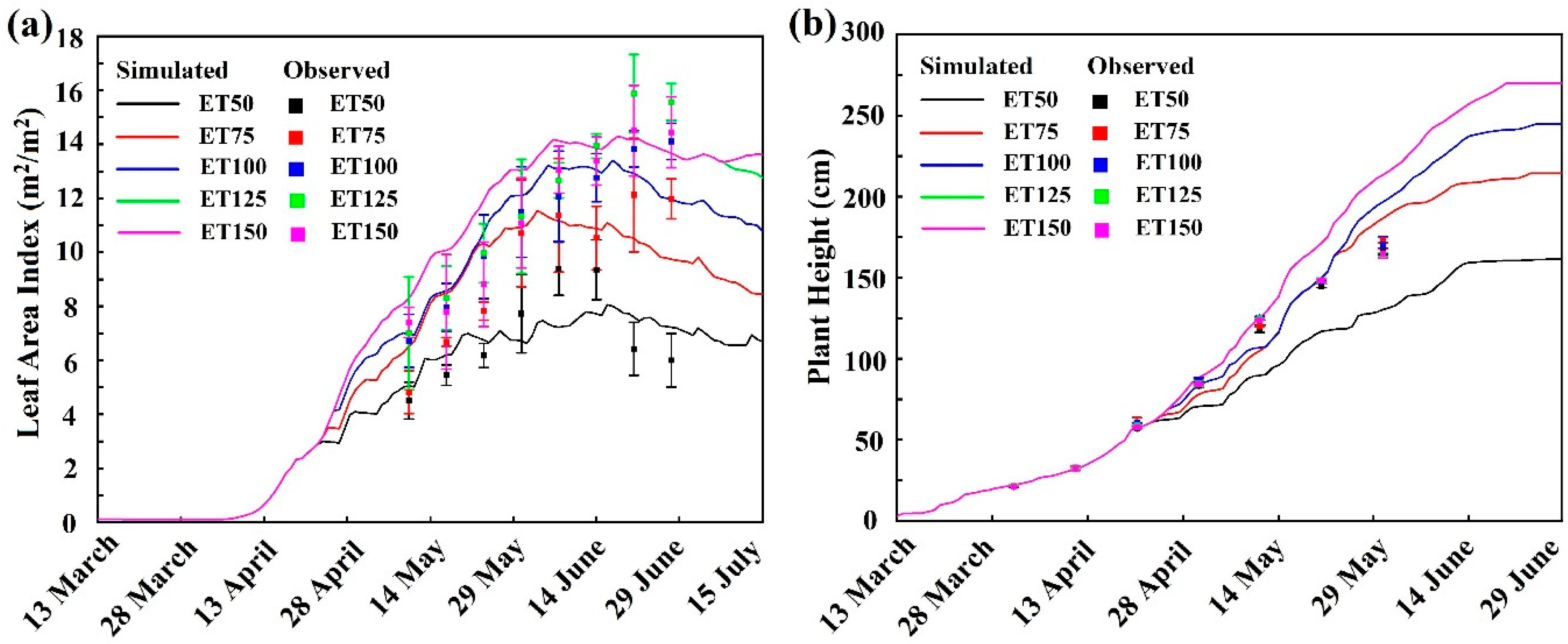
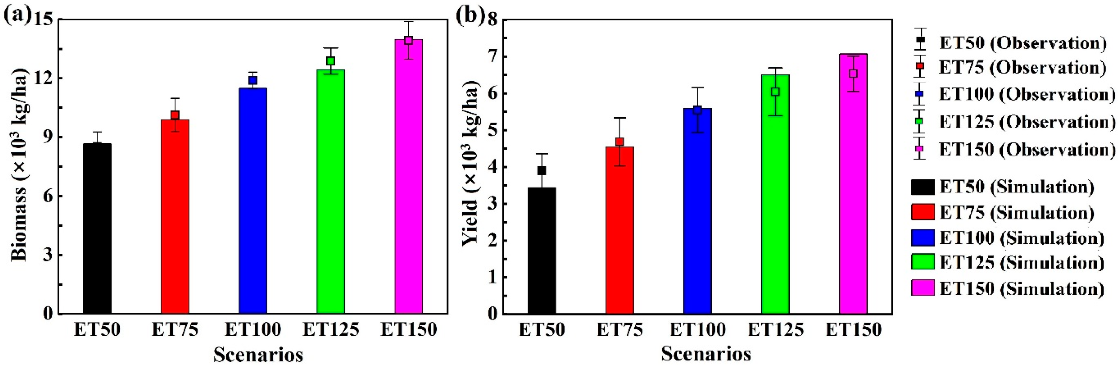
3.1. Simulations of Tomato Growth Parameters

Statistical analyses indicated that the simulated LAI was in good agreement with the observed data, shown in

Table 3. Statistical criteria results obtained by comparing the observed and simulated LAI (cm²/cm²), plant height, biomass and yield in each scenario.

Scenarios	LAI						Plant Height						Biomass	Yield
	ObLAI	SimLAI	RRMSE	PBIAS	IoA	R2	ObPH	SimPH	RRMSE	PBIAS	IoA	R2	RE	RE
ET50	6.9	6.8	18.1%	1.0%	0.73	0.70	89.0	74.1	23.5%	16.7%	0.95	1.00	8.7%	12.1%
ET75	9.5	9.8	16.7%	−3.4%	0.84	0.83	91.5	90.1	9.1%	1.6%	0.99	0.99	8.3%	14.0%
ET100	11.1	11.2	9.2%	−0.8%	0.95	0.92	92.1	92.6	13.4%	−0.5%	0.99	0.98	3.5%	11.3%
ET125	11.8	12.4	13.4%	−4.8%	0.90	0.91	90.7	101.3	22.7%	−11.7%	0.97	0.99	5.2%	10.8%
ET150	11.3	12.4	14.5%	−9.6%	0.88	0.91	90.4	101.3	22.6%	−12.1%	0.97	0.99	6.9%	7.0%

Note: LAI: leaf area index (m²/m²). Ob_LAI and Ob_PH: the mean observed value of LAI and plant height, respectively; Sim_LAI and Sim_PH: the mean simulated value of LAI and plant height, respectively. The ET100 scenario was the calibration phase. The remaining four scenarios (i.e., ET50, ET75, ET125, and ET150) were the validation phase. The statistical criteria were calculated by Equations (1)–(5).

. The RRMSE, PBIAS, IoA and R² between the observed and simulated LAI were 14.4% ± 3.4%, −3.5% ± 4.1%, 0.86 ± 0.08 and 0.85 ± 0.09, respectively. As shown in Figure 2a, the LAI rose significantly with irrigation rates (p < 0.05). The LAI values in each sampling event showed a strongly positive correlation with the percentage of ET, and the Pearson correlation coefficients (r) were 0.94 ± 0.02 for simulation and 0.86 ± 0.08 for observation, respectively. This phenomenon was because adequate water promoted chlorophyll synthesis and delayed the fading of crop leaves [37]. Meanwhile, there was little difference between the ET125 and ET150 in both simulation and observation. This was explained by the fact that the photosynthetic rate approached a saturation plateau when soil water exceeded the threshold [38].

In contrast to the LAI, simulated plant height was in better agreement with the observation with the IoA > 0.95 and R² > 0.98, respectively (Table 3). It was found that higher irrigation rates tended to increase simulated plant height (Figure 2b). The mean simulated values of plant height (Sim_PH) increased from 74.1 cm for ET50 to 101.3 cm for ET150, respectively. However, the observed plant height among the five scenarios had no significant difference (p > 0.05). A similar phenomenon was observed in a previous study [29].

The biomass and yield were also well-simulated by RZ-SHAW. The RE values were in the range of 3.5–8.7% for biomass and 7.0–14.0% for yield, respectively (Table 3). As shown in Figure 3a,b, both biomass and yield increased by 1.1–1.3 times for every 25% increase in irrigation rates, i.e., ET50 < ET75 < ET100 < ET125 < ET150. The simulated biomass and yield were 8672 and 3429 kg/ha for ET50, respectively, and were 13,982 and 7069 kg/ha for ET150, respectively. Some previous studies also showed that the tomato yield increased 1.1–1.3 times for every 25% increase in irrigation rates [39,40], which were similar to our results. The higher biomass and yield in the scenarios with high DI levels were attributed to the higher net photosynthetic rates and transpiration rates, which led to a rise in biomass and yield [41].

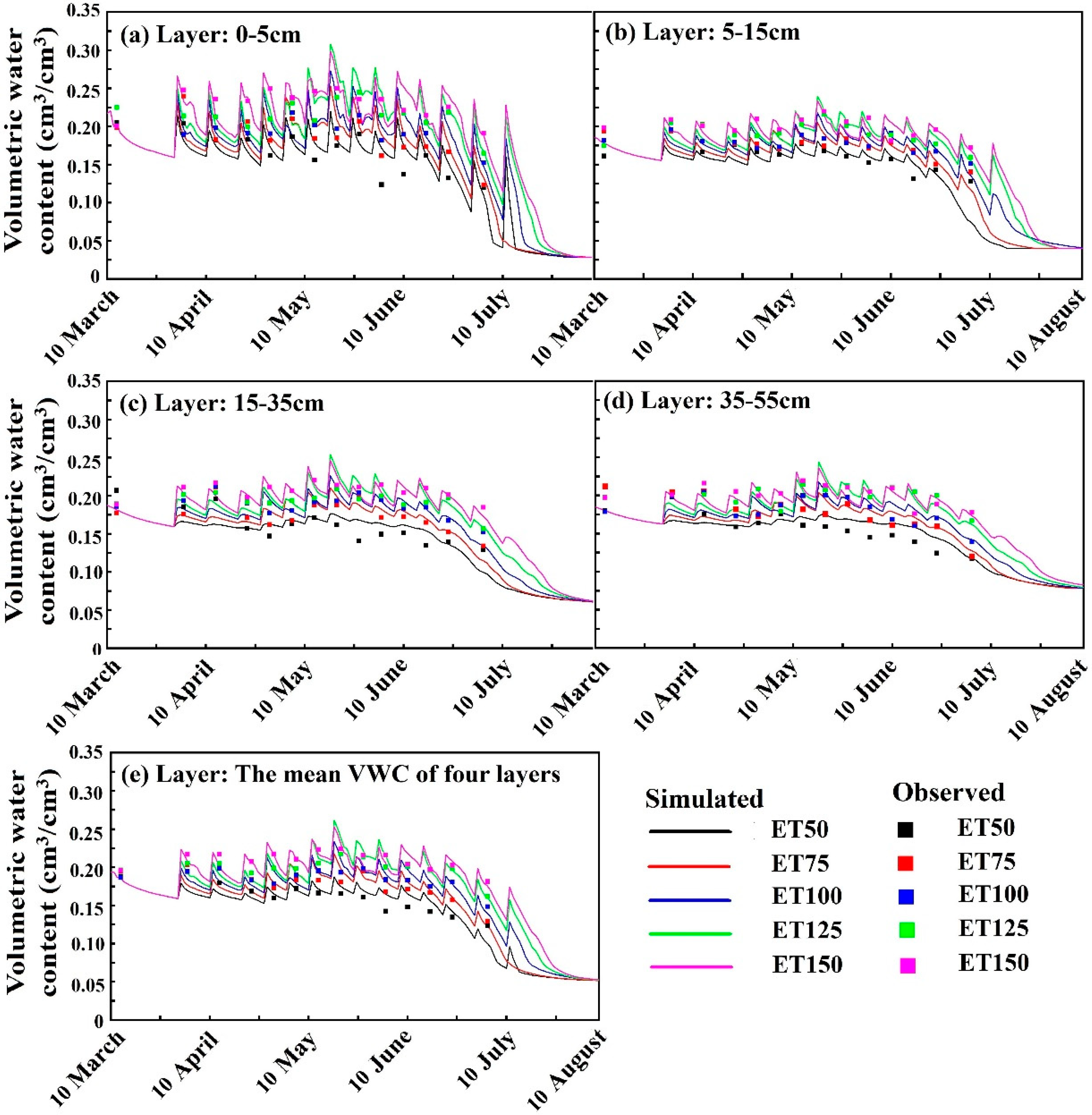
3.2. Simulations for Soil Water

The statistical criteria between observed and simulated VWC are presented in

Table 4. Statistical criteria results obtained by comparing the observed and simulated VWC (cm³/cm³) along the soil layers in each scenario.

Depth (cm)	ET50 (Validation)						ET75 (Validation)
	ObVWC	SimVWC	RRMSE	PBIAS	IoA	R2	ObVWC	SimVWC	RRMSE	PBIAS	IoA	R2
0–5	0.166	0.171	12.4%	−3.2%	0.79	0.70	0.185	0.187	11.0%	−0.8%	0.76	0.64
5–15	0.161	0.156	11.9%	3.1%	0.74	0.65	0.176	0.179	8.5%	2.9%	0.76	0.64
15–35	0.160	0.159	11.7%	0.3%	0.77	0.61	0.174	0.175	8.9%	−0.3%	0.82	0.68
35–55	0.157	0.162	9.5%	−3.2%	0.81	0.75	0.177	0.175	10.0%	1.3%	0.76	0.64
Mean (0–55)	0.161	0.162	8.7%	−0.7%	0.86	0.75	0.178	0.177	7.7%	0.8%	0.85	0.72
Depth (cm)	ET100 (Calibration)						ET125 (Validation)
0–5	0.195	0.198	8.5%	−1.6%	0.74	0.56	0.215	0.221	9.4%	−2.9%	0.79	0.72
5–15	0.177	0.179	5.9%	−0.7%	0.81	0.69	0.191	0.191	5.7%	−0.3%	0.86	0.74
15–35	0.187	0.184	7.1%	1.4%	0.80	0.67	0.193	0.198	7.1%	−2.3%	0.77	0.69
35–55	0.181	0.183	7.1%	−0.6%	0.82	0.70	0.200	0.194	5.7%	2.8%	0.82	0.76
Mean (0–55)	0.185	0.186	5.5%	−0.4%	0.86	0.76	0.200	0.201	5.6%	−0.7%	0.86	0.83
Depth (cm)	ET150 (Validation)
0–5	0.230	0.230	5.9%	0.3%	0.86	0.73
5–15	0.200	0.196	5.6%	1.9%	0.74	0.59
15–35	0.207	0.203	4.1%	1.7%	0.85	0.79
35–55	0.202	0.199	5.7%	1.5%	0.72	0.57
Mean (0–55)	0.210	0.207	4.3%	1.3%	0.86	0.76

Note: VWC: soil volumetric water content (cm³/cm³), Ob_VWC and Sim_VWC: the observed and simulated mean value of VWC, respectively. The statistical criteria were calculated by Equations (1)–(4).

. The model satisfactorily predicted VWC at all soil layers with RRMSE <12.4%, PBIAS within ±3.2%, IoA > 0.72 and R² > 0.56, respectively. The mean observed and simulated VWC (0–55 cm) increased from 0.161 and 0.162 cm³/cm³ for ET50 to 0.210 and 0.207 cm³/cm³ for ET150, respectively.

As shown in Figure 4a–e, both observed and simulated VWCs were obviously increased with the DI levels (p < 0.01), and each sharper peak occurred 1 day after irrigation events. A similar phenomenon was also observed in previous studies [7,29]. This was because without recharge from rainfall and groundwater, the irrigation events were the main source of soil moisture in the greenhouse [34]. Meanwhile, the peak VWC values of the upper layers were sharper than the lower layers. Chen et al. [42] also reported that the simulated VWC showed a declining trend along with the soil layers in a two-year field experiment. This was due to the stronger water-holding capacity in the upper layers, which was caused by smaller bulk density and larger soil porosity in surface soil than the deeper soil [43,44].

4. Discussion

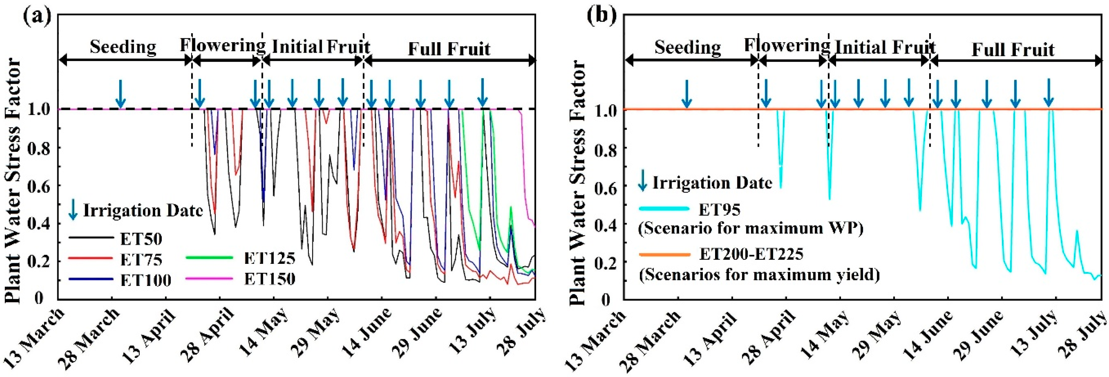
4.1. Simulated Plant Water Stress in Experimental Scenarios

The plant water stress factor (PWSF) is an important water deficit indicator, and the occurrence of water stress is the main reason for biomass and yield reduction in the model [36,45]. Tomato growth would suffer from more severe water stress when PWSF approached zero. As shown in Figure 5a, there was a negative correlation between PWSF values and irrigation rates (p < 0.01). The mean PWSFs were 0.98 for ET150, 0.91 for ET125, 0.84 for ET100, 0.75 for ET75 and 0.69 for ET50, respectively. This was the main reason for the biomass and yield reduction in the scenarios with low DI levels (Figure 3). Meanwhile, water stress would reappear soon when the irrigation rates were deficient, e.g., ET50 and ET75. It was found that the water stress of tomatoes mainly appeared in initial and full fruit stages from 10 May to 28 July. This might be due to the larger water consumption in the late crop growth stages, wherein large amounts of auxin and cytokinin were secreted to stimulate fruit enlargement [46,47]. The results indicated that the PWSF, as simulated using RZ-SHAW, could potentially be used to trigger irrigation, thereby informing the development of optimal DI management for improving yield and WP.

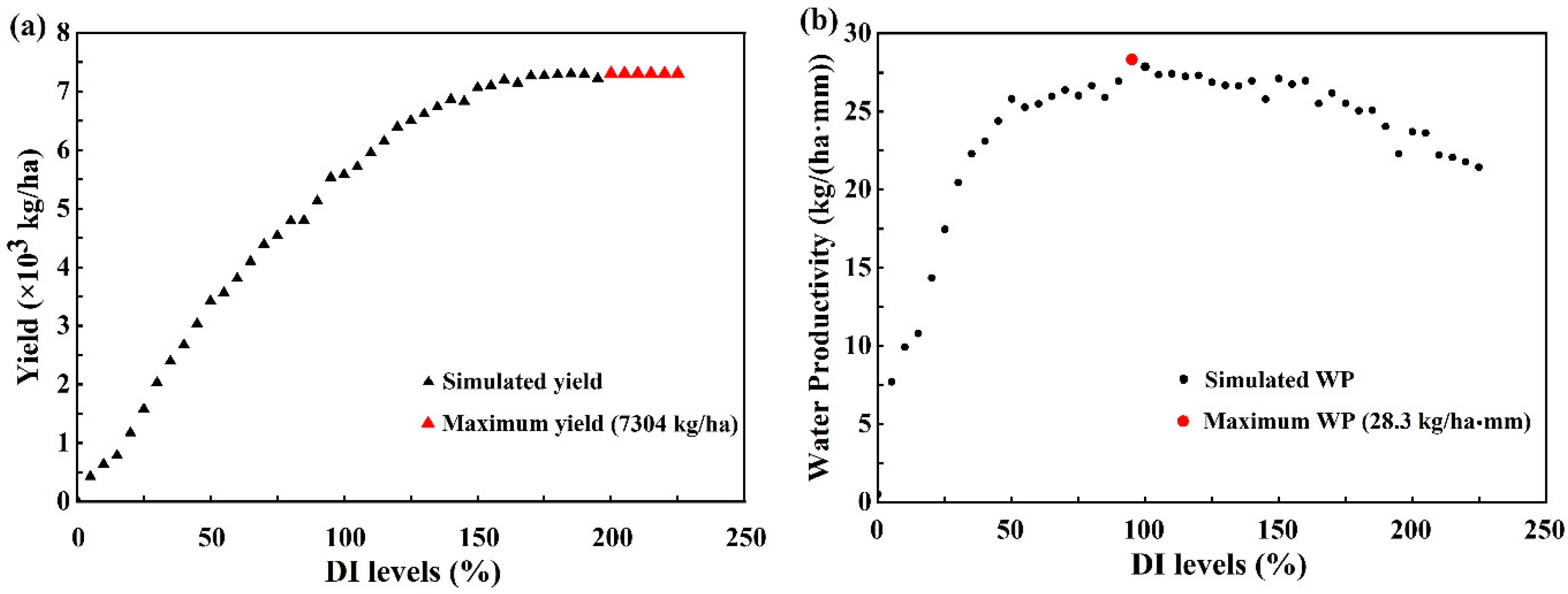
4.2. Optimizing Deficit Irrigation Management for Maximizing Yield and Water Productivity

To obtain the optimum DI management for improving yield and WP, a series of DI levels was simulated using the calibrated model. The simulated yield rapidly increased with the DI levels when the levels were below ET150, shown in Figure 6a. The yield increased from 24 kg/ha for ET0 to 7069 kg/ha for ET150, respectively. Then, the yield increased slightly with the DI levels from ET150 to ET200 scenario, and the yield merely increased by 3.2%. The irrigation approach suggested that applying 32.30 cm water (Table S2 in the SM) to the tomato cultivar (Jin Guan No. 1) over the growing season allowed the crop to achieve its highest yield potential (7304 kg/ha). When the DI levels exceeded ET200, the potential yield remained unchanged, which was because no water stress occurred in the ET200-225 scenarios through the whole phenological stages, shown in Figure 5b. It also indicated the water stress-based method was an efficient way to schedule high-yield. Moreover, among the mainstream tomato cultivars in the world, the mean tomato yield was reported to be about 6000 kg/ha [16]. The maximum yield of tomato cultivar (Jin Guan No. 1) in this study was higher than this mean value, which showed a promising high-yield cultivar.

There was a significantly increased tendency of WP from ET0 to ET95 (Figure 6b). This was because the WP was the ratio of yield to water consumption (Equation (6)), and the yield increased much faster than the increased irrigation rates before the ET95 scenario. This result agreed with Fang et al. [48] and Liu et al. [49]. The maximum WP appeared in the ET95 scenario, and the value was 28.3 kg/(ha·mm). The WPs in ET95 were 8.8%, 8.1%, 1.4%, 4.9% and 4.2% higher than ET50, ET75, ET100, ET125 and ET150 in the experiment, respectively. As shown in Figure 5b, the mean PWSF in ET95 was 0.82, indicating that slight water stress contributed to an increase in WP. The corresponding irrigation rate was 15.67 cm (Table S2 in the SM), which was only 48.5% of the highest yield scenario in ET200. Meanwhile, the simulated yield value was 5535 kg/ha, which had 24% yield sacrifice compared to ET200, due to insufficient irrigation. Moreover, when the irrigation rates were higher than ET95, the WP showed a declining tendency from 28.3 kg/(ha·mm) for ET95 to 21.4 kg/(ha·mm) for ET225. This could be attributed to the stable tendency of yield from ET95 to ET225 (Figure 6b), in which increased irrigation rates played the dominant role in the change in WP. Compared to previous studies, the optimal DI levels for max WP appeared in the range of 50–100% ET [10,11,12,13,14]. The optimal DI scenario in this study (i.e., ET95) was also in this range. Meanwhile, it was reported that the optimal WP values for tomato production generally fluctuated within the range of 18.2 to 27.6 kg/(ha·mm) [50,51]. The optimal WP in this study (i.e., 28.3 kg/(ha·mm)) was slightly higher than previous reports, which might have resulted from more appropriate temperature at the reproductive phase in the greenhouse experiment. The early sown tomatoes in this study (13 March) escaped the risk of terminal heat stress and, thus, produced better yield [52]. The results showed that yield and WP using the water-stress method could be improved by optimizing DI levels, which could be provided as a reference for local farmers and policymakers.

5. Conclusions

DI management is widely recommended around the world to improve tomato yield and WP. In this study, the RZ-SHAW proved to be a promising tool in evaluating the effects of DI strategies on tomato LAI, plant height, biomass, yield, and soil water along the layers in a drip-irrigated, plastic film mulching, greenhouse field. Plant water stress proved to be a key factor affecting the tomato LAI, biomass and yield, especially in initial and full fruit stages. Based on the water stress-based method, the optimal DI levels for maximizing yield and WP could be achieved by applying the calibrated model. The maximum yield appeared in abundant irrigation input without the occurrence of plant water stress. The maximum WP appeared under moderate DI levels with some sacrifice in yield. The results provided a water stress-based irrigation scheduling method to derive optimum DI management for improving tomato yield and WP by using RZ-SHAW. In addition, the potential for adaptation of other influencing factors for simulation of tomato production in RZ-SHAW across soil types and climate changes needs to be verified in further studies.

References

1. Barros, L.; Duenas, M.; Pinela, J.; Carvalho, A.M.; Buelga, C.S.; Ferreira, I.C.F.R. Characterization and quantification of phenolic compounds in four tomato (Lycopersicon esculentum L.) farmers’ varieties in northeastern portugal homegardens. Plant Food Hum. Nutr. 2012, 67, 229–234. [Google Scholar] [CrossRef] [PubMed]
2. Food and Agriculture Organization. FAOSTAT. Area Harvested/Production/Yield Quantities of Tomatoes in World + (Total). Available online: https://www.fao.org/faostat/en/#data/QCL (accessed on 1 August 2022).
3. Geng, G.; Wu, J.; Wang, Q.; Lei, T.; He, B.; Li, X.; Mo, X.; Luo, H.; Zhou, H.; Liu, D. Agricultural drought hazard analysis during 1980–2008: A global perspective. Int. J. Climatol. 2016, 36, 389–399. [Google Scholar] [CrossRef]
4. Francesca, S.; Cirillo, V.; Raimondi, G.; Maggio, A.; Barone, A. A novel protein hydrolysate-based biostimulant improves tomato performances under drought stress. Plants 2021, 10, 783. [Google Scholar] [CrossRef] [PubMed]
5. Antolinos, V.; Sanchez-Martinez, M.J.; Maestre-Valero, J.E.; Lopez-Gomez, A.; Martinez-Hernandez, G.B. Effects of irrigation with desalinated seawater and hydroponic system on tomato quality. Water 2020, 12, 518. [Google Scholar] [CrossRef]
6. Khapte, P.S.; Kumar, P.; Burman, U.; Kumar, P. Deficit irrigation in tomato: Agronomical and physio-biochemical implications. Sci. Hortic. 2019, 248, 256–264. [Google Scholar] [CrossRef]
7. Cheng, H.; Shu, K.; Zhu, T.; Wang, L.; Liu, X.; Cai, W.; Qi, Z.; Feng, S. Effects of alternate wetting and drying irrigation on yield, water and nitrogen use, and greenhouse gas emissions in rice paddy fields. J. Clean. Prod. 2022, 349, 131487. [Google Scholar] [CrossRef]
8. Wang, D.; Zhang, H.; Gartung, J. Long-term productivity of early season peach trees under different irrigation methods and postharvest deficit irrigation. Agric. Water Manag. 2020, 230, 105940. [Google Scholar] [CrossRef]
9. Cheng, M.; Wang, H.; Fan, J.; Fan, J.; Liao, Z.; Zhang, F.; Wang, Y. A global meta-analysis of yield and water use efficiency of crops, vegetables and fruits under full, deficit, alternate partial root-zone irrigation. Agric. Water Manag. 2021, 248, 106771. [Google Scholar] [CrossRef]
10. Patanè, C.; Tringali, S.; Sortino, O. Effects of deficit irrigation on biomass, yield, water productivity and fruit quality of processing tomato under semi-arid mediterranean climate conditions. Sci. Hortic. 2011, 129, 590–596. [Google Scholar] [CrossRef]
11. Mahmoud, M.M.A.; Fayad, A.M. The effect of deficit irrigation, partial root drying and mulching on tomato yield, and water and energy saving*. Irrig. Drain. 2022, 71, 295–309. [Google Scholar] [CrossRef]
12. Wu, Y.; Yan, S.; Fan, J.; Zhang, F.; Zhao, W.; Zheng, J.; Guo, J.; Xiang, Y.; Wu, L. Combined effects of irrigation level and fertilization practice on yield, economic benefit and water-nitrogen use efficiency of drip-irrigated greenhouse tomato. Agric. Water Manag. 2022, 262, 107401. [Google Scholar] [CrossRef]
13. Elnemr, M. Integration of subsurface irrigation and organic mulching with deficit irrigation to increase water use efficiency of drip irrigation. Inmateh-Agric. Eng. 2021, 64, 215–226. [Google Scholar]
14. Jensen, C.R.; Battilani, A.; Plauborg, F.; Psarras, G.; Chartzoulakis, K.; Janowiak, F.; Stikic, R.; Jovanovic, Z.; Li, G.T.; Qi, X.B.; et al. Deficit irrigation based on drought tolerance and root signalling in potatoes and tomatoes. Agric. Water Manag. 2010, 98, 403–413. [Google Scholar] [CrossRef]
15. Stoleru, V.; Inculet, S.C.; Mihalache, G.; Cojocaru, A.; Teliban, G.C.; Caruso, G. Yield and nutritional response of greenhouse grown tomato cultivars to sustainable fertilization and irrigation management. Plants 2020, 9, 1053. [Google Scholar] [CrossRef] [PubMed]
16. Chand, J.B.; Hewa, G.; Hassanli, A.; Myers, B. Deficit irrigation on tomato production in a greenhouse environment: A review. J. Irrig. Drain. Eng. 2021, 147, 04020041. [Google Scholar] [CrossRef]
17. Hemming, S.; de Zwart, F.; Elings, A.; Petropoulou, A.; Righini, I. Cherry tomato production in intelligent greenhouses-sensors and ai for control of climate, irrigation, crop yield, and quality. Sensors 2020, 20, 6430. [Google Scholar] [CrossRef]
18. Huang, W.; Zhu, Y.L.; Wang, D.B.; Wu, N. Assessment on the coupling effects of drip irrigation and se-enriched organic fertilization in tomato based on improved entropy weight coefficient model. Bull. Environ. Contam. Toxicol. 2021, 106, 884–891. [Google Scholar] [CrossRef]
19. Zhou, H.; Chen, J.; Wang, F.; Li, X.; Genard, M.; Kang, S. An integrated irrigation strategy for water-saving and quality-improving of cash crops: Theory and practice in China. Agric. Water Manag. 2020, 241, 106331. [Google Scholar] [CrossRef]
20. Chen, N.; Li, X.; Shi, H.; Hu, Q.; Zhang, Y.; Hou, C.; Liu, Y. Modeling evapotranspiration and evaporation in corn/tomato intercropping ecosystem using a modified ERIN model considering plastic film mulching. Agric. Water Manag. 2022, 260, 107286. [Google Scholar] [CrossRef]
21. Ouyang, Z.; Tian, J.C.; Zhao, C.; Yan, X.F. Coupling model and optimal combination scheme of water, fertilizer, dissolved oxygen and temperature in greenhouse tomato under drip irrigation. Int. J. Agric. Biol. Eng. 2021, 14, 37–46. [Google Scholar] [CrossRef]
22. Dastranj, M.; Noshadi, M.; Sepaskhah, A.; Razzaghi, F.; Ragab, R. Soil salinity and tomato yield simulation using saltmed model in drip irrigation. J. Irrig. Drain. Eng. 2018, 144, 05017008. [Google Scholar] [CrossRef]
23. Zhang, B.; Kang, S.Z.; Zhang, L.; Tong, L.; Du, T.S.; Li, F.S.; Zhang, J.H. An evapotranspiration model for sparsely vegetated canopies under partial root-zone irrigation. Agric. For. Meteorol. 2009, 149, 2007–2011. [Google Scholar] [CrossRef]
24. Qi, Z.; Ma, L.; Bausch, W.C.; Trout, T.J.; Ahuja, L.R.; Flerchinger, G.N.; Fang, Q.X. Simulating maize production, water and surface energy balance, canopy temperature, and water stress under full and deficit irrigation. Trans. ASABE 2016, 59, 623–633. [Google Scholar]
25. Zhou, L.; Zhao, W.; He, J.; Flerchinger, G.N.; Feng, H. Simulating soil surface temperature under plastic film mulching during seedling emergence of spring maize with the RZ–SHAW and DNDC models. Trans. ASABE 2020, 197, 104517. [Google Scholar] [CrossRef]
26. Gillette, K.; Malone, R.W.; Kaspar, T.C.; Ma, L.; Parkin, T.B.; Jaynes, D.B.; Fang, Q.X.; Hatfield, J.L.; Feyereisen, G.W.; Kersebaum, K.C. N loss to drain flow and N2O emissions from a corn-soybean rotation with winter rye. Sci. Total Environ. 2018, 618, 982–997. [Google Scholar] [CrossRef] [PubMed]
27. Amatya, D.M.; Irmak, S.; Gowda, P.; Sun, G.; Nettles, J.E.; Douglas-Mankin, K.R. Ecosystem evapotranspiration: Challenges in measurements, estimates, and modeling. T. Trans. ASABE 2016, 59, 555–560. [Google Scholar]
28. Fooladmand, H.R.; Ahmadi, S.H. Monthly spatial calibration of Blaney-Criddle equation for calculating monthly ETO in south of Iran. Irrig. Drain. 2009, 58, 234–245. [Google Scholar] [CrossRef]
29. Cheng, H.; Yu, Q.; Abdalhi, M.A.M.; Li, F.; Qi, Z.; Zhu, T.; Cai, W.; Chen, X.; Feng, S. RZWQM2 simulated drip fertigation management to improve water and nitrogen use efficiency of maize in a solar greenhouse. Agriculture 2022, 12, 672. [Google Scholar] [CrossRef]
30. Fang, Q.; Ma, L.; Flerchinger, G.N.; Qi, Z.; Ahuja, L.R.; Xing, H.T.; Lie, J.; Yu, Q. Modeling evapotranspiration and energy balance in a wheat–maize cropping system using the revised RZ-SHAW model. Agric. Forest Meteorol. 2014, 194, 218–229. [Google Scholar] [CrossRef]
31. Ma, L.; Ahuja, L.R.; Nolan, B.T.; Malone, R.W.; Trout, T.J.; Qi, Z. Root Zone Water Quality Model (RZWQM2): Model use, calibration, and validation. Trans. ASABE 2012, 55, 1425–1446. [Google Scholar] [CrossRef]
32. Saseendran, S.A.; Ma, L.; Malone, R.; Heilman, P.; Ahuja, L.R.; Kanwar, R.S.; Karlen, D.L.; Hoogenboom, G. Simulating, management effects on crop production, tile drainage, and water quality using RZWQM-DSSAT. Geoderma 2007, 140, 297–309. [Google Scholar] [CrossRef]
33. Anapalli, S.S.; Ahuja, L.R.; Gowda, P.H.; Ma, L.W.; Marek, G.; Evett, S.R.; Howell, T.A. Simulation of crop evapotranspiration and crop coefficients with data in weighing lysimeters. Agric. Water Manag. 2016, 177, 274–283. [Google Scholar] [CrossRef]
34. Shrestha, D.; Jacobsen, K.; Ren, W.; Wendroth, O. Understanding soil nitrogen processes in diversified vegetable systems through agroecosystem modelling. Nutr. Cycl. Agroecosyst. 2021, 120, 49–68. [Google Scholar] [CrossRef]
35. Ma, L.; Flerchinger, G.N.; Ahuja, L.R.; Sauer, T.J.; Prueger, J.H.; Malone, R.W.; Hatfield, J.L. Simulating the surface energy balance in a soybean canopy with the SHAW and RZ-SHAW models. Trans. ASABE 2012, 55, 175–179. [Google Scholar] [CrossRef]
36. Saseendran, S.A.; Trout, T.J.; Ahuja, L.R.; Ma, L.; McMaster, G.S.; Nielsen, D.C.; Andales, A.A.; Chavez, J.L.; Ham, J. Quantifying crop water stress factors from soil water measurements in a limited irrigation experiment. Agric. Syst. 2015, 137, 191–205. [Google Scholar] [CrossRef]
37. Li, Y.; Shao, X.; Li, D.; Xiao, M.; Hu, X.; He, J. Effects of water and nitrogen coupling on growth, physiology and yield of rice. Int. J. Agric. Biol. Eng. 2019, 12, 60–66. [Google Scholar] [CrossRef]
38. Kumar, D.S.; Sharma, R.; Brar, A.S. Optimising drip irrigation and fertigation schedules for higher crop and water productivity of oilseed rape (Brassica napus L.). Irrigation Sci. 2021, 39, 535–548. [Google Scholar] [CrossRef]
39. Lipan, L.; Issa-Issa, H.; Moriana, A.; Zurita, N.M.; Galindo, A.; Martin-Palomo, M.J.; Andreu, L.; Carbonell-Barrachina, A.A.; Hernandez, F.; Corell, M. Scheduling regulated deficit irrigation with leaf water potential of cherry tomato in greenhouse and its effect on fruit quality. Agriculture 2021, 11, 669. [Google Scholar] [CrossRef]
40. Agbna, G.H.D.; She, D.L.; Liu, Z.P.; Elshaikh, N.A.; Shao, G.C.; Timm, L.C. Effects of deficit irrigation and biochar addition on the growth, yield, and quality of tomato. Sci. Hortic. 2017, 222, 90–101. [Google Scholar] [CrossRef]
41. Zhang, P.; Dai, Y.Y.; Masateru, S.; Natsumi, M.; Kengo, I. Interactions of salinity stress and flower thinning on tomato growth, yield, and water use efficiency. Commun. Soil Sci. Plan. 2017, 48, 2601–2611. [Google Scholar] [CrossRef]
42. Chen, X.; Qi, Z.; Gui, D.; Gu, Z.; Ma, L.; Zeng, F.; Li, L.; Sima, M.W. A model-based real-time decision support system for irrigation scheduling to improve water productivity. Agronomy 2019, 9, 686. [Google Scholar] [CrossRef]
43. Kisekka, I.; Schlegel, A.; Ma, L.; Gowda, P.H.; Prasad, P.V.V. Optimizing preplant irrigation for maize under limited water in the High Plains. Agric. Water Manag. 2017, 187, 154–163. [Google Scholar] [CrossRef]
44. Smagin, A.; Smagin, A.V.; Khakimova, G.M.; Khineeva, D.A.; Sadovnikova, N.B. Gravity factor of the formation of the field and capillary water capacities in soils and artificial layered soil-like bodies. Eurasian Soil. Sci. 2008, 41, 1189–1197. [Google Scholar] [CrossRef]
45. Sima, M.W.; Fang, Q.X.; Qi, Z.; Yu, Q. Direct assimilation of measured soil water content in Root Zone Water Quality Model calibration for deficit-irrigated maize. Agron. J. 2020, 112, 844–860. [Google Scholar] [CrossRef]
46. Fenn, M.A.; Giovannoni, J.J. Phytohormones in fruit development and maturation. Plant J. 2021, 105, 446–458. [Google Scholar] [CrossRef]
47. Kumari, R.; Kaur, I.; Bhatnagar, A.K. Effect of aqueous extract of Sargassum johnstonii Setchell & Gardner on growth, yield and quality of Lycopersicon esculentum Mill. J. Appl. Phycol. 2011, 23, 623–633. [Google Scholar]
48. Fang, Q.; Ma, L.; Yu, Q.; Ahuja, L.R.; Malone, R.W.; Hoogenboom, G. Irrigation strategies to improve the water use efficiency of wheat–maize double cropping systems in North China Plain. Agric. Water Manag. 2010, 97, 1165–1174. [Google Scholar] [CrossRef]
49. Liu, C.; Gu, Z.; Gui, D.; Zeng, F. Optimizing irrigation rates for cotton production in an extremely arid area using RZWQM2-simulated water stress. Trans. ASABE 2017, 60, 2041–2052. [Google Scholar] [CrossRef]
50. Bogale, A.; Nagle, M.; Latif, S.; Aguila, M.; Muller, J. Regulated deficit irrigation and partial root-zone drying irrigation impact bioactive compounds and antioxidant activity in two select tomato cultivars. Sci. Hortic. 2016, 213, 115–124. [Google Scholar] [CrossRef]
51. Nuruddin, M.M.; Madramootoo, C.A.; Dodds, G.T. Effects of water stress at different growth stages on greenhouse tomato yield and quality. Hortscience 2003, 38, 1389–1393. [Google Scholar] [CrossRef]
52. Bana, R.S.; Bamboriya, S.D.; Padaria, R.N.; Dhakar, R.K.; Khaswan, S.L.; Choudhary, R.L.; Bamboriya, J.S. Planting period effects on wheat productivity and water footprints: Insights through adaptive trials and APSIM simulations. Agronomy 2022, 12, 226. [Google Scholar] [CrossRef]
Figure 1. Relative humidity (%), maximum/minimum temperature (°C), irrigation dates in the experimental period from 6 March to 24 July.
Agriculture 12 01253 g001
Figure 2. The simulated versus observed leaf area index (LAI) (a) and plant height (b) under five deficit irrigation (DI) scenarios. The error bars were 2.4–29.8% for observed LAI and 0.1–5.8% for observed plant height, respectively.
Agriculture 12 01253 g002
Figure 3. The simulated and observed biomass (a) and yield (b) under five scenarios. The error bars of the observed biomass and yield were in the range of 3.5–8.7% and 7.0–14.0% respectively.
Agriculture 12 01253 g003
Figure 4. Observed versus simulated volumetric water content (VWC, cm3/cm3) for each scenario along the soil layers of 0–5 cm (a), 5–15 cm (b), 15–35 cm (c), 35–55 cm (d) and the mean VWC of the four layers (e).
Agriculture 12 01253 g004
Figure 5. The simulated plant water stress factor (PWSF) in the five experimental DI scenarios, viz, ET50, ET75, ET100, ET125 and ET150 (a) and optimal DI scenarios based on water based-method, viz., ET95 and ET200 (b). The scheduling of DI managements in these scenarios above are detailed in Table S2 in the SM. PWSF = 1 indicates no water stress, PWSF = 0 indicates complete stress.
Agriculture 12 01253 g005
Figure 6. The yield (kg/ha) (a) and water productivity (WP, kg/ha·mm) (b) under a series of deficit irrigation (DI) levels from ET0 to ET225.
Agriculture 12 01253 g006