Novel Hybrid Statistical Learning Framework Coupled with Random Forest and Grasshopper Optimization Algorithm to Forecast Pesticide Use on Golf Courses

Abstract

Golf course maintenance requires the use of several inputs, such as pesticides and fertilizers, that can be harmful to human health or the environment. Understanding the factors associated with pesticide use on golf courses may help golf-course managers reduce their reliance on these products. In this study, we used a database of about 14,000 pesticide applications in the province of Québec, Canada, to develop a novel hybrid machine learning approach to predict pesticide use on golf courses. We created this proposed model, called RF-SVM-GOA, by coupling a support vector machine (SVM) with random forest (RF) and the grasshopper optimization algorithm (GOA). We applied RF to handle the wide range of datasets and GOA to find the optimal SVM settings. We considered five different dependent variables—region, golf course ID, number of holes, year, and treated area—as input variables. The experimental results confirmed that the developed hybrid RF-SVM-GOA approach was able to estimate the active ingredient total (AIT) with a high level of accuracy (R = 0.99; MAE = 0.84; RMSE = 0.84; NRMSE = 0.04). We compared the results produced by the developed RF-SVM-GOA model with those of four tree-based techniques including M5P, random tree, reduced error pruning tree (REP tree), and RF, as well as with those of two non-tree-based techniques including the generalized structure of group method of data handling (GSGMDH) and evolutionary polynomial regression (EPR). The computational results showed that the accuracy of the proposed RF-SVM-GOA approach was higher, outperforming the other methods. We analyzed sensitivity to find the most effective variables in AIT forecasting. The results indicated that the treated area is the most effective variable in AIT forecasting. The results of the current study provide a method for increasing the sustainability of golf course management.

1. Introduction

Golf courses are open green spaces that are usually located in urban or periurban settings and provide several benefits to the community [1]. However, the inputs used to maintain their playing surfaces, such as pesticides and fertilizers, can have detrimental effects on the environment and human health. These concerns have led several European countries to ban or severely restrict the use of these products [2]. In Canada, although several municipalities have adopted by-laws to restrict or ban the use of pesticides on turf, golf courses are generally excluded from these regulations [3]. However, a study conducted in Ontario showed that pesticides applied to golf courses can harm aquatic life in adjacent watersheds [4]. Some of the common pesticides used on Canadian golf courses exhibit carcinogenic or genotoxic behavior under specific circumstances [5]. To address these concerns about pesticide use and their impact on human health and the environment, since 2003, the province of Québec has required all golf courses to submit a triennial pesticide reduction plan, signed by a certified agronomist, to its Ministry of the Environment (MOE). This plan must also include pesticide reduction objectives for the following three years and methods that will be implemented to achieve those objectives [6]. Because several unpredictable factors can affect pest pressure and pesticide use, golf managers and agronomists may face challenges in defining realistic objectives that will also result in the largest possible reductions.

Several factors affect the pesticide use decision process. In a study on the existing methodological gaps in pesticide use management, Abadi [7] highlighted the importance of policy initiatives and knowledge transfer in pesticide-use behavior. However, studies on golf course pesticide use have mostly focused on the environmental impact of their use. For example, Baris et al. [8] conducted a meta-analysis of 44 studies investigating pesticide and nutrient concentration in the water bodies surrounding 80 golf courses over a 20-year period. Other researchers have focused on the impact of pesticides on soil biota [9], stream salamanders [10], birds [11], and golfers [12]. However, large-scale studies on actual pesticide use on golf courses, including product selection, application rates, and areas treated, are scarce. In such a study conducted in Northern Ireland, Kearns and Prior [13] reported an average of 2.2 kg of pesticides applied per hectare in the year 2007. More recently, Bekken et al. [2] evaluated the risk associated with pesticide use on golf courses in Wisconsin and New York. Both of these studies relied on surveys distributed to golf course superintendents, requesting their pesticide application records, which resulted in relatively small sample sizes (44 courses in Northern Ireland and 22 courses in the USA). Using a large dataset of pesticide applications from multiple golf courses over many years would provide a more accurate portrait of the situation and help identify factors affecting pesticide use in these areas.

Many studies have been conducted on machine learning (ML) techniques in simulating engineering problems. Increasing numbers of such studies are being performed every day due to the capability of ML to solve complex nonlinear problems. The use of ML methods is also common in the agricultural field [14]. Some of the well-known machine learning techniques are artificial neural networks [15], support vector machines [16], and decision trees [17]. To the best of our knowledge, no specific study has been published on the application of ML to understand and predict pesticide use on golf courses. The objective of our study was to develop a ML algorithm that can (1) analyze a database of approximately 14,000 pesticide applications to golf courses in the province of Québec, Canada; (2) identify golf course characteristics associated with pesticide use; and (3) predict future pesticide use to better guide golf-course managers in achieving their pesticide reduction objectives.

We developed the resulting algorithm by coupling random forest (RF), support vector machine (SVM), and the grasshopper optimization algorithm (GOA) for pesticide use (expressed as actual ingredient total (AIT)) forecasting. This study provides four novel contributions. First, by exploring the literature, we found that this is the first study on the application of ML approaches to modeling pesticide use on golf courses. Second, we are the first to introduce the developed hybrid method for the modeling of agricultural parameters. The method is a combination of three different types of machine learning models; a classification technique (i.e., RF), a regression-based machine learning model (i.e., SVM), and an optimization algorithm (i.e., GOA). Third, we validated the developed hybrid model on a large database, thereby confirming its reliability. Fourth, in this study, our main aim was not only to find a model for explaining pesticide use on golf courses, but also to determine the sensitivity of the developed model to various input variables. From a comparison of the results produced by the developed hybrid RF-SVM-GOA method with those of tree-based techniques, including M5P, random tree (RT), reduced error pruning (REP) tree, and random forest (RF), and those of non-tree-based techniques including generalized structure of group method of data handling (GSGMDH) and evolutionary polynomial regression (EPR), we found that RF-SVM-GOA outperformed the other employed ML-based techniques. In addition, we defined different inputs to find the most (or least) effective variables in AIT forecasting and a model with the optimal tradeoff between the lowest number of input variables and highest accuracy. Moreover, we analyzed the sensitivity analysis to check the sensitivity of the developed model to each input variable.

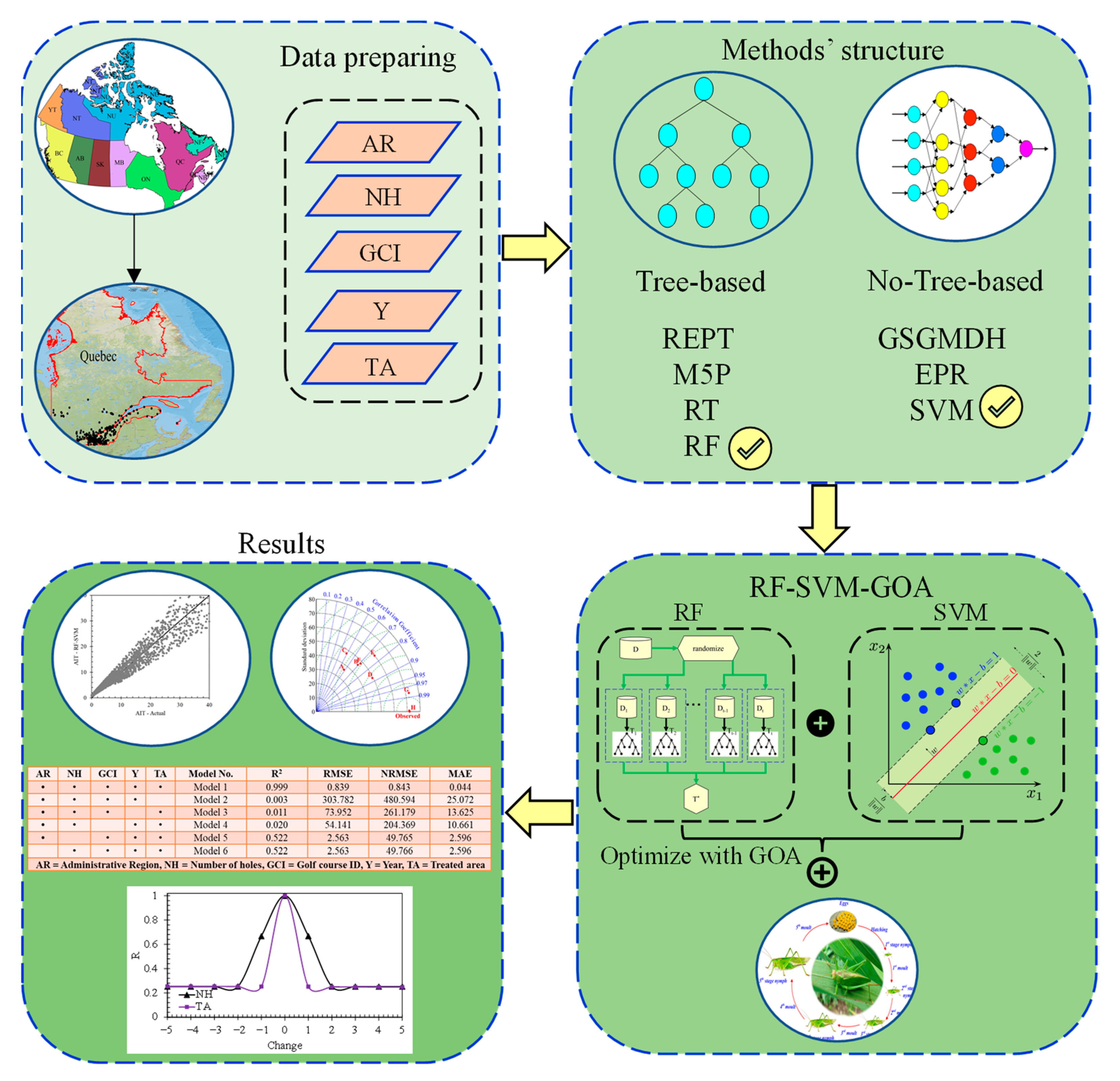
2. Materials and Methods

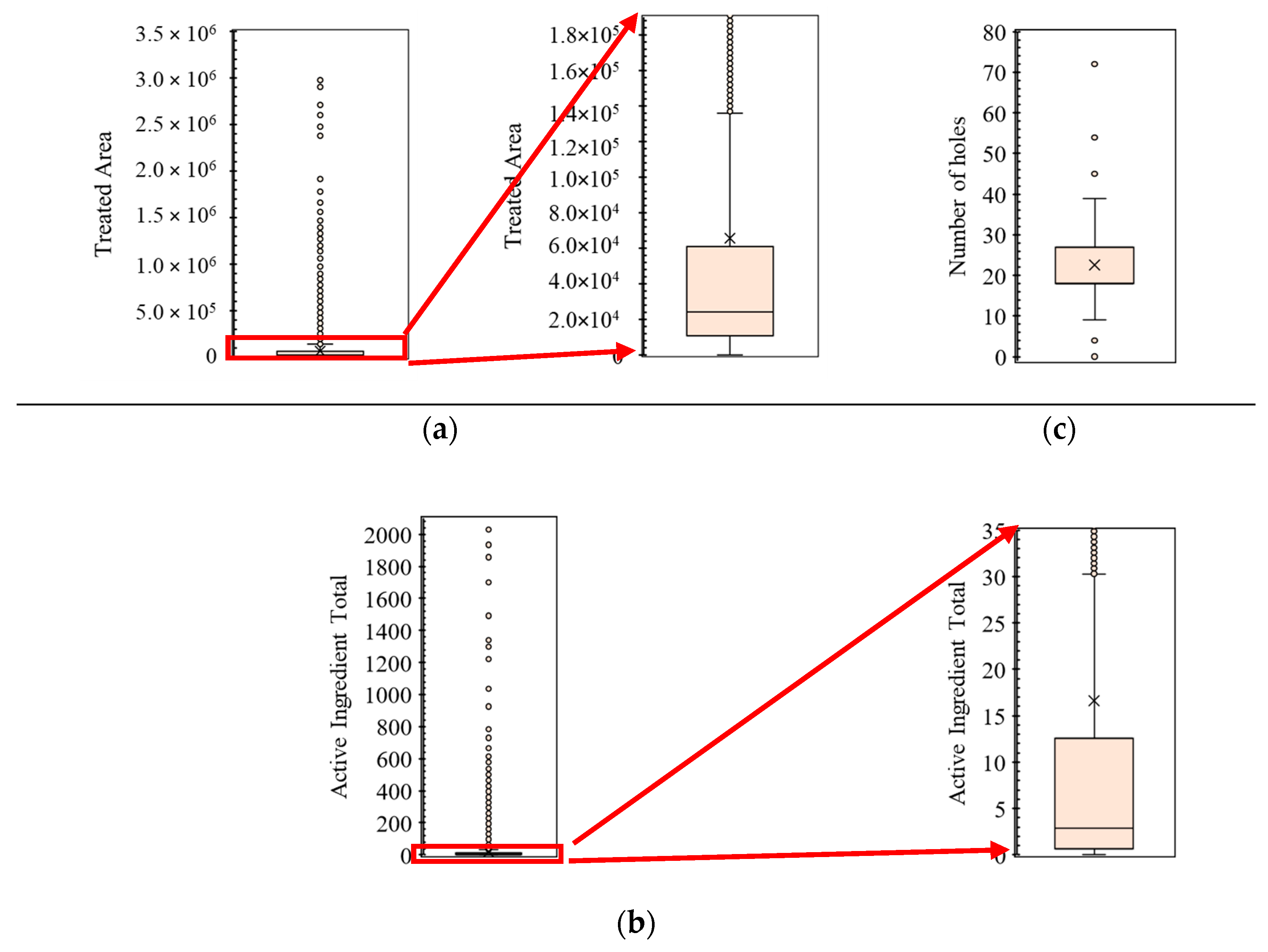
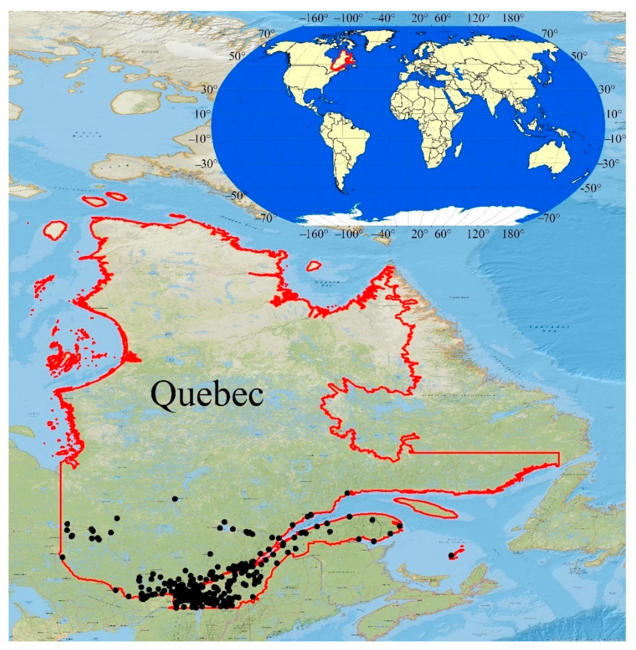
2.1. Golf Course Database

In the province of Québec, Canada, golf-course managers have been required by law, since 2003, to submit a pesticide reduction management plan every three years to the Ministère de l’Environnement et de la Lutte aux Changements Climatiques (MELCC, i.e., Québec Ministry of Environment). According to the provincial law [4], these plans must contain: (i) golf-course identification (name, address, and ownership); (ii) total golf-course surface (ha), including greens, fairways, tee boxes, sand traps, and rough; (iii) quantities of pesticides applied in the previous three years, including product name, registration number, and area treated; (iv) methods used to prevent pesticide migration outside the course; (v) methods used to monitor pests and to control them without the use of pesticide; (vi) pesticide reduction objectives for the next three years. These plans must be signed by a certified agronomist licensed by the Ordre des Agronomes du Québec (professional board of agronomists).

This regulation has allowed MELCC to compile a database of all the pesticides used on 380 golf courses in the province between 2003 and 2017. The geographical locations of the golf courses are indicated in Figure 1. Most of studied golf courses are located in the south of Québec, with some scattered in the east and west of the province.

The compilation of all the pesticide reduction plans received by the MELCC has resulted in a database of 13,220 unique pesticide applications. We used this database for the development of the ML model, using five input variables (treated area (TA), administrative region (AR), golf course ID (GFI), number of holes (NH), and year (Y)) and one output variable (AIT). We attributed to each golf course with its fixed number of holes a given ID number in the MDDELCC database (golf course ID). The treated area (square meters) corresponds to the area treated with a given pesticide, whereas the region corresponds to the administrative region (numbered 1 to 17) of the province of Québec where the golf course was located. For each application, we calculated AIT as AIT = Q × C, where Q is the quantity of pesticide applied in kilograms or liters and C is the concentration of the active ingredient in the applied pesticide in percentage. For modeling purposes, we randomly selected 70% of the 13,220 samples as calibration samples and the rest were used as validation samples.

The statistical indices of the independent input and dependent output variables are presented as box plots in Figure 2. In this figure, only two input variables (treated area and number of holes) are shown. Region and golf-course ID are only labels and should be treated as qualitative, not quantitative, variables. The same applies for years. Thus, we do not show boxplots for these three data series. We applied these parameters in models to help the classification method (i.e., random forest). Notably, we considered samples where the AIR was >3 times the maximum label rate as outliers and removed them from the database. We observed that the difference between the minimum and maximum TA and AIT were so large that, by reducing the range of numbers in Figure 2a,b, many of these samples were near to the minimum values of the variables.

Given the many samples in the high ranges of these variables, they could not be considered as outliers. Owing to this large variation in AIT as the outcome, the machine learning models faced considerable challenges in adjusting the model hyperparameters and in training to produce a model with a good prediction performance for all range of samples. The results of the ANOVA and Duncan’s multiple range tests [18] indicated a significant difference between the highest and lowest means of the input variables.

2.2. Theoretical Overview

In the current study, we developed a hybrid model by coupling a support vector machine (SVM) with random forest (RF) and the grasshopper optimization algorithm (GOA). The details of RF, SVM, and GOA are provided in Section 2.2.1, Section 2.2.2, and Section 2.2.3, respectively. The full details of the developed hybrid model are provided in Section 2.2.4.

2.2.1. Random Forest

RF is a powerful ensemble classifier that is robust against overfitting [19]. RF employs a set of classification and regression tree (CART) methodologies to map the independent input variables to the dependent output variable(s). The trees in RF are generated with a bagging approach through the selection of a subset of training samples with replacement. Some samples may be chosen multiple times, whereas some may not be chosen at all.

After we selected the training samples from all samples, generally, two-thirds (or four-fifths, or three-fourths) are applied as in-bag (IB) samples to train the trees. Using the rest of the samples (i.e., one-third, one-fifth, or one-fourth, respectively) known as out-of-bag (OOB) samples, internal cross-validation is performed to check the generalizability of the RF model for estimating unseen samples (i.e., OOB samples) [19].

Nodes are split by the random selection of the number of features (Mtry), which is a user-defined parameter; the decision trees (DTs) are individually generated without any pruning. By expanding the forest to the number of trees (Ntree) as another user-defined parameter, the RF produces a tree with low bias and high variance [19]. Using the arithmetic mean to average the probabilities of the produced classes by all generated trees, the final classification RF-based model is built. After generating an RF-based model, we assessed a new unlabeled sample against all DTs products in the ensemble RF model, and each tree votes for the class membership (CM). The CM with the maximum number of votes is selected as the final class.

2.2.2. Support Vector Machine (SVM)

SVM is a well-known robust, reliable, and efficient supervised machine learning technique applied to classification [20] and regression [21] problems. The modeling framework in this method is defined based on statistical learning [22]. Maximizing the hyperplane margin in SVM leads to maximizing the separation between classes. The training points closest to the maximum hyperplane margin are called support vectors, which are used to define the margin between classes.

Vapnik [22] defined the ε-insensitive loss function used to extend SVM for regression-based problems [23], which is known as support-vector regression. This method employs the theory of structural risk minimization to enhance model generalization, even if created with limited calibration samples. The main objective of the minimization process through the modeling phase is to find a function for the nonlinear mapping of multi-input data pairs to the output variables with a maximum error within a certain value range (i.e., ε) from the actual samples applied in the calibration phase.

Consider training data points as $\left\{\left(x_1,y_1\right),\dots ,\left(x_l,y_l\right)|x_i\in R^n,y_j\in R,\left(i,j=1,2,\dots ,l\right)\right\}$, where l is the number of training samples. To find an SVM-based function to estimate the dependent output variable, the nonlinear mapping is defined as:

$$g\left(h\right)=〈m\cdot \varphi \left(h\right)〉+d$$

(1)

where g(h) is the corresponding output variable of $h=\left(h_1,h_2,\dots ,h_n\right)$ as input variable(s); $m\in R^n$ denotes the weights vector, which approximates the location of a hyperplane; n is the number of input variables; $\varphi \left(h\right)$ is an irregular SVM-based function used to allocate input variables(s) to high-dimensional space; and $d\in R$ is the bias term, which specifies hyperplane offset from the source.

The ε-insensitive loss function applied by Vapnik [22] is defined as:

$${\left|y-g\left(h\right)\right|}_{\epsilon }=\max \left\{0,\left|y-g\left(h\right)-\epsilon \right|\right\},\epsilon >0.$$

(2)

An irregular SVM-based function that estimates all training samples with an error lower than ε enforces a hard constraint on the estimation error. Moreover, in practice, finding a function that can estimate all training samples with an error less than the specified value (i.e., ε) may not be possible. To accomplish this and allow errors above ε, two slack variables, ${\xi }_i^{*}$ and ξ_i, are defined, and the SVM optimization function is written as [20]:

$$\begin{array}{l}\mathrm{Minimize}:R_{SVM}=\frac{1}{2}‖m^2‖+C{\displaystyle \sum _{i=1}^l\left({\xi }_i-{\xi }_i^{*}\right)}\\ \mathrm{Subjected}\mathrm{to}:\left\{\begin{array}{l}{y}_i-\left\{m\cdot \varphi \left(h_i\right)+d\right\}\le \epsilon +{\xi }_i\\ \left\{m\cdot \varphi \left(h_i\right)+d\right\}-y_i\le \epsilon +{\xi }_i^{*}\\ {\xi }_i,{\xi }_i^{*}\ge 0\end{array}\right.\end{array}$$

(3)

All parameters presented in the above relation are already defined except C, which is the regularization parameter, which is a positive constant parameter.

The optimization problem in Equation (3) is solved using Lagrange multipliers. The details of the solution can be found in Smola and Scholkopf [24]. The solution to Equation (3) is:

$$\begin{array}{c}\mathrm{Maximum}:R_{SVM}=-\frac{1}{2}{\displaystyle \sum _{i=1}^l{\displaystyle \sum _{j=1}^l\left(b_i-b_i^{*}\right)}}\left(b_i-b_i^{*}\right)G\left(h_i-h_j\right)\hfill \\ \hspace{1em}\hspace{1em}\hspace{1em}\hspace{1em}\hspace{1em}\hspace{1em}\hspace{1em}-\epsilon {\displaystyle \sum _{i=1}^l\left(b_i-b_i^{*}\right)}+{\displaystyle \sum _{i=1}^l{y}_i\left(b_i-b_i^{*}\right)}\hfill \\ \mathrm{Subjected}\mathrm{to}:\left\{\begin{array}{l}{\displaystyle \sum _{i=1}^l\left(b_i-b_i^{*}\right)}=0\\ b_i,\hspace{0.17em}{b}_i^{*}\in \left[0,C\right]\end{array}\right.\hfill \end{array}$$

(4)

where $G\left(h_i-h_j\right)=\phi \left(h_i\right)\cdot \phi \left(h_j\right)$ denotes the kernel function. By solving the above equation, b_i and $b_i^{*}$ are obtained. Consequently, Equation (1) is rewritten as:

$$g\left(h\right)={\displaystyle \sum _{i=1}^l\left(b_i-b_i^{*}\right)}\hspace{0.17em}\hspace{0.17em}G\left(h_i,h_j\right)+d.$$

(5)

Using the kernel function in the optimization problem in Equation (4) instead of φ(h) substantially reduces the computational cost of solving high-dimensional feature space problems. Given the adaptability of the radial basis function (RBF) kernel function in handling complex parameters; the ease of adoption for adaptive and optimization techniques; and its reliability, simplicity, and computational efficiency [25], we applied it in our study. The mathematical formulation of the RBF kernel function is:

$$G\left(h_i,h_j\right)=\exp \left(-\gamma {‖h_i-h_j‖}^2\right)$$

(6)

where γ (γ = 1/2σ²) is the RBF parameter.

2.2.3. Grasshopper Optimization Algorithm (GOA)

GOA [26] imitates the social interactions and behavior of a grasshopper searching for food in nature to define a mathematical model in solving optimization problems. The grasshopper’s life cycle includes egg, nymph, and adult stages. The swarming behavior of grasshoppers occurs at both the nymph and adult stages [27]. Abruptly and locally moving as exploration and exploitation search processes as well as target seeking are naturally performed by grasshoppers.

The mathematical simulation of the swarming behavior of grasshoppers is defined with three main variables so that the position of the ith grasshopper (X_i) is defined as a function of wind advection (A_i), gravity force (G_i), and social interaction (S_i) as follows [28]:

$$X_i=A_i+G_i+S_i.$$

(7)

To describe the random behavior of grasshoppers, the above equation is rewritten as:

$$X_i=r_1{A}_i+r_2{G}_i+r_3{S}_i$$

(8)

where r₁, r₂, and r₃ are considered random through [0, 1].

The mathematical definitions of the three terms for estimating grasshopper position are:

$$A_i=u{\stackrel{⌢}{e}}_w$$

(9)

$$G_i=-g{\stackrel{⌢}{e}}_g$$

(10)

$$S_i={\displaystyle \sum _{\begin{array}{l}j=1\\ j\ne i\end{array}}^{N_g}s\left(d_{ij}\right){\stackrel{⌢}{d}}_{ij}}$$

(11)

where u and g are the drift and gravitational constants, respectively; ${\stackrel{⌢}{e}}_w$ and ${\stackrel{⌢}{e}}_g$ are unity vectors in the wind direction and toward the Earth’s center, respectively; s defines the power of social forces; d_ij (= x_j − x_i) is the distance between two grasshoppers; and ${\stackrel{⌢}{d}}_{ij}$ is a unit vector. The values ${\stackrel{⌢}{d}}_{ij}$ and s are defined as:

$$s(r)=f{e}^{\frac{-r}{l_s}}-e^{-r}$$

(12)

$${\stackrel{⌢}{d}}_{ij}=\frac{x_j-x_i}{d_{ij}}$$

(13)

where f is the attraction intensity and l_s is the attractive length scale.

Using a defined function for A, G, and S, the position of the ith grasshopper Equation (7) is rewritten as:

$$X_i={\displaystyle \sum _{\begin{array}{l}j=1\\ j\ne i\end{array}}^{N_g}s\left(\left|x_j-x_i\right|\right)\frac{x_j-x_i}{d_{ij}}}-g{\stackrel{⌢}{e}}_g+u{\stackrel{⌢}{e}}_w.$$

(14)

The above equation is modified to prevent the grasshoppers from early convergence [25].

$$X_i^d=c\left({\displaystyle \sum _{\begin{array}{l}j=1\\ j\ne i\end{array}}^{N_g}c\frac{u{b}_d-l{b}_d}{2}s\left(\left|x_j^d-x_i^d\right|\right)\frac{x_j-x_i}{d_{ij}}}\right)+{\stackrel{⌢}{T}}_d$$

(15)

where ub_d and lb_d are the upper and lower bounds in the dth dimension, respectively; s is a parameter defining the power of social forces Equation (11); ${\stackrel{⌢}{T}}_d$ is the value of the dth dimension (i.e., the best solution obtained so far); and c is a parameter used to shrink the attraction, repulsion, and comfort zones.

Among the parameters presented in Equation (7), S is very similar to the first term of Equation (13). We also assumed that the wind direction is always toward the target (${\stackrel{⌢}{T}}_d$), parameter A was omitted, and gravity (i.e., G) was ignored.

For balancing exploitation and exploration in GOA, parameter c must be reduced compared to the iteration number. The comfort zone is decreased by c in proportion to the iteration number. Using this process prevents the reduction in exploitation by enhancing the iteration number. It is defined as:

$$c=c_{\max }-k_l\frac{c_{\max }-c_{\min }}{K}$$

(16)

where c_min and c_max are the minimum and maximum values that Saremi et al. [26] recommended as 0.00001 and 1, respectively; k_l and K denote the current iteration and the maximum number of iterations, respectively.

To define the next position of the grasshoppers with the developed GOA-based equation Equation (14), the position of the target and all other grasshoppers as well as its current position must be considered. The first term of Equation (14) considers the position of the current grasshoppers in relation to the other ones. The position of the search agent in GOA is updated based on the positions of all other search agents, its current position, and the global best.

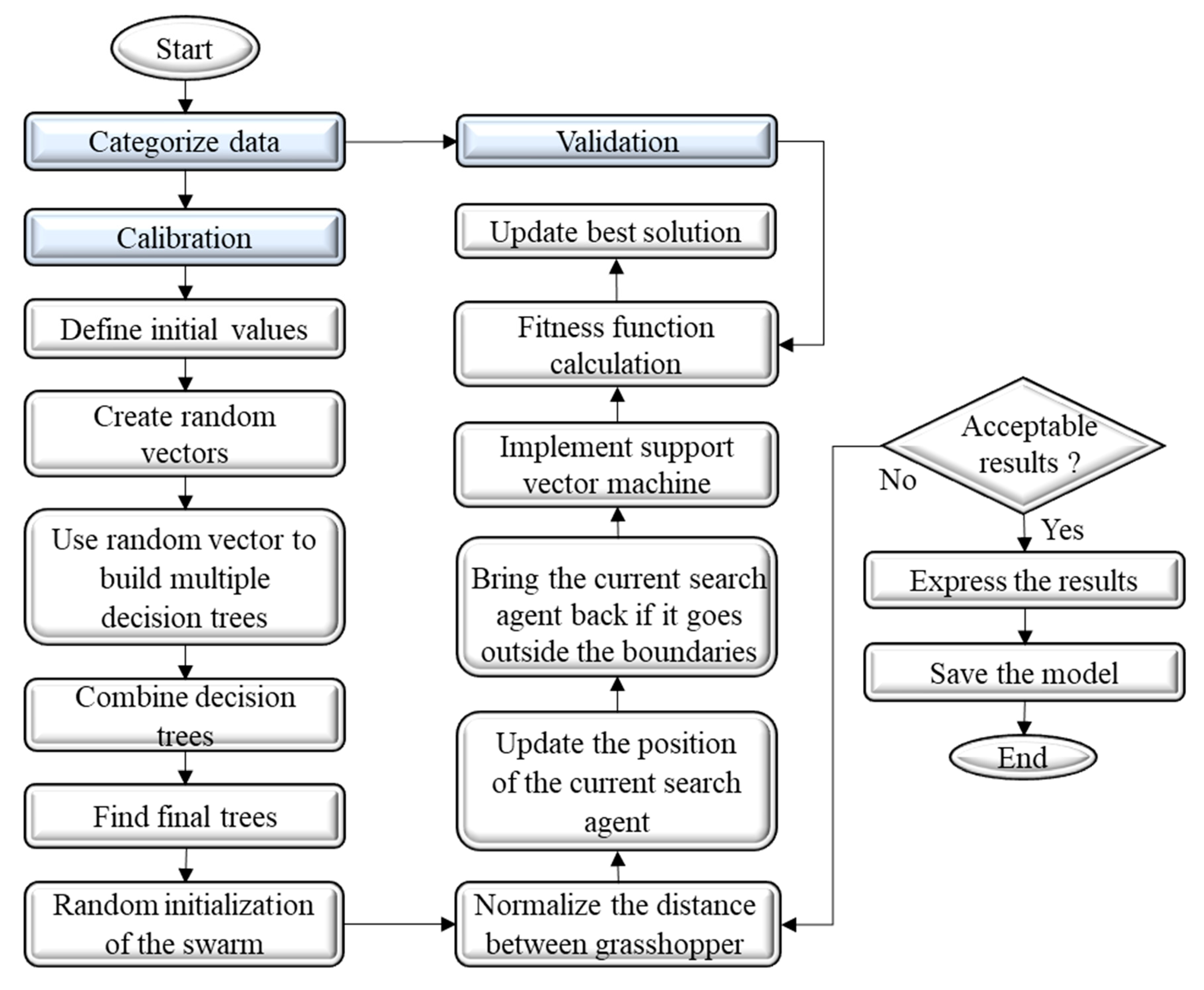
2.2.4. Developed Hybrid RF-SVM-GOA

The developed hybrid method is a new coupling of SVM with two different methods: RF as a classifier to handle the high range of samples and GOA as an optimization algorithm to find the optimal value of the SVM. The modeling of the developed RF-SVM-GOA model was performed by an integrated computer program in the MATLAB environment. Figure 3 depicts the flowchart of the developed hybrid techniques for AIT forecasting. The first step involves categorizing all samples into calibration and validation data. Using calibration samples, different random vectors are generated through the training phase based on the defined framework for RF and are employed to build multiple DTs. The created DTs are combined to produce the final trees. For each selected tree, random values for a predefined swarm are initialized, and the fitness function is calculated for this swarm. For the number of iterations defined by the user, the following step is performed: from the first iteration until reaching the maximum number of iterations, the reducing parameter used to shrink attraction and comfort zones, as well as repulsion (c), is updated by Equation (15). For all search agents, the distances between grasshoppers are normalized, the position of the current search agent is updated by Equation (14), and the boundaries of the current search agents are controlled. Next, the SVM is implemented, and the cost function is recalculated to find the best search agent. This process is repeated to reach all search agents at different iteration numbers as well as for all trees to find the final model for AIT forecasting.

Owing to the considerable differences between the minimum and maximum of the independent input variables as well as the dependent output variable, a hybrid model is required for AIT forecasting. In the current study, we considered two machine learning categories, including tree- and non-tree-based techniques, to find the optimal model for AIT forecasting. The tree-based techniques included M5P [29], random tree [30], REP tree [31], RF [32]; the non-tree-based techniques included GSGMDH [33], EPR [34], and SVM [35].

The main modeling challenge with ML techniques is adjusting the predefined hyperparameters of the model. The trial-and-error process is one of the well-known methods used for finding them; however, the process requires many trials to reach the optimal value of these hyperparameters for a given problem. Notably, the user experience also strongly impacts the faster identification of optimal values. In addition, the interaction of these parameters is a source of prediction errors; in such cases, the trial-and-error process faces considerable problems. Therefore, in order to find the values of the parameters of this method, evolutionary algorithms are used so that the values are found automatically and are used in modeling. Through a trial-and-error process, the optimized values of different parameters of the mentioned models were found and provided in

Table 1. Optimized values of parameters of different models.

Method	Parameter	Setting
RF	Bag size percentage	100
	Batch size	100
	Maximum depth of tree	10, 5
	Number of decimal places	2
	Number of execution slots	1
	Number of features	1
	Number of iterations	100
	Seeds	300, 10
RT	Number of randomly chosen attributes	0
	Minimum total weights of instances in a leaf	1
	Minimum proportion of the variance of all data that need to be present at a node for splitting to be performed in regression trees	0.001
	Seed	100
	Maximum depth of tree	5
REP Tree	Minimum total weights of instances in a leaf	2
	Minimum proportion of the variance of all data that need to be present at a node for splitting to be performed in regression trees	0.001
	Seed	100
	Maximum tree depth	5
M5P	Minimum number of instances to allow at a leaf node	20
	Number of decimal places to be used for output of numbers in model	20
GSGMDH	Maximum number of inputs for individual neurons	3
	Maximal number of neurons in a layer	10
	Degree of polynomials in neurons	3
EPR	Number of terms	50, 200
	Maximum number of iterations	50
	Population size	50
	Crossover percentage	0.35
	Mutation percentage	0.04
GOA	Maximum number of iterations	1000
	Number of search agents	70
	cmin	0.00001
	cmax	1

.

2.3. Performance Evaluation Criteria

According to the stochastic nature of AIT, considering only one criterion to assess the performance of each model would be insufficient. Therefore, we applied a group of statistical indices, including the correlation coefficient (R), mean absolute error (MAE), root mean square error (RMSE), and normalized RMSE (NRMSE), to evaluate the performance of the developed model for AIT forecasting. Simultaneously considering the mentioned indices is sufficient for evaluating the efficiency of a model [36]. The mathematical definitions of R, MAE, RMSE, and NRMSE are as follows, respectively:

$$R=\frac{l\left({\displaystyle \sum _{i=1}^l{A}_i{P}_i}\right)-\left({\displaystyle \sum _{i=1}^l{P}_i}\right)\left({\displaystyle \sum _{i=1}^l{A}_i}\right)}{\sqrt{\left(l\left({\displaystyle \sum _{i=1}^l{A}_i^2}\right)-{\left({\displaystyle \sum _{i=1}^l{A}_i}\right)}^2\right)\left(l\left({\displaystyle \sum _{i=1}^l{P}_i^2}\right)-{\left({\displaystyle \sum _{i=1}^l{P}_i}\right)}^2\right)}}$$

(17)

$$MAE=\frac{{\displaystyle \sum _{i=1}^l\left|P_i-A_i\right|}}{l}$$

(18)

$$RMSE=\sqrt{\frac{{\displaystyle \sum _{i=1}^l{\left(P_i-A_i\right)}^2}}{l}}$$

(19)

$$NRMSE=\frac{1}{{\displaystyle \sum _{i=1}^l{A}_i}}\sqrt{\frac{{\displaystyle \sum _{i=1}^l{\left(P_i-A_i\right)}^2}}{l}}$$

(20)

where l is the number of samples; P_i and A_i are the predicted and actual (respectively) ith sample values, respectively.

3. Results and Discussion

Figure 4 graphically represents the AIT modeling in the current study. As shown in the figure, the modeling involves four main steps: (1) data preparation, (2) methods’ structure, (3) developing hybrid model, and (4) results. The details of data preparation are presented in Section 2.1, and the details of the methods’ structure and the development of the hybrid model are provided in Section 2.2. Finally, our results are provided in this section. The first step of the results involved comparing the tree- and non-tree-based individual models. After the comprehensive comparison, we selected and compared the best tree- and non-tree-based models. We also applied the GOA to optimize the model’s variables. We compared all individual models and the developed hybrid model using a Taylor diagram. After confirming the superiority of the developed method, we checked each input variable’s effect in estimating the target parameter. Finally, we evaluated the impact of changes in input variables on the results of the developed model.

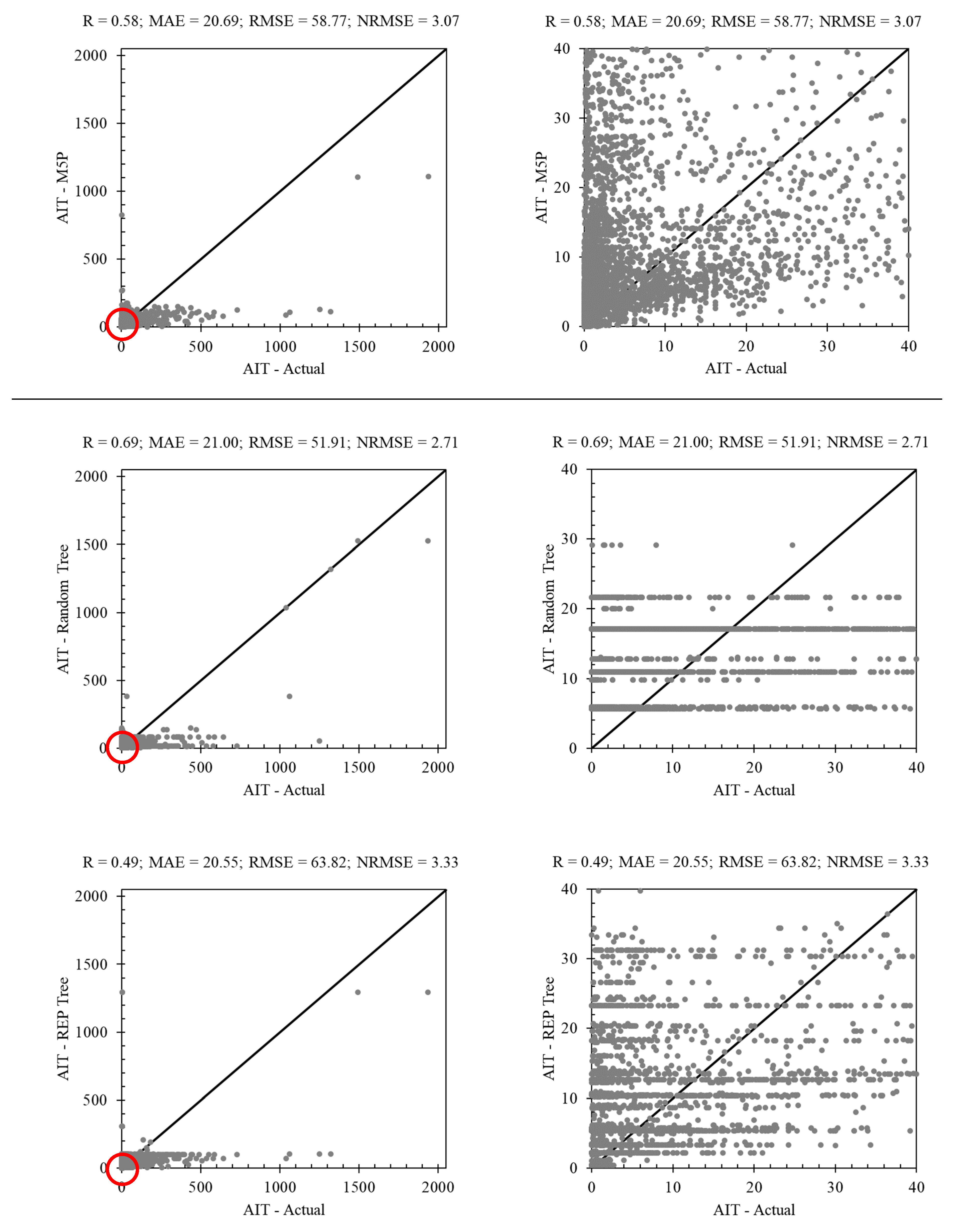
3.1. Tree-Based Methods in AIT Estimating

Figure 5 indicates the AIT forecasting results of four tree-based techniques: M5P, random tree, REP tree, and RF. The results of this figure show that M5P was not able to accurately predict high AIT values, with an R of 0.58, which indicated the poor performance of the model for high values of the target variable. In addition, this method performed poorly for low AIT values, both over- and underestimating the high relative error for some samples. The correlation coefficient of the random tree (R = 0.69) was higher than that of the M5P. This model still produced some large relative errors for high and low AIT. The random tree method did not perform well for low AIT, so most values in the range of 0 < AIT < 40 were estimated with high error. A comparison of the M5P and random tree results in terms of statistical indices demonstrated that random tree (R = 0.69; MAE = 21.00; RMSE = 51.91; NRMSE = 2.71) outperformed M5P (R = 0.58; MAE = 20.69; RMSE = 58.77; NRMSE = 3.07).

The third method proposed for estimating AIT is the REP tree. This method did not show an acceptable ability to estimate AIT. A quantitative comparison of the results of the REP tree (R = 0.49; MAE = 20.55; RMSE = 63.82; NRMSE = 3.33) with those of the other two methods showed that this method did not perform better than M5P or random tree (i.e., REP tree < M5P < random tree). The statistical indices of these methods were close. The last tree-based method is the RF method. According to the initial modeling performed by this method, we observed that the use of a relatively simple model based on RF can substantially increase the modeling performance compared with other methods (i.e., random tree, M5P, and REP tree). To increase the modeling accuracy to achieve the optimum results, we performed AIT modeling with another complex RF-based technique. The increased complexity is acceptable as long as overfitting does not occur. The performance of the model for unseen samples also must be acceptable. Therefore, the proposed models based on this method were complex (C) and simple (S). A comparison of RF (S) (R = 0.70; MAE = 19.60; RMSE = 51.86; NRMSE = 2.71) with other tree-based methods showed that the quantitative performance of this model was better than those of other tree-based models. Although this method did not perform well for low AIT, the result produced by RF was more acceptable than produced by the best of the other methods (i.e., random tree). In addition, the use of complex RF (C) (R = 0.87; MAE = 15.85; RMSE = 37.37; NRMSE = 1.95) considerably increased the values of the numerical indices compared with the other methods. However, to ensure the acceptable performance of this method, its performance in a different range of AIT should also be examined. Although the complex RF-based model performed better than the other methods as well as simple RF, this method did not perform well in the range of 0 < AIT < 500. Therefore, non-tree-based methods or hybrid methods should be considered to construct an optimal method for AIT modeling.

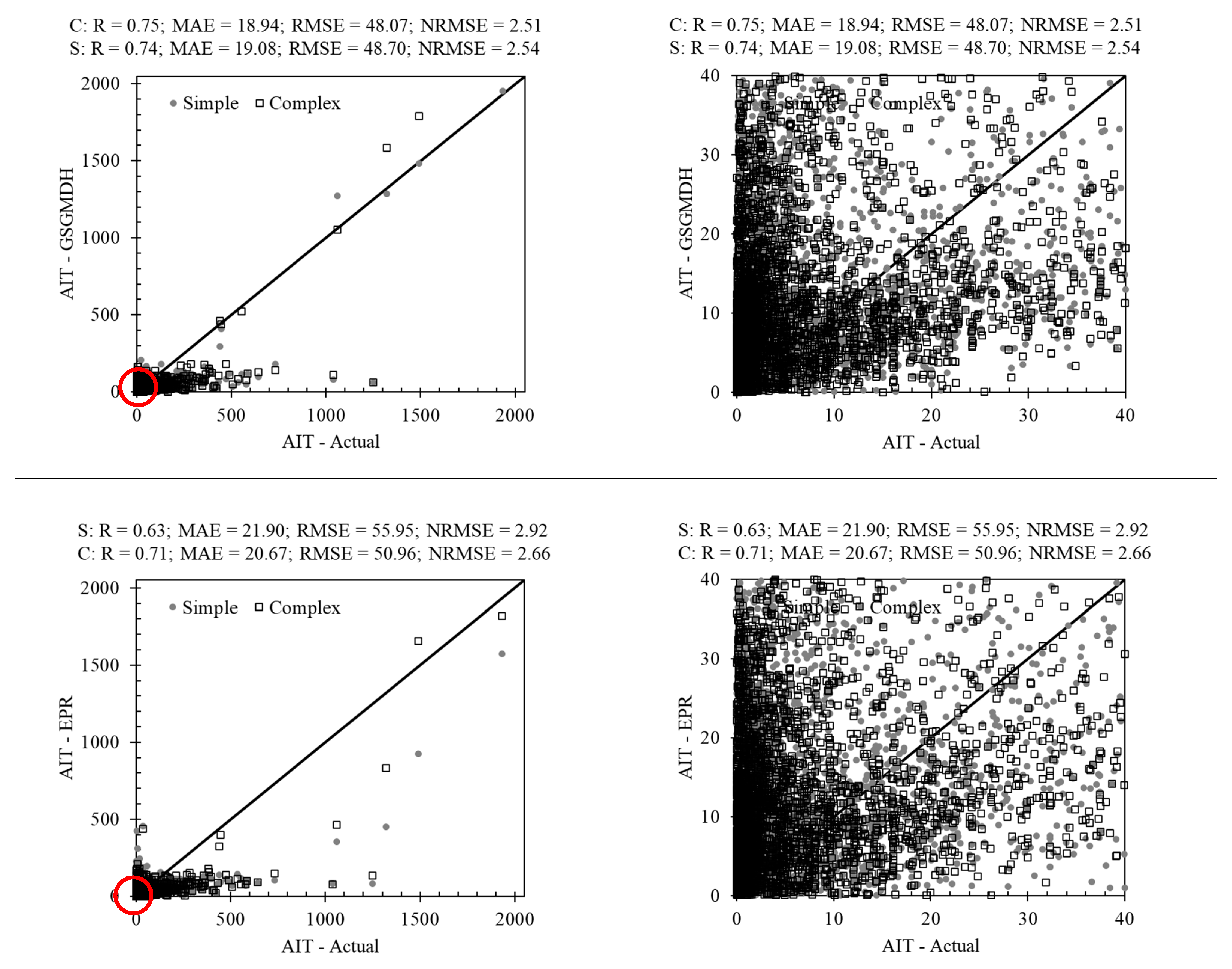
3.2. Non-Tree-Based Methods in AIT Estimating

Figure 6 shows the scatter plot of the results of the two non-tree-based techniques in AIT forecasting. The applied methods were evolutionary polynomial regressions (EPR) and generalized structure of group method of data handling (GSGMDH). We used these two methods because of the successful performance of these newly developed methods in solving recent complex real-world problems. Increasing the complexity of these two methods may lead to stronger models in predicting the target parameter. In this study, we considered two models, simple and complex, as with RF, for both methods. The increasing complexity of this model did not lead to overfitting. The notable result regarding these methods is that both, despite the reports of good performance in solving nonlinear problems, produced poor results for all AIT ranges. Therefore, the next option to find an efficient model in AIT estimation was using a hybrid model.

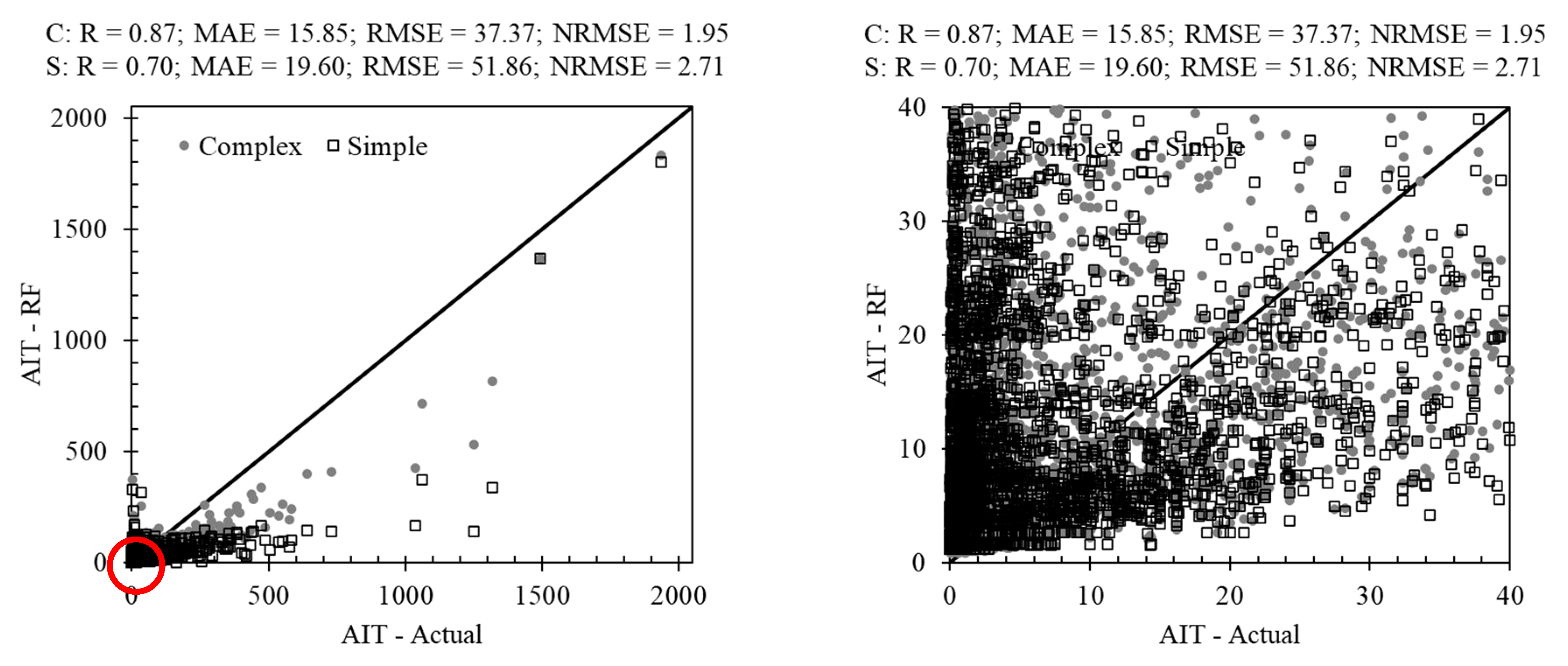
3.3. AIT Estimating Using Hybrid Methods

Figure 7 demonstrates the scatter plot of the hybrid techniques in AIT forecasting. The developed hybrid models included SVM integrated with RF (RF-SVM) and SVM integrated with RF and GOA. Both developed hybrid models performed well in AIT forecasting: the statistical indices of RF-SVM (R = 0.98; MAE = 3.32; RMSE = 13.3; NRMSE = 0.69) and RF-SVM-GOA (R = 0.99; MAE = 0.84; RMSE = 0.84; NRMSE = 0.04) are better than those of the considered tree- and non-tree-based techniques. A comparison of RF-SVM and RF-SVM-GOA for an AIT of less than 40 indicated the poor performance of RF-SVM: most samples were underestimated or overestimated with high relative error. However, RF-SVM-GOA performed well in this range. This model overestimated in the range of [0, 8] and both overestimated and underestimated in the range of [8, 40] but the relative error of RF-SVM-GOA was much lower than that of RF-SVM. A comparison of these two methods showed the importance of coupling SVM with GOA to find the optimum values of SVM for all defined categories in the RF.

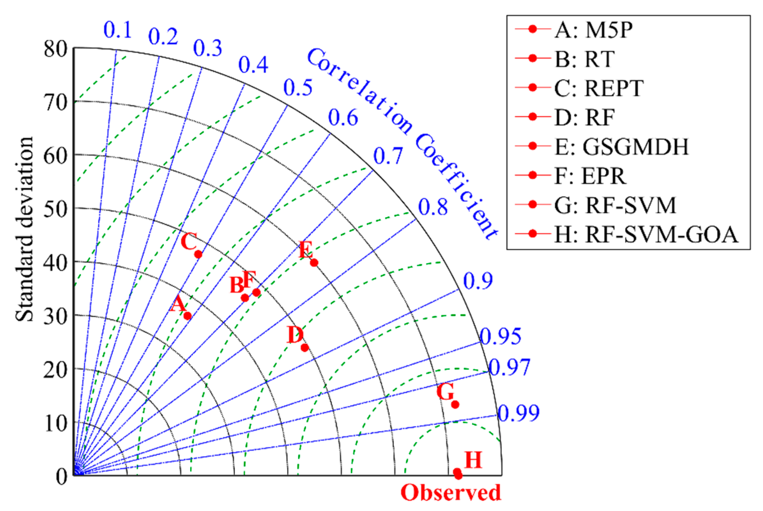
3.4. Comparison of the Individual and Hybrid Methods in AIT Estimating

Figure 8 plots a Taylor graph for the comparison of the different developed techniques (individual methods including tree- and non-tree based and hybrid models) in AIT forecasting. A Taylor graph [37] is a graph that simultaneously compares different models by using three indices: correlation coefficient, standard deviation, and RMSE. The model with the shortest distance from the observed point has the best performance. Therefore, the models we developed ranked in descending order as RF-SVM-GOA, RF-SVM, RF, GSGMDH, EPR, RT, M5P, and REP tree (REPT).

3.5. Evaluation of the Importance of Each of the Input Parameters in AIT Estimating

The effect of each independent input variable on AIT forecasting using the developed hybrid technique is shown in

Table 2. Effect of each independent input variable on AIT forecasting using developed hybrid technique.

AR	NH	GCI	Y	TA	Model No.	R2	RMSE	NRMSE	MAE
•	•	•	•	•	1	0.999	0.839	0.843	0.044
•	•	•	•		2	0.003	303.782	480.594	25.072
•	•	•		•	3	0.011	73.952	261.179	13.625
•	•		•	•	4	0.020	54.141	204.369	10.661
•		•	•	•	5	0.522	2.563	49.765	2.596
	•	•	•	•	6	0.522	2.563	49.766	2.596

AR = administrative region, NH = number of holes, GCI = golf course ID, Y = year, TA = treated area.

. According to this table, removing the treated area (TA) from the model inputs (Model 2) substantially reduced the modeling accuracy compared with Model 1. Furthermore, the correlation coefficient of Model 2 was less than 1% of the value of this index for Model 1, whereas the RMSE, NRMSE, and MAE indices for Model 2 were more than 362, 570, and 570 (respectively) times higher than for Model 1. Removing Y and GCI as input variables also decreased the AIT modeling accuracy. Although Models 5 and 6 performed poorly in AIT estimation, their accuracy was higher than that of Model 2. Similar to the three variables GCI, TA, and Y, not using the two variables NH and R (Models 5 and 6) affected the modeling results. However, the importance of these two variables (i.e., NH and AR) was lower than that of the others. The correlation coefficients of Models 5 and 6 were 47% lower than that of Model 1. The values of RMSE, NRMSE and MAE for Models 5 and 6 were more than 3, 59, and 59 times higher than in Model 1. TA, Y, GCI, NH, and AR ranked first to fifth, respectively, in terms of the effect of the input variable.

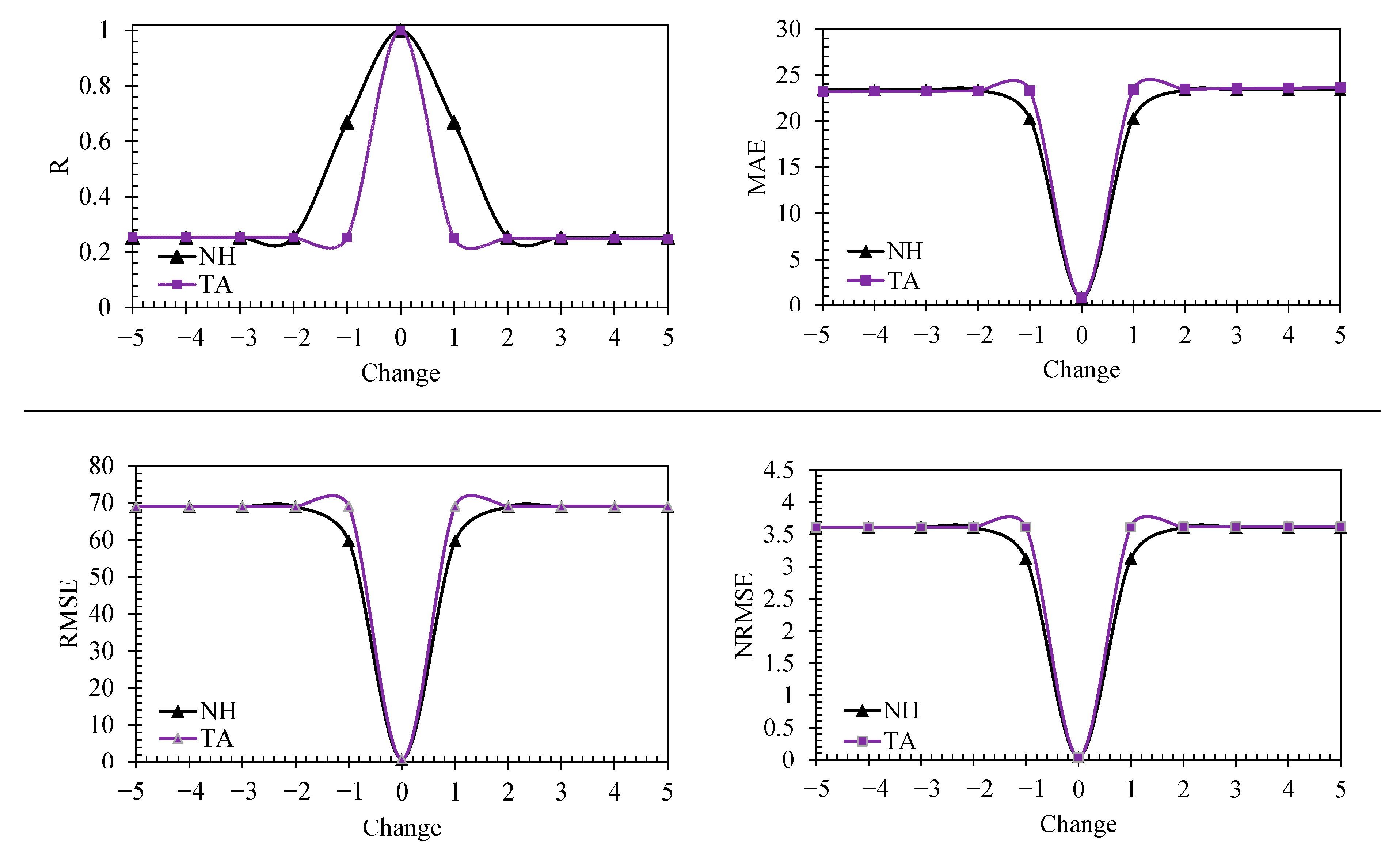
3.6. Sensitivity of the Developed Models on the Input Variables

Figure 9 shows the impact of the number of holes (NH) and treated area (TA) on the performance of the developed RF-SVM-GOA model. For the number of holes (NH) and treated area (TA), we considered changes of ±5 to ±10, and ±5% to ±10%. However, after ±5%, we observed almost no changes. A unit change in the NH resulted in more than a 33% reduction in R, whereas a 1% change in TA resulted in a more than 74% in R. A decrease of five units led to a substantial decrease in R: close to 0.3 for both. In addition, increasing the TA value by 5% reduced the correlation coefficient of the model to R = 0.25. Similar to the R, the largest decrease in modeling accuracy occurred in the first 1%. For example, the percentage changes in the different indices due to a 1% change in TA were R = 75%, MAE = 2683%, RMSE = 8092%, and NRMSE = 8092%. Therefore, we observed that the proposed model is sensitive to the values of different variables, which should be considered when measuring this variable and was expected given the wide ranges of input and output data.

4. Advantages, Limitations, and Future Improvements

The hybrid model that we developed was successful in estimating the actual ingredient total (AIT). The main advantage of the proposed method is not only accurate AIT forecasting but also the automatic finding of SVM variables and the automatic classification of the main calibration samples to overcome the limitation of machine learning in real-world problem modeling when the range of sample values is wide. Previous research using machine learning to predict pesticide behavior [38] or crop risks [39] relied mostly on either tree-based methods or artificial neural networks. However, a mixed approach, using a gradient boosting regression tree coupled to extended connectivity fingerprints, has been previously used to predict pesticide dissipation in plants [40].

In the current study, we applied GOA to find the optimal values of the SVM. The main advantage of GOA is updating the grasshopper’s position not only using the best solution found so far, but also the positions of all the other grasshoppers. This is an advantage of GOA over other nature-inspired optimization algorithms such as particle swarm optimization and genetic algorithm [26]. The other advantages of this optimization algorithm are its fast convergence even in unknown search spaces [26,41] and its continuous exploitation and exploration abilities [26]. However, the developed hybrid model can also be implemented by newly introduced nature-inspired machine learning methods such as the Salp swarm algorithm (SSA). To our knowledge, the current study is the first one to combine different types of machine learning from two different categories (i.e., REPTree, M5P, RT, and RF as tree-based methods and GSGMDH, EPR, and SVM as non-tree-based methods) for estimation of the pesticide use on golf courses.

The challenges that prevent improvement in applying and developing machine learning in AIT forecasting must be considered. The existing challenges related to analyzing and estimating AIT are as follows:

Modeling challenges: The main modeling challenges in the current study for a computer with an Intel Core i7 processor and 10 GB RAM included: (i) finding the optimum value of parameters for each ML model, (ii) needing to run the model with a large number of iterations (1000–100,000), (iii) the long training time required for most of the models (one hour to more than one day), (iv) the low memory available for running other powerful machine learning approaches such as individual support vector machine and adaptive neuro-fuzzy inference system (ANFIS) due to the complexity of the problem samples resulting in out-off memory, and (v) the more than 780,000 runs required to calculate the sensitivity.

Data challenges: The main challenge with the data was the number of large samples with small independent variables that we had for mapping the dependent output variable and input variables. The many samples resulted in a time-consuming modeling process, especially for the current study, where we coupled RF and GOA with SVM.

We developed this model using data that were available under the current regulations in the province of Québec. However, other factors affecting pesticide use on golf courses are not considered in these regulations. For example, Bekken et al. [2] showed a correlation between pesticide use and golf course economic data such as revenue per hectare and maintenance budget. Other factors, such as superintendent experience and level of education, golfers’ expectations, and local environment characteristics may also affect pesticide use but are not included in our proposed model.

5. Conclusions

In the current study, we developed a new hybrid supervised machine-learning-based model for pesticide application forecasting, expressed as actual ingredient total (AIT), on golf courses. This model can help Québec golf-course managers more accurately predict their pesticide use and be more efficient in setting their pesticide-reduction objectives as required by the current regulations. Agronomists and regulatory authorities can also use the model to better refine the process through which golf courses set and achieve their objectives in pesticide reduction. For example, favorable economic measures can be implemented for golf courses that use less pesticides than the amount predicted by the model. Furthermore, this model can be adapted to other crops where reductions in pesticide use are required if a database of pesticide applications is available.

This hybrid technique is a new coupling of the support vector machine (SVM) method with random forest (RF) and grasshopper optimization algorithm (GOA). To estimate AIT, we considered five independent input variables: year (Y), golf course ID (GCI), administrative region (AR), treated area (TA), and number of holes (NH). We compared the results of the developed RF-SVM-GOA with those of four tree-based techniques including M5P, random tree, reduced error pruning tree (REP tree), and RF, and those of non-tree-based techniques including the generalized structure of group method of data handling (GSGMDH) and evolutionary polynomial regression (EPR). The comparison of the results indicated that RF-SVM-GOA (R = 0.99; MAE = 0.86; RMSE = 0.87; NRMSE = 0.04) outperformed the tree- and non-tree-based techniques. The supervised machine learning methods we developed in the current study ranked in descending order as RF-SVM-GOA, RF-SVM, RF, GSGMDH, REP tree (REPT), RT, M5P, and EPR. By removing one of the input variables for each model, we defined six different models to find the optimal input combination. The results of the defined models showed that AR and NH had the least impact on AIT forecasting, whereas TA was the most effective input variable. Using the optimum model with five input variables, we performed a sensitivity analysis to determine the sensitivity of the developed model to each input variable. The results demonstrated the high sensitivity of the developed RF-SVM-GOA method compared to those of the other considered methods; the highest sensitivity was related to TA and the sensitivities to NH and Y were similar. In a future step, climatic variables such as precipitation and temperature will be used as input variables to improve the developed hybrid model for forecasting AIT in the future based on the different climate change scenarios.

References

1. Stier, J.C.; Steinke, K.; Ervin, E.H.; Higginson, F.R.; McMaugh, P.E. Turfgrass Benefits and Issues. In Turfgrass: Biology, Use, and Management, 1st ed.; Stier, J.C., Horgan, B.P., Bonos, S.A., Eds.; Wiley: Hoboken, NJ, USA, 2013; Volume 56, pp. 105–145. [Google Scholar]
2. Bekken, M.A.; Schimenti, C.S.; Soldat, D.J.; Rossi, F.S. A novel framework for estimating and analyzing pesticide risk on golf courses. Sci. Total Environ. 2021, 783, 146840. [Google Scholar] [CrossRef]
3. Millington, B.; Wilson, B. An unexceptional exception: Golf, pesticides, and environmental regulation in Canada. Int. Rev. Sociol. Sport 2016, 51, 446–467. [Google Scholar] [CrossRef]
4. Metcalfe, T.L.; Dillon, P.J.; Metcalfe, C.D. Detecting the transport of toxic pesticides from golf courses into watersheds in the Precambrian Shield region of Ontario, Canada. Environ. Toxicol. Chem. 2008, 27, 811–818. [Google Scholar] [CrossRef]
5. Knopper, L.D.; Lean, D.R. Carcinogenic and genotoxic potential of turf pesticides commonly used on golf courses. J. Toxicol. Environ. Health Part B 2004, 7, 267–279. [Google Scholar] [CrossRef]
6. Gouvernement du Québec. Ministère de l’Environnement et de la Lutte aux Changements ClimatiquesI; Loi sur les Pesticides, L.R.Q., Chapitre P-9.3; Gouvernement du Québec: Quebec City, QC, Canada, 2022.
7. Baris, R.D.; Cohen, S.Z.; Barnes, N.L.; Lam, J.; Ma, Q. Quantitative analysis of over 20 years of golf course monitoring studies. Environ. Toxicol. Chem. 2010, 29, 1224–1236. [Google Scholar]
8. Abadi, B. The determinants of cucumber farmers’ pesticide use behavior in central Iran: Implications for the pesticide use management. J. Clean. Prod. 2018, 205, 1069–1081. [Google Scholar] [CrossRef]
9. Gan, H.; Wickings, K. Soil ecological responses to pest management in golf turf vary with management intensity, pesticide identity, and application program. Agric. Ecosyst. Environ. 2017, 246, 66–77. [Google Scholar] [CrossRef]
10. Mackey, M.J.; Connette, G.M.; Peterman, W.E.; Semlitsch, R.D. Do golf courses reduce the ecological value of headwater streams for salamanders in the southern Appalachian Mountains? Landsc. Urban Plan. 2014, 125, 17–27. [Google Scholar] [CrossRef]
11. Smith, M.D.; Conway, C.J.; Ellis, L.A. Burrowing owl nesting productivity: A comparison between artificial and natural burrows on and off golf courses. Wildl. Soc. Bull. 2005, 33, 454–462. [Google Scholar] [CrossRef]
12. Wong, H.; Haith, D.A. Volatilization of Pesticides from Golf Courses in the United States: Mass Fluxes and Inhalation Health Risks. J. Environ. Qual. 2003, 42, 1615–1622. [Google Scholar] [CrossRef]
13. Kearns, C.A.; Prior, L. Toxic greens: A preliminary study on pesticide usage on golf courses in Northern Ireland and potential risks to golfers and the environment. Saf. Secur. Eng. V 2013, 134, 173. [Google Scholar]
14. Yang, M.; Cho, S.I. High-Resolution 3D Crop Reconstruction and Automatic Analysis of Phenotyping Index Using Machine Learning. Agriculture 2021, 11, 1010. [Google Scholar] [CrossRef]
15. Diao, W.; Liu, G.; Zhang, H.; Hu, K.; Jin, X. Influences of Soil Bulk Density and Texture on Estimation of Surface Soil Moisture Using Spectral Feature Parameters and an Artificial Neural Network Algorithm. Agriculture 2021, 11, 710. [Google Scholar] [CrossRef]
16. Huang, L.; Wu, K.; Huang, W.; Dong, Y.; Ma, H.; Liu, Y.; Liu, L. Detection of Fusarium Head Blight in Wheat Ears Using Continuous Wavelet Analysis and PSO-SVM. Agriculture 2021, 11, 998. [Google Scholar] [CrossRef]
17. Carisse, O.; Fall, M.L. Decision Trees to Forecast Risks of Strawberry Powdery Mildew Caused by Podosphaera aphanis. Agriculture 2021, 11, 29. [Google Scholar] [CrossRef]
18. Oman, K.; Barwicki, J.; Rzodkiewicz, W.; Dawidowski, M. Evaluation of mechanical and energetic properties of the forest residues shredded chips during briquetting process. Energies 2021, 14, 3270. [Google Scholar]
19. Breiman, L. Random forests. Mach. Learn. 2001, 45, 5–32. [Google Scholar] [CrossRef] [Green Version]
20. Bonakdari, H.; Jamshidi, A.; Pelletier, J.P.; Abram, F.; Tardif, G.; Martel-Pelletier, J.A. Warning machine learning algorithm for early knee osteoarthritis structural progressor patient screening. Ther. Adv. Musculoskelet. Dis. 2021, 13, 1759720X21993254. [Google Scholar] [CrossRef] [PubMed]
21. Sharafi, H.; Ebtehaj, I.; Bonakdari, H.; Zaji, A.H. Design of a support vector machine with different kernel functions to predict scour depth around bridge piers. Nat. Hazards 2016, 84, 2145–2162. [Google Scholar] [CrossRef]
22. Vapnik, V.N. The Nature of Statistical Learning Theory, 1st ed.; Springer: Berlin, Germany, 2000. [Google Scholar]
23. Azimi, H.; Bonakdari, H.; Ebtehaj, I. Design of radial basis function-based support vector regression in predicting the discharge coefficient of a side weir in a trapezoidal channel. Appl. Water Sci. 2019, 9, 78. [Google Scholar] [CrossRef] [Green Version]
24. Smola, A.J.; Schölkopf, B. A tutorial on support vector regression. Stat. Comput. 2004, 14, 199–222. [Google Scholar] [CrossRef] [Green Version]
25. Ebtehaj, I.; Bonakdari, H. A support vector regression-firefly algorithm-based model for limiting velocity prediction in sewer pipes. Water Sci. Technol. 2016, 73, 2244–2250. [Google Scholar] [CrossRef] [PubMed] [Green Version]
26. Saremi, S.; Mirjalili, S.; Lewis, A. Grasshopper optimisation algorithm: Theory and application. Adv. Eng. Softw. 2017, 105, 30–47. [Google Scholar] [CrossRef] [Green Version]
27. Rogers, S.M.; Matheson, T.; Despland, E.; Dodgson, T.; Burrows, M.; Simpson, S.J. Mechanosensory-induced behavioural gregarization in the desert locust Schistocerca gregaria. J. Exp. Biol. 2003, 206, 3991–4002. [Google Scholar] [CrossRef] [PubMed] [Green Version]
28. Topaz, C.M.; Bernoff, A.J.; Logan, S.; Toolson, W. A model for rolling swarms of locusts. Eur. Phys. J. Spec. Top. 2008, 157, 93–109. [Google Scholar] [CrossRef] [Green Version]
29. Akhbari, A.; Zaji, A.H.; Azimi, H.; Vafaeifard, M. Predicting the discharge coefficient of triangular plan form weirs using radian basis function and M5’methods. J. Appl. Res. Water Wastewater 2017, 4, 281–289. [Google Scholar]
30. Kevric, J.; Jukic, S.; Subasi, A. An effective combining classifier approach using tree algorithms for network intrusion detection. Neural Comput. Appl. 2017, 28, 1051–1058. [Google Scholar] [CrossRef]
31. Ojha, V.K.; Schiano, S.; Wu, C.Y.; Snášel, V.; Abraham, A. Predictive modeling of die filling of the pharmaceutical granules using the flexible neural tree. Neural Comput. Appl. 2018, 29, 467–481. [Google Scholar] [CrossRef] [Green Version]
32. Zhu, H.J.; Jiang, T.H.; Ma, B.; You, Z.H.; Shi, W.L.; Cheng, L. HEMD: A highly efficient random forest-based malware detection framework for Android. Neural Comput. Appl. 2018, 30, 3353–3361. [Google Scholar] [CrossRef]
33. Safari, M.J.S.; Ebtehaj, I.; Bonakdari, H.; Es-haghi, M.S. Sediment transport modeling in rigid boundary open channels using generalize structure of group method of data handling. J. Hydrol. 2019, 577, 123951. [Google Scholar] [CrossRef]
34. Bonakdari, H.; Ebtehaj, I.; Akhbari, A. Multi-objective evolutionary polynomial regression-based prediction of energy consumption probing. Water Sci. Technol. 2017, 75, 2791–2799. [Google Scholar] [CrossRef] [PubMed]
35. Ebtehaj, I.; Bonakdari, H.; Shamshirband, S.; Mohammadi, K. A combined support vector machine-wavelet transform model for prediction of sediment transport in sewer. Flow Meas. Instrum. 2016, 47, 19–27. [Google Scholar] [CrossRef]
36. Legates, D.R.; McCabe, G.J., Jr. Evaluating the use of “goodness-of-fit” measures in hydrologic and hydroclimatic model validation. Water Resour. Res. 1999, 35, 233–241. [Google Scholar] [CrossRef]
37. Taylor, K.E. Summarizing multiple aspects of model performance in a single diagram. J. Geophys. Res. 2001, 106, 7183–7192. [Google Scholar] [CrossRef]
38. Qian, S.S.; Anderson, C.W. Exploring factors controlling the variability of pesticide concentrations in the Willamette River Basin using tree-based models. Environ. Sci. Technol. 1999, 33, 3332–3340. [Google Scholar] [CrossRef]
39. Yan, Y.; Feng, C.C.; Wan, M.P.H.; Chang, K.T.T. Multiple Regression and Artificial Neural Network for the Prediction of Crop Pest Risks. In Proceedings of the International Conference on Information Systems for Crisis Response and Management in Mediterranean Countries, Tunis, Tunisia, 28–30 October 2015; pp. 73–84. [Google Scholar]
40. Shen, Y.; Zhao, E.; Zhang, W.; Baccarelli, A.A.; Gao, F. Predicting pesticide dissipation half-life intervals in plants with machine learning models. J. Hazard. Mater. 2022, 436, 129177. [Google Scholar] [CrossRef]
41. Ibrahim, H.T.; Mazher, W.J.; Ucan, O.N.; Bayat, O. A grasshopper optimizer approach for feature selection and optimizing SVM parameters utilizing real biomedical data sets. Neural Comput. Appl. 2019, 31, 5965–5974. [Google Scholar] [CrossRef]
Figure 1. The geographical locations of the golf courses.
Agriculture 12 00933 g001
Figure 2. Box plots of the independent input and dependent output variables: (a) treated area (TA); (b) active ingredient total (AIT); (c) number of holes (NH).
Agriculture 12 00933 g002
Figure 3. The flowchart of the developed hybrid technique for AIT forecasting.
Agriculture 12 00933 g003
Figure 4. Graphical representation of the results.
Agriculture 12 00933 g004
Figure 5. Scatter plot of the tree-based techniques in AIT forecasting. Plots on the right are a scaled-up view of the region circled in red in the left plot.
Agriculture 12 00933 g005aAgriculture 12 00933 g005b
Figure 6. Scatter plot of the non-tree-based techniques in AIT forecasting. Plots on the right are a scaled-up view of the region circled in red in the left plot.
Agriculture 12 00933 g006
Figure 7. Scatter plot of the hybrid techniques in AIT forecasting. Plots on the right are a scaled-up view of the region circled in red in the left plot.
Agriculture 12 00933 g007
Figure 8. Taylor graph comparing different developed techniques in AIT forecasting (black lines = standard deviation, blue lines = correlation coefficient, and green lines = root mean square error (RMSE, Equation (19))).
Agriculture 12 00933 g008
Figure 9. The impact of changes in input variables on the performance of the developed RF-SVM-GOA.
Agriculture 12 00933 g009