Article

Estimation of Greenhouse Tomato Foliage Temperature Using DNN and ML Models

1
Institute of Agricultural Engineering, Agricultural Research Organisation, Volcani Center, HaMaccabim Road 68, P.O. Box 15159, Rishon LeZion 7505101, Israel
2
Department of Mechanical Engineering, Ben-Gurion University of the Negev, P.O. Box 653, Beer-Sheva 8410501, Israel
*
Author to whom correspondence should be addressed.
Agriculture 2022, 12(7), 1034; https://doi.org/10.3390/agriculture12071034
Submission received: 23 June 2022 / Revised: 11 July 2022 / Accepted: 12 July 2022 / Published: 15 July 2022

Abstract

:
Since leaf temperature (LT) is not a trivial measurement, deep-neural networks (DNN) and machine learning (ML) models were evaluated in this study as tools for estimating foliage temperature. Two DNN methods were used. The first DNN used convolutional layers, while the second DNN was based on fully-connected layers and was trained by cross-validation techniques. The machine learning used the K-nearest neighbors (KNN) method for LT estimation. All models used the meteorological and microclimatic parameters (hereafter referred to as features) of the examined greenhouses to determine the average foliage temperature. The models were trained on 75% of the collected data and tested on the remaining 25%. RMS and absolute error were used to evaluate the performance of the different models compared to the LT values measured by a thermal camera. In addition, after finding the correlation of each feature to the leaf temperature, the models were trained based on the high-correlated features only. The machine learning model was superior to DNN when all available features were used and when only high-correlated features were used, resulting in errors of 0.7 °C and 0.8 °C, respectively.

1. Introduction

1.1. Leaf Temperature—Its Importance and Methods of Measurement

In the following, we briefly review several studies emphasizing leaf temperature’s importance in cultivation. Photosynthesis, a process necessary for plant growth depends on the plant’s leaf temperature [1]. Moreover, the ratio of net photosynthesis to stomatal conductance depends on leaf temperature, especially at high temperatures [2].
Heat stress affects yield quality by reducing sucrose transport and its accumulation in the leaves. It has been observed [3] that carbohydrate translocation and partitioning to other plant parts are negatively affected under high temperatures. In addition, as reported in [3], several studies have reported that high temperatures cause a significant loss in tomato productivity due to a reduced fruit set and thus affect the number of fruits and result in poor-quality fruits.
Measuring plant temperature and comparing it to the air temperature can, in some cases, indicate if a plant is stressed [4]. In addition, it has been proposed to use crop-canopy temperature rather than air temperature as a parameter for determining the rate of ventilation required in a greenhouse [5].
LT can be estimated from physical models, i.e., based on plant transpiration and leaf energy balance models [6,7]. However, the calculation of LT using these methods requires measurement of other non-trivial parameters such as leaf area index that change during the growing season.
Other estimation techniques of LT are based on a linear regression model, and one of them uses the energy balance of a greenhouse with a tomato crop, considering easy-to-measure greenhouse microclimate parameters [8]. The study found a high correlation between the interior air temperature, solar radiation, and LT. Four weeks of measurements showed that LT estimations can be obtained with a regression R2 varying between 0.89 and 0.96.
Leaf temperature can be obtained by direct measurements, such as measuring thermal resistance. It requires a constant current source for operation [9]. Direct LT measurements can also be performed by thermocouple (TC). Although direct contact sensors are accurate and low cost, they are not optimal for LT measurements since they may damage the leaf and generate biological reactions during insertion or gluing to the leaf [8]. In addition, inadequate contact between the TC and leaf or a significant difference in leaf-to-air temperatures might cause TC errors [10]. Moreover, since LT is affected by sun radiation, wind, and leaf orientation, it may not be accurate to base foliage temperature on measurements from a few individual leaves.
Foliage temperature can be measured remotely by an infrared thermometer (IRT). The IRT senses infrared radiation and converts it to an electrical signal [11]. However, IRT sensors’ positioning is limited since they might capture, in addition to the canopy area, their background (ground, greenhouse walls, etc.), and they can be harmed by direct solar radiation entering the lens over time [11]. Moreover, considering that foliage temperature is affected by the plants’ water status, it is recommended to measure LT by IRT during the midday when the plants’ water deficit is maximized. LT can be measured by a thermal camera based on the same principles.
Since LT, similar to other agricultural parameters, is not a conventional measurement, several studies have been conducted to estimate leaf temperature. For example, experiments were conducted to estimate LT using regression models as a function of interior air temperature and incoming solar radiation [8]. In addition, leaf cooling curves were calculated to test the influence of leaf light reflection on LT measurements by IRT sensors [12]. Measurements of a sunlit leaf can be biased by 2 °C and can be adequately estimated by measuring the leaf shaded for one second [12].
Hence, from the above literature survey it is evident that foliage temperature is not easy to obtain via measurements and/or physical models. Thus, the present study aims to test machine learning and neural network techniques for predicting the foliage temperature within a greenhouse.

1.2. Machine Learning and Neural Networks in Horticulture

It has been reported that NNs can be used to predict the temperature and humidity within a tomato greenhouse from external climatic data [13]. Furthermore, the NN technique was used to predict the CO2 concentration in a greenhouse, which can indicate if ventilation is required [14]. In addition to their capability to predict greenhouse micro-climate parameters, NNs can also function as a complementary method to the climate control system, as shown in [15].
Neural network models, which are not necessarily linear computations only, were developed to predict the well-watered leaf temperature of the wine grape cultivars ‘Syrah’ and ‘Malbec’ [16]. The input variables for the NN models were 15-min average values of meteorological values collected during the middle of the day. The mean squared error and mean average error for the NN models were 1.07 and 0.82 °C for ‘Syrah’, and 1.30 and 0.98 °C for ‘Malbec’, respectively.
In recent years, ML and NNs have been successfully used to improve treatment in several agricultural issues such as plant disease forecasting and detection [17,18,19], crop irrigation [20], net photosynthesis prediction [21], and estimating crop growth [22].
The main motivation of the present study is to use DNNs and ML for foliage temperature estimation in greenhouses. Furthermore, these methods are applied in this study to greenhouses with a modified spectrum of light due to the application of organic photovoltaic (OPV) modules above the canopy at the gutter height. Hence, the models were trained and tested on data from three greenhouses that differ by the incoming light spectrum and intensity and are thus innovative from this point of view.
The rest of the paper first reports the material and methods (Section 2), to describe the data collection and experimental work (Section 2.1) and the models’ architectures (Section 2.2). Section 3 discusses the results obtained by the three models, using two different methods with attention to others. Section 4 discusses the derived conclusions from this work, and conclusions are drawn regarding the use of such models for foliage temperature estimation.

2. Material and Methods

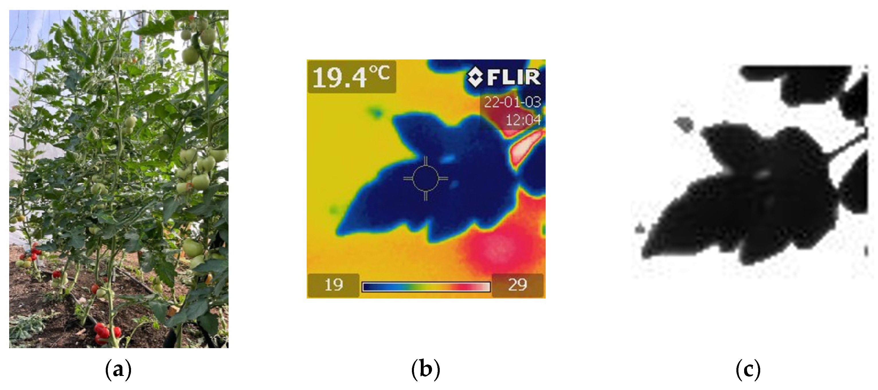
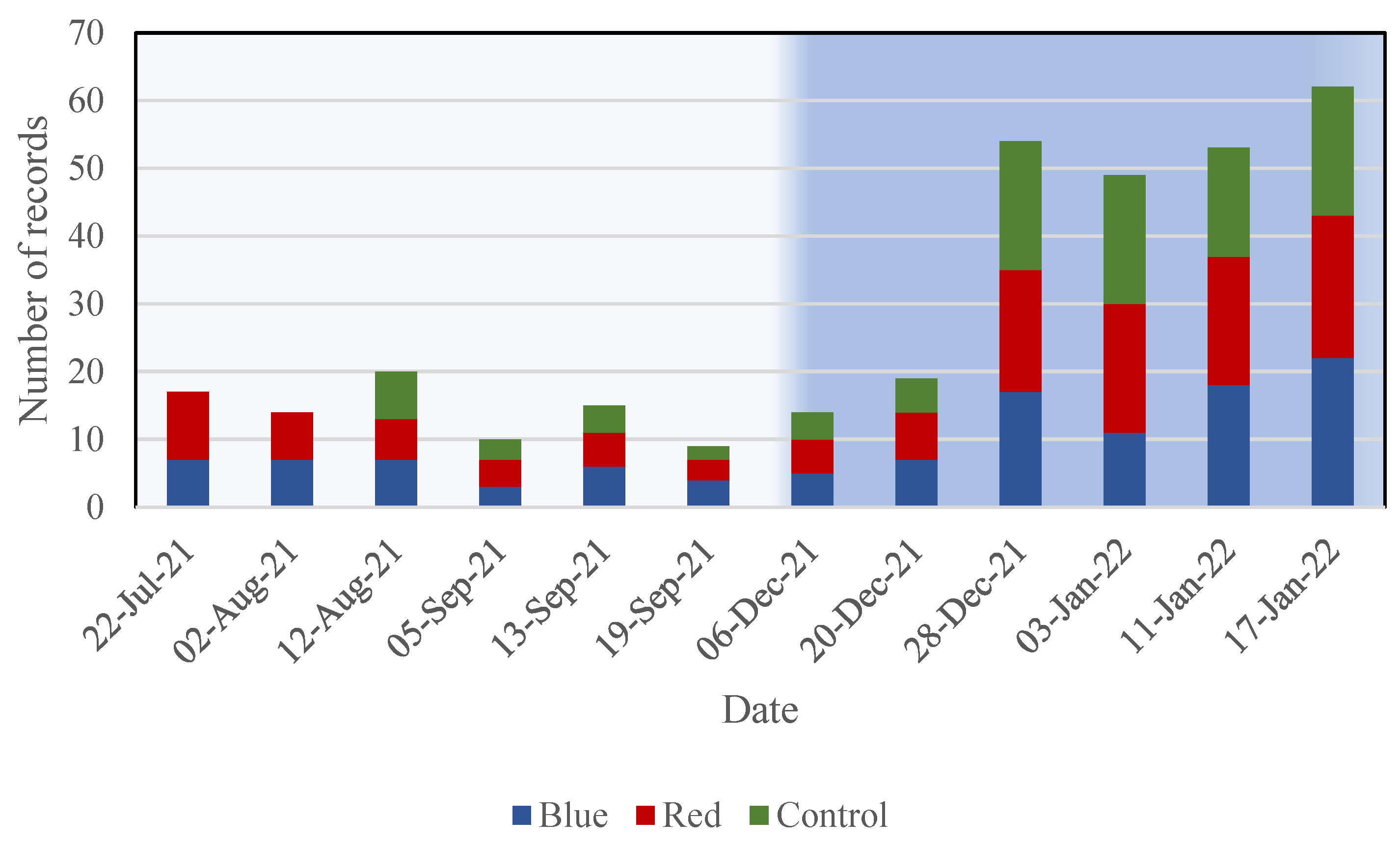
2.1. Experimental Work

The present study was done in three greenhouses during two growing seasons, examining the influence of OPV on plant growth. In two greenhouses, OPV modules were placed at gutter height above the canopy. One greenhouse had blue modules and the other red modules. The third greenhouse had no modules and served as a control. All three greenhouses had a gutter height of 3 m, with a 24 m2 floor area. In the summer season (6 June–7 October 2021), 71 ‘Maggie’ tomato plants were grown in each greenhouse. The plants were planted on 6 June 2021, arranged in two 4.7 m long double rows with a distance of 1.5 m between the centers of the double rows. The distance between each row in a pair was 0.5 m, with 0.4 m between adjacent plants in a row. According to regional recommendations, the plants were irrigated and fertilized by a drip irrigation system. On 7 October 2021, the summer season terminated. In the winter season (17 November 2021–17 January 2022), 65 ‘Maggie’ tomato plants were grown in each greenhouse. They were planted on 17 November 2021, and arranged similarly to the summer season.
The air temperature and relative humidity inside each greenhouse were measured at the center by three aspirated units that were placed at different heights (see Table 1). The incoming solar radiation into each greenhouse was measured by a pyranometer (LI-200R Li COR Inc., Lincoln, NE, USA) located about 2 m from the south-east corner at the top of the canopy. A meteorological station was placed near the greenhouses to measure the ambient conditions. The meteorological station measured the wind speed and direction, the dry and wet bulb air temperatures the global solar radiation (LI-200R Li COR Inc., Lincoln, NE, USA and CMP3, Kipp & Zonen, Delft, The Netherlands), and the diffuse radiation (CMP3, Kipp & Zonen, Delft, The Netherlands) using a shadowed pyranometer. Table 1 summarizes all sensors used in the experiments. Data from all four systems (three greenhouses and the meteorological station) were collected every 15 s. Average values were recorded every 10 min on three CR1000 and one CR6 (Campbell Scientific, Logan, UT, USA) data loggers. Table 2 and Table 3 summarize the climatic values measured by the meteorological and greenhouse systems, respectively, from both growing seasons.
LT estimation was performed based on sensors installed in the greenhouses and data from a meteorological station adjacent to the greenhouses.
The LT of 20–28 randomly selected plants in each greenhouse was measured manually using a thermal camera (FLIR i5, Wilsonville, Ore. USA) with an imaging emissivity of 0.95. The camera’s temperature range is −20 °C to 250 °C with an accuracy of ±2%. Each image was captured using 80 pixels. Every image captured one leaf at a time while placing a notebook behind the leaf to cancel the influence of the background radiation on the measurements. Moreover, the leaves were selected from both the top and bottom of each selected plant to obtain a good estimate of the average foliage temperature in which leaves at the top are exposed to direct sun radiation and at the bottom are shaded (Figure 1a). Images were also taken from both the east and west sides of each row of plants to cancel the effect of row orientation.
Every image was exported to ThermaCAM Researcher Professional software and saved as a Matlab file. The images were cropped in Matlab code to calculate the average temperature of the captured leaf while neglecting the non-relevant parts in the frame (Figure 1b,c). Eventually, the average of all images was calculated per greenhouse for comparison among the greenhouses.
Since the thermal images were collected manually, the times at which the images were collected during the day were not regular—the opposite of the situation with the data collected by the data loggers. In the case of capturing multiple images in the same minute, the LT is considered to be the average temperature from all images taken in that particular minute (hereafter referred to as the record). Since the average values from all sensors in each greenhouse were recorded every 10 min, these data were interpolated using the ‘Spline’ method to obtain a data resolution of one minute and a better fit of data collected by the data logger to the data obtained from thermal images.
Each column in Figure 2 represents the total number of records obtained in the three greenhouses from both growing seasons. As shown in Figure 2, most images were captured between 10:13 and 10:42, with later images captured until 13:00 p.m.
The number of thermal images taken in each greenhouse during the winter growing season was higher than in the summer to allow a larger database. Moreover, since it was realized that multiple images from the same minute need to be averaged, which reduced the number of records, the duration of capturing thermal images was extended during the winter season to gain more records. In the control greenhouse, sensors were installed on 2 August 2021, later than in the other two greenhouses. Thus, the analysis does not consider the thermal images taken before 2 August 2021 (Figure 3, green column is absent before 12 August).

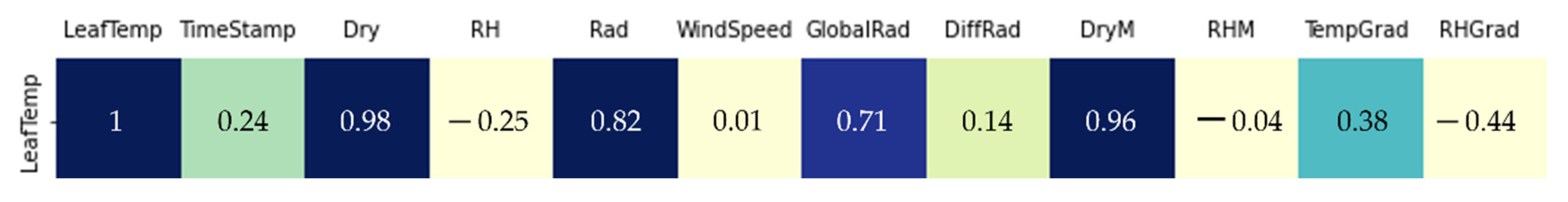
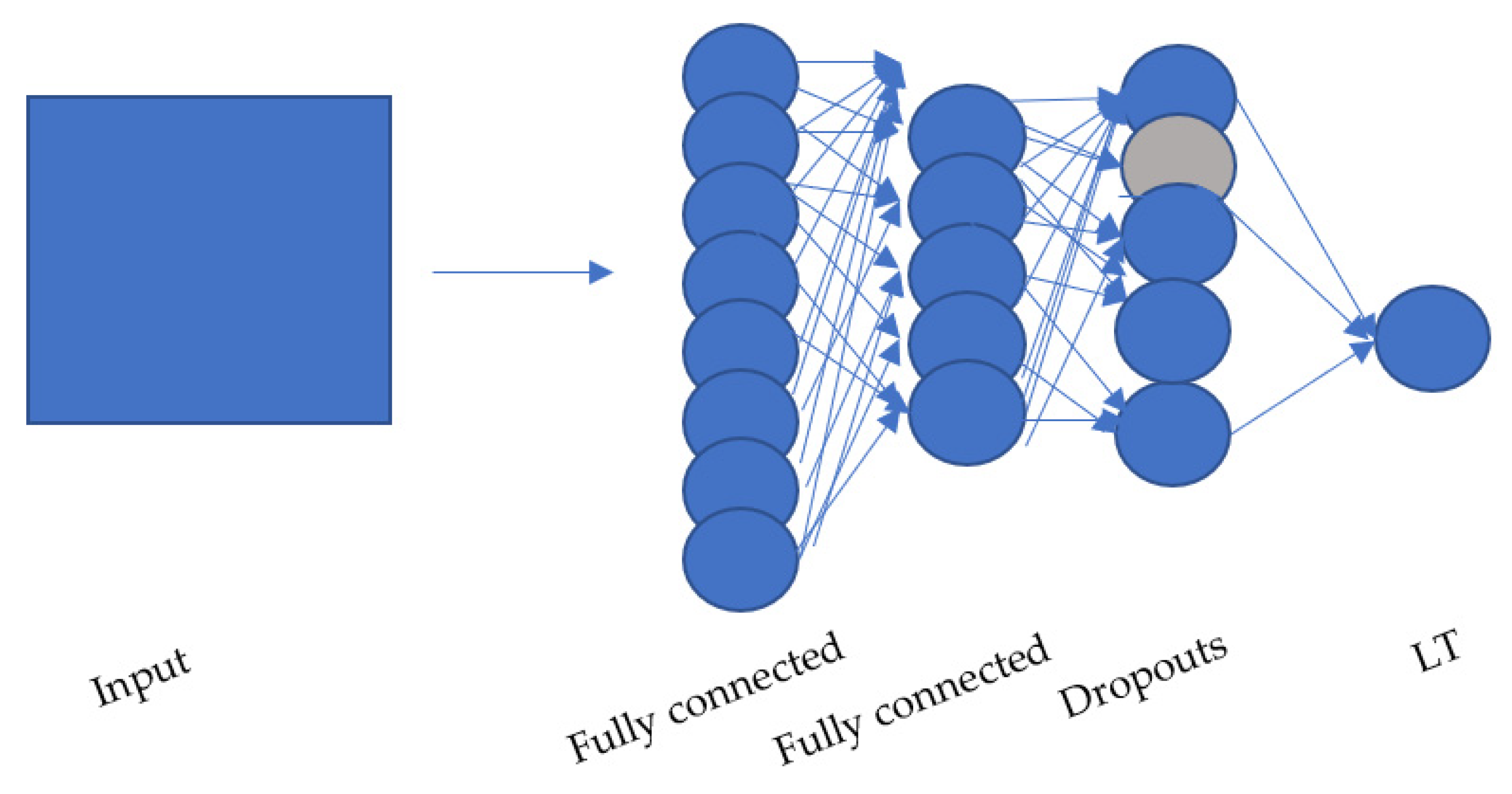
2.2. Methods Used in the Models
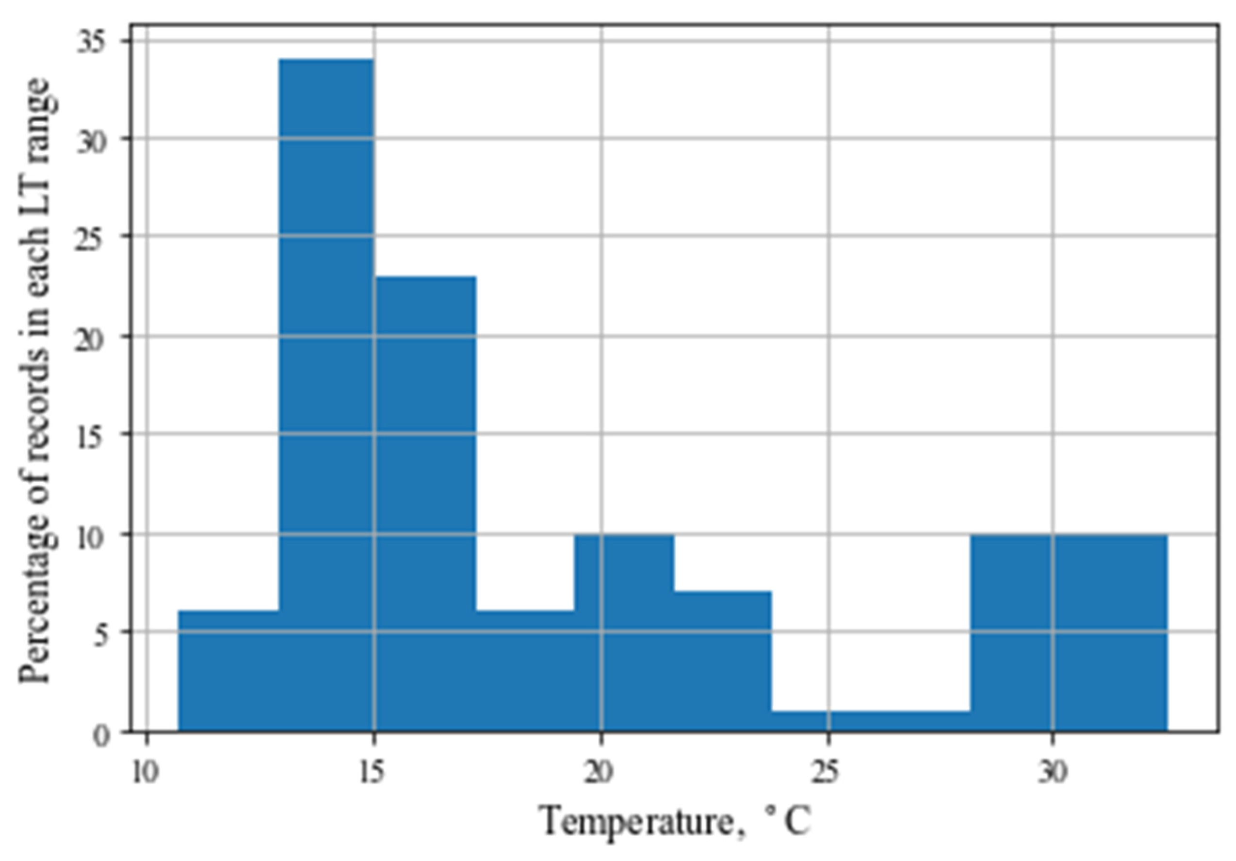
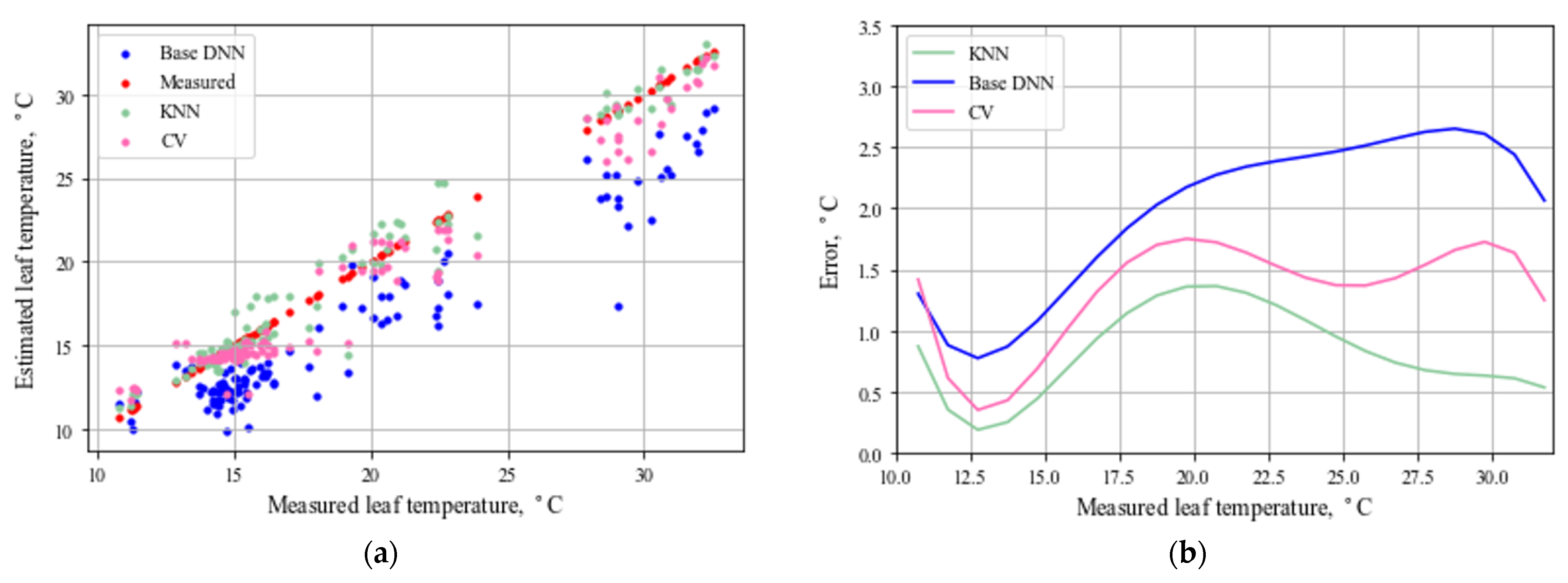
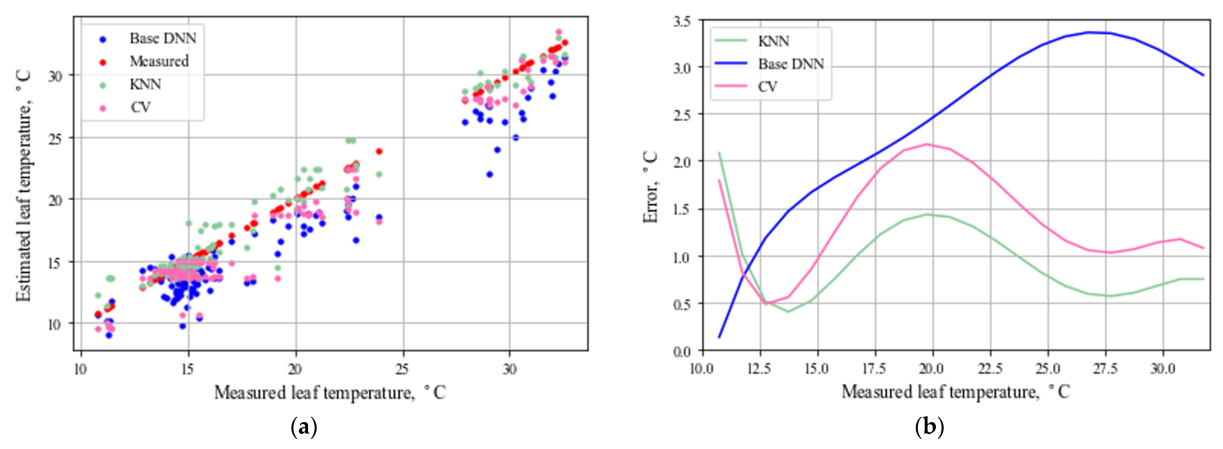
This study aims to develop a model which estimates LT based on easily measured parameters (inside each greenhouse and by a meteorologic station situated near the greenhouses). Furthermore, a comparison is made among one ML and two DNN models with regard to evaluating LT based on related features.
The main difference between the two DNN models is the method that was used to train the models which resulted in a different division into sub-sets. The first DNN model (hereafter referred to as BASE) used 75% of the entire data set for training and was evaluated by estimating LT using the remaining 25% of the data set, as suggested in [23]. On the other hand, the second model, the cross-validation (CV) model, was trained using 55% of the whole data set. Before testing the model, it was validated by cross-validation method using 20% of the whole data set. Eventually, the CV model was evaluated by estimating LT using the remaining 25% of the records.
To achieve a fair comparison between the BASE and CV models, both were trained with batch sizes of 512 over 1000 epochs. As the data are tabular, the two DNN models were compared to the KNN ML model with three neighbors, which was found (in a preliminary study we conducted) to produce the best results for LT estimation compared to five and seven neighbors. The KNN model, similar to the BASE model, used 75% of the data set for training and the remaining 25% for testing its LT estimation.
The BASE model architecture is based on [24]. In this model, which is summarized in Table 4 and described in Figure A1 in Appendix A, a sequential model containing six layers was established to evaluate LT using the Python Keras library. The first layer was the input layer, which received the training matrix. Thereafter, two one-dimensional convolutional layers were added to capture possible time-series patterns, using 64 filters of 5-length in each convolutional layer, padded with zeros when needed. Following the convolutional layers were two fully-connected layers with 10 and 1 neurons, respectively, which means each neuron in the fully-connected layer receives input from all neurons of its previous layer. In addition, 50% dropouts were added to avoid overfitting, which ignores randomly-selected neurons during model training. The best results of the BASE model were achieved by RELU activation functions in each layer and by a weighted initialization of a normal distribution. Eventually, the model was compiled using the ADAM optimizer.
Since the BASE model was created based on another estimation problem, with other features and limitations, it was suggested to compare the BASE model to other DNN models. Since the model’s goal is to estimate tomato LT in greenhouses at a specific time, rather than estimating the change in LT with time, the CV model was initiated without convolutional layers as detailed in Table 4 and in Figure A2 in Appendix A. Since the data are tabular, it was decided to use only fully-connected layers, of 15, 10, and 1 neurons, to estimate the LT. To avoid overfitting in this model as well, it was decided to use 25% dropouts in this architecture. Similar to the BASE model, the CV model contained RELU activation functions and was compiled using the ADAM optimizer.

3. Results

The performance of each model (Base, CV, and KNN) was evaluated using two methods, the root-mean-square error (RMSE) and absolute error (Err), and the Pearson correlation coefficient (R2), given by Equation (1), Equation (2), and Equation (3), respectively.
R M S E = 1 N i = 1 N ( Y t r u e i Y p r e d i c t e d i ) 2
E r r = m e a n ( | Y ¯ t r u e Y ¯ p r e d i c t e d | )
R 2 = σ Y t r u e Y p r e d i c t e d σ Y t r u e σ Y p r e d i c t e d
Table 5 shows the Err and RMSE values obtained with each model. It reveals that the KNN model had the best LT estimation, with an Err of 0.69 °C, while the CV and BASE models predicted LT with an Err of 0.93 °C and 1.76 °C, respectively. Similarly, the best RMSE values were obtained with the KNN model, 1.01 °C, followed by the CV and BASE models with 1.29 °C and 2.27 °C, respectively.
The R2 values for all three estimation methods were relatively similar and indicated a high correlation with the measured LT. Again, KNN seems to be the most accurate method with the highest R2 value.
Although this work deals with tomato cultivars in a greenhouse growing method, it appears to have a similar RMSE accuracy to the KNN model compared with the NN which predicted ‘Syrah’ cultivar LT [16]. However, the KNN Err was lower by 0.13 °C than the ‘Syrah’ NN Err. Tomato LT estimation was also conducted by linear regression on a greenhouse energy balance model [8]. Compared to this method, both the KNN and CV R2 had a higher correlation with the measured LT than that achieved by linear regression.
Generally, an error of 0.7 °C can be considered large in greenhouse energy balance calculations, which depend, among other parameters, on the difference between greenhouse air and foliage temperatures. However, it is noticed that errors with thermocouple sensors are about ±0.5 °C, as indicated in Table 1. Thus, an improved KNN module might be accurate as a thermocouple.
The size of the training and test data sets make a major contribution to a model’s accuracy, but the data distribution in the temperature range also affects the accuracy. The segmentation into training and test subsets was conducted by shuffling the data and dividing them according to desired subsets ratios. Figure 4 shows the histogram of the resulting test data set, divided into 10 equal-width columns of about 1.7 degrees each in the range of 10.75–32.53 °C.
Since the data were mostly collected during the winter season, more than 50% of the test data appears to lie around 15 °C, and 20% around 30 °C.
Figure 5a reveals the predictions of each model concerning the measured leaf temperature. Since most of the test data are around 15 °C (as shown in Figure 4), Figure 5 displays the high sample concentration at this temperature compared to other temperatures. In addition, predictions at 15 °C seem closer to the measured values compared to 25 °C or 30 °C, where there are fewer samples. Moreover, Figure 5a shows that the CV and BASE models tend to predict lower temperature values than the KNN model, which mostly predicted higher temperatures than the experimental values. In order to investigate the models’ predictions as a function of the leaf temperature, every model prediction was fitted to an O(5) polynomial line. Finally, Figure 5b demonstrates the behavior of the models’ absolute Err values as a function of the experimental LT values. From Figure 5b, it can be observed that the BASE model’s performance was inferior to the other models throughout the LT range. The CV and KNN had very similar errors between 13 and 20 °C. In addition, the Err values of the KNN model decreased at temperatures higher than 20 °C, while the Err values of the CV model remained relatively constant.
Since LT estimation is affected by a model’s features, the correlation between LT and every feature was tested.
Figure 6 shows the Pearson linear correlation between the values of each feature and the leaf temperature value. A darker color represents a higher correlation. This figure shows that the radiation, dry temperature, and vertical temperature gradients inside the greenhouses and the dry temperature and global radiation measured by the meteorological station have a high correlation, or impact, on the leaf temperature with a correlation coefficient higher than 0.7. Since it is common to use as few features as possible, especially for relatively small databases, each model was evaluated with the highly correlated features only. Since linear correlation was evaluated, the negative correlation factor indicates features that tend to move in an opposite direction to LT.
A comparison between the ‘full features’ model and the ‘high-correlated’ model (Table 6) shows that the ‘full features’ model has a higher accuracy. The Err of the ‘full features’ model was lower by 19, 26, and 16% than the ‘high-correlated’ model in the BASE, CV, and KNN models, respectively. Concerning the RMSE, the ‘full features’ model was lower by 10, 26, and 12% than the ‘high-correlated’ model, respectively. These differences between the ‘full features’ and ‘high-correlated’ models are relatively small, considering the contingency that the data are shuffled when separated into test and training subsets. Using all available data as model features seems necessary, especially with the CV model, which is the most affected. Minor changes in R2 were observed between full features results and high-correlated features results with KNN.
Figure 7 shows the high-correlated model performance as a function of the leaf temperature. Compared to Figure 5b, it seems to have a roughly similar Err behavior to the KNN model, which differs locally at a leaf temperature of 12 °C by 1 °C, but retains about the same accuracy as the ‘full features’ model throughout the leaf temperature range. The BASE ‘high-correlated’ model behaves similarly to the ‘full-features’ model but reaches a higher Err value of 3.7 °C at an LT of 26 °C, while the ‘full-features’ model retrieves an error of 3.2 °C. Running the ‘high-correlated’ model affected the CV model the most, with an Err of 2 °C at an LT of 20 °C, while the ‘full-features’ model had an Err of 1.5 °C. However, the CV model could improve at temperatures higher than 20 °C and reduce the Err to 1 °C, while the ‘full-features’ CV model retained a constant Err of 1.5 °C. Similar to the observation in Figure 5, the trend of the CV and BASE models to predict lower values than the KNN is also reflected in the ‘high-correlated’ models (Figure 7).

4. Conclusions

Leaf temperature is an essential parameter to track given that it affects plant and disease development and yield. This study compares the leaf temperatures predicted by two DNN models and an ML model using measured leaf temperatures obtained by a thermal camera in experimental greenhouses.
The three models were trained based on easily measured parameters in greenhouses and a nearby meteorological station. The results obtained with the KNN model are encouraging, with an average error of 0.7 °C. Thus, this model might be a good alternative to conventional leaf temperature measurements. With the average error of the CV model reported as 0.93 °C, it appears that—given enough data are collected—the CV model predictions could reach the same accuracy as those of the KNN. On the other hand, the BASE model was the least accurate model compared to the other models, with an average error of 2.1 °C. Moreover, the BASE and CV models are more complex than the KNN; therefore, these models require more computational resources and running time.
Training the models on only the ‘high-correlated’ features showed a lower performance—mainly with the DNN models which, unlike the ML model, performed similarly to the ‘full-features’ model. The accuracy of the BASE model decreased throughout the range of investigated LT, while the CV model accuracy showed a higher dependence on the amount of data at each LT. Additionally, in both ‘full-features’ and ‘high-correlated’ features predictions, the CV model had better LT estimations than the BASE model. The CV ‘high-correlated’ model had a better accuracy than the ‘full-features’ models when more data were available. This is a sign that, with CV, the quality of the features may be more significant than the number of features.
The present work showed that ML and DNN (CV) networks, based on greenhouse microclimate and meteorological data, can successfully estimate the average foliage temperature of a tomato crop. This finding can decrease the need for purchasing expensive measuring equipment such as a high-resolution thermal camera or damaging the plants when thermocouples are attached to the leaves.

Author Contributions

Conceptualization, R.G. and M.T.; Methodology, R.G.; Software, R.G.; Validation, R.G. and M.T.; Formal Analysis, R.G. and M.T.; Investigation, R.G., M.T., S.O. and A.L. (Asher Levi); Resources, M.T.; Data Curation, R.G., M.T., S.O. and A.L. (Asher Levi); Writing—Original Draft Preparation, R.G. and M.T.; Writing—Review & Editing, M.T. and A.L. (Avi Levy); Visualization, R.G. and M.T.; Supervision, M.T. and A.L. (Avi Levy); Project Administration, M.T. and A.L. (Avi Levy); Funding Acquisition, M.T. All authors have read and agreed to the published version of the manuscript.

Funding

This research was funded by the Israeli Ministry of Energy, grant number 220-11-057.

Institutional Review Board Statement

Not applicable.

Informed Consent Statement

Not applicable.

Acknowledgments

The authors thank Helena Vitoshkin, Eviathar Ziffer, Ibrahim Yehia, Esther Magadley, Roni Amir, Victor Alchanati, Farhad Geoola, and Eyal Ben Zion for the help with experiments and data analysis.

Conflicts of Interest

The authors declare no conflict of interest.

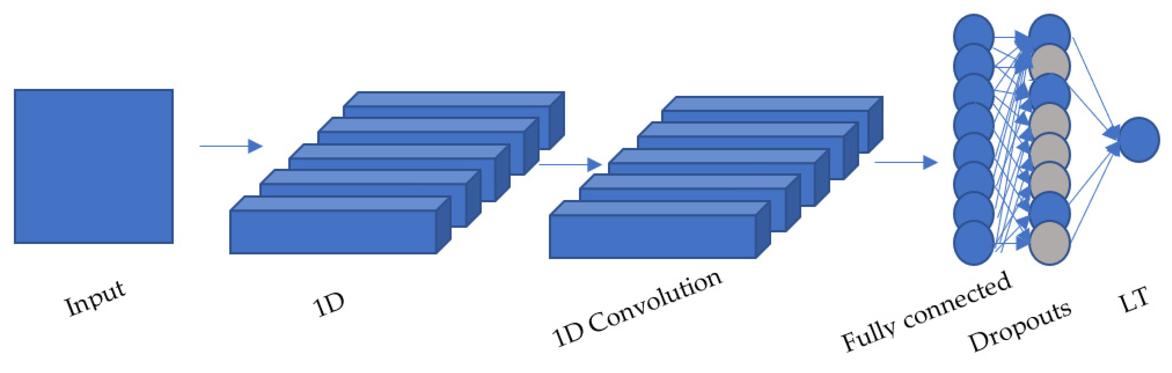
Appendix A. DNN Model Diagrams

Figure A1. Base model structure.
Agriculture 12 01034 g0a1
Figure A2. CV model structure.
Agriculture 12 01034 g0a2

References

  1. Gutschick, V. Leaf energy balance: Basics, and modeling from leaves to canopies. Canopy Photosynth. Basics Appl. 2016, 42, 23–58. [Google Scholar]
  2. Urban, J.; Ingwers, W.M.; McGuire, M.A.; Teskey, R.O. Increase in leaf temperature opens stomata and decouples net photosynthesis from stomatal conductance in Pinus taeda and Populus deltoides x nigra. J. Exp. Bot. 2017, 68, 1757–1767. [Google Scholar] [CrossRef] [PubMed] [Green Version]
  3. Vijayakumar, A.; Shaji, S.; Beena, R.; Sarada, S.; Sajitha Rani, T.; Stephen, R.; Manju, R.V.; Viji, M.M. High temperature induced changes in quality and yield parameters of tomato (Solanum lycopersicum L.) and similarity coefficients among genotypes using SSR markers. Heliyon 2021, 7, e05988. [Google Scholar] [CrossRef] [PubMed]
  4. Niu, G.; Kozai, T.; Sabeh, N. Physical environmental factors and their properties. Plant Fact. 2020, 11, 185–195. [Google Scholar]
  5. Seginer, I. Alternative design formulae for the ventilation rate of greenhouses. J. Agric. Engng Res. 1997, 68, 355–365. [Google Scholar] [CrossRef]
  6. Stanghellini, C. Transpiration of Greenhouse Crops: An Aid to Climate Management. Ph.D. Thesis, Agriculture University Wageningen, Wageningen, The Netherlands, 1987; 150p. [Google Scholar]
  7. Papadakis, G.; Frangondakis, A.; Kyritsis, S. Experimental investigation and modelling of heat and mass transfer between a tomato crop and the greenhouse environment. J. Agric. Engng. Res. 1994, 57, 217–227. [Google Scholar] [CrossRef]
  8. Wang, S.; Deltour, J. An experimental model for leaf temperature of greenhouse-growm tomato. Int. Soc. Hortic. Sci. 2021, 491, 101–106. [Google Scholar]
  9. Yu, L.; Wang, W.; Zhang, X.; Zheng, W. A Review on leaf temperature sensor: Measurement Methods and Application. Comput. Comput. Technol. Agric. IX 2016, 478, 216–230. [Google Scholar]
  10. Tarnopolsky, M.; Seginer, I. Leaf temperature error from heat conduction along thermocouple wires. Agric. For. Meteorol. 1999, 93, 185–194. [Google Scholar] [CrossRef]
  11. Canopy Temperature and Its Measurement by the Hand-Held Infrared Thermometer in the Field. Available online: https://plantstress.com/leaf-canopy-temperature (accessed on 10 May 2022).
  12. Leigh, A.; Close, D.J.; Ball, C.M.; Siebke, K.; Nicotra, N.B. Leaf cooling curves: Measuring leaf temperature in sunlight. Funct. Plant Biol. 2006, 33, 515–519. [Google Scholar] [CrossRef] [PubMed]
  13. Dariouchy, A.; Aassif, E.; Lekouch, K.; Bouirden, L.; Maze, G. Prediction of the intern parameters tomato greenhouse in a semi-arid area using a time-series model of artificial neural networks. Measurement 2009, 42, 456–463. [Google Scholar] [CrossRef]
  14. Linker, R.; Seginer, I.; Gutman, P.O. Optimal CO2 control in a greenhouse modeled with neural networks. Comput. Electron. Agric. 1998, 19, 289–310. [Google Scholar] [CrossRef]
  15. Hu, H.-G.; Xu, L.-H.; Wei, R.-H.; Zhu, B.-K. RBF network based nonlinear model reference adaptive PD controller design for greenhouse climate. Int. J. Adv. Comput. Technol. 2011, 3, 357–366. [Google Scholar]
  16. King, B.A.; Shellie, K.C. Evaluation of neural network modeling to predict non-water-stressed leaf temperature in wine grape for calculation of crop water stress index. Agric. Water Manag. 2016, 167, 38–52. [Google Scholar] [CrossRef]
  17. Patil, R.R.; Kumar, S.; Rani, R. Comparison of artificial intelligence algorithms in plant disease prediction, Revue d’Intelligence Artificielle. Int. Inf. Eng. Technol. Assoc. 2022, 36, 185–193. [Google Scholar]
  18. Kaur, P.; Harnal, S.; Tiwari, R.; Upadhyay, S.; Bhatia, S.; Mashat, A.; Alabdali, A.M. Recognition of leaf disease using hybrid convolutional neural network by applying feature reduction. Sensors 2022, 22, 575. [Google Scholar] [CrossRef] [PubMed]
  19. Ramana, K.; Aluvala, R.; Kumar, M.R.; Nagaraja, G.; Krishna, A.V.; Nagendra, P. Leaf disease classification in smart agriculture using deep neural network architecture and IoT. J. Circuits Syst. Comput. 2022, 31, 2240004. [Google Scholar] [CrossRef]
  20. Li, L.; Li, W.; Ma, D.; Yang, C.; Meng, F. Prediction model of transpiration of greenhouse tomato based on LSTM. Nongye Jixie Xuebao/Trans. Chin. Soc. Agric. Mach. 2021, 52, 369–376. [Google Scholar]
  21. Qu, Y.; Clausen, A.; Jørgensen, B.N. Net photosynthesis prediction by deep learning for commercial greenhouse production. In Proceedings of the INES 2021—IEEE 25th International Conference on Intelligent Engineering Systems, Budapest, Hungary, 7–9 July 2021; Volume 9512919, pp. 139–144. [Google Scholar]
  22. Wang, L.; Wang, P.; Liang, S.; Qi, X.; Li, L.; Xu, L. Monitoring maize growth conditions by training a BP neural network with remotely sensed vegetation temperature condition index and leaf area index. Comput. Electron. Agric. 2019, 160, 82–90. [Google Scholar] [CrossRef]
  23. How Do I Know Which Test Train to Split? Available online: https://it-qa.com/how-do-i-know-which-test-train-to-split/ (accessed on 10 May 2022).
  24. Manikumri, N.; Vinodhini, G.; Murugappan, A. Modeling of reference evapotranspiration using climatic parameters for irrigation scheduling using machine learning with limited data. ISH J. Hydraul. Eng. 2021, 28, 272–281. [Google Scholar]
Figure 1. Images of a tomato plant and leaf: (a) leaves exposed to incoming solar radiation at multiple sections of a plant and different directions, (b) thermal image, (c) processed thermal image.
Agriculture 12 01034 g001
Figure 2. Total number of records (each record is an average of LT values measured by a thermal camera at a particular minute) from all three greenhouses at different hours of the day (as indicated in the x-axis). Data of summer and winter growing seasons, from 22 July to 19 September 2021, and 6 December 2021 to 17 January 2022, respectively.
Agriculture 12 01034 g002
Figure 3. Number of records per day, divided stacked by greenhouse. Data of summer and winter growing seasons, from 22 July to 19 September 2021 (light blue background) and 6 December 2021 to 17 January 2022 (darker background), respectively.
Agriculture 12 01034 g003
Figure 4. Histogram of the test data set.
Agriculture 12 01034 g004
Figure 5. Leaf temperature and errors in estimation: (a) comparison between measured and predicted temperature; and (b) each model error as a function of the measured value.
Agriculture 12 01034 g005
Figure 6. Correlation between leaf temperate and the different features. Darker color represents a higher correlation. Values indicate the correlation coefficients.
Agriculture 12 01034 g006
Figure 7. Using high-correlated features: (a) KNN, BASE, and CV leaf temperature predictions versus the measured values; and (b) each model error as a function of the measured values.
Agriculture 12 01034 g007
Table 1. System of sensors in the greenhouses (GH) and in the meteorological station (M).
Sensor2D Sonic Anemometer (Windsonic, Gill, UK)Dry and Wet Bulb (Type T Thermocouples)Pyranometer (LI-COR LI-200SZ, LI-200R)Global Sun Radiation (CMP3)Diffuse Sun Radiation
(CMP3)
Number of sensors13, in each GH
1 in M
1, in each GH
1 in M
11
Sensor locationM (at a height of 6 m)GH: 0.5, 1.4, and 2 m above the ground
M: about 4 m above ground
GH: at the top of the canopy in the southeastern side of the greenhouseM: at a height of about 6 mM: at a height of about 5 m
Sensor accuracy±2% at 12 ms−1±0.5 °C3%<20 Wm−2<20 Wm−2
Table 2. Climatic values from the meteorological station from summer (22 July to 19 September 2021) and winter (6 December 2021 to 17 January 2022) growing seasons.
SeasonDiffused Radiation
Wm−2
Global Radiation
Wm−2
Wind Speed
ms−1
Air Temperature
°C
RH
%
Summer140.57 ± 38.51866.77 ± 41.872.13 ± 0.5631.95 ± 1.6353.61 ± 11.99
Winter109.56 ± 48.45264.17 ± 218.741.79 ± 0.5814.48 ± 2.6354.17 ± 14.91
Table 3. Climatic values from greenhouses from summer (22 July to 19 September 2021) and winter (6 December 2021 to 17 January 2022) growing seasons.
GreenhouseSeasonRH Gradient,
%m−1
Temperature Gradient
°Cm−1
Radiation
Wm−2
RH
%
Air Temperature
°C
Red OPVSummer−7.22 ± 2.611.29 ± 0.46352.53 ± 78.0555.92 ± 6.3731.55 ± 1.24
Winter−4.19 ± 1.220.7 ± 0.34176.96 ± 99.5959.3 ± 15.3115.83 ± 3.22
Blue OPVSummer−7 ± 2.871.23 ± 0.83400.08 ± 64.2948.59 ± 5.5631.26 ± 1.34
Winter−4.99 ± 1.521.32 ± 0.88182.14 ± 114.3659.66 ± 15.5316.17 ± 3.44
ControlSummer−5.05 ± 5.140.84 ± 0.93542.6 ± 30.0657.41 ± 7.2733.81 ± 1.1
Winter−1.85 ± 0.720.57 ± 0.31197.83 ± 109.7361.19 ± 16.1815.57 ± 2.9
Table 4. Architecture of DNN models. The numbers in brackets represent the number of neurons used in the fully connected layers. The percentage in brackets represents the percentage of dropped neurons.
BASECV
1D convolutionFully-connected (15)
1D convolutionFully-connected (10)
Fully-connected (10)Dropouts (25%)
Dropouts (50%)Fully-connected (1)
Fully-connected (1)
Table 5. Models’ performances.
ParameterBASECVKNN
Err, °C1.760.930.69
RMSE, °C2.271.291.01
R20.960.980.99
Table 6. Models’ performances. White background—model evaluation using all features, gray background—model evaluation with high-correlated features.
ParameterBASECVKNN
Err, °C2.091.761.180.930.80.69
RMSE, °C2.512.271.631.291.131.01
R20.960.960.980.980.980.99
Publisher’s Note: MDPI stays neutral with regard to jurisdictional claims in published maps and institutional affiliations.

