Article

Genotype by Environment Interaction Analysis for Grain Yield of Wheat (Triticum aestivum (L.) em.Thell) Genotypes

1
ICAR—Indian Institute of Wheat and Barley Research, Karnal 132001, India
2
Department of Genetics & Plant Breeding, Chaudhary Charan Singh Haryana Agricultural University, Hisar 125004, India
3
Department of Molecular Biology, Biotechnology and Bioinformatics, Chaudhary Charan Singh Haryana Agricultural University, Hisar 125004, India
*
Author to whom correspondence should be addressed.
Agriculture 2022, 12(7), 1002; https://doi.org/10.3390/agriculture12071002
Submission received: 7 June 2022 / Revised: 27 June 2022 / Accepted: 7 July 2022 / Published: 11 July 2022
(This article belongs to the Special Issue High Yield Cultivation, Growth and Development Mechanism of Wheat)

Abstract

:
Genotype environment interaction and stability performance were investigated on grain yield per plot in eight environments during Rabi (here, rabi means that a crop has been grown in Rabi season: crops that are sown in winter and harvested in spring in the Indian subcontinent) 2019–2020 and 2020–2021 using 100 diverse wheat genotypes. Research was conducted at Chaudhary Charan Singh Haryana Agricultural University, Hisar, Haryana in India. The analysis of variance revealed that genotype, environment and their interaction had a highly significant effect on the yield as reflected in Eberhart and Russel model and The Eberhart and Russell model indicated the suitability of the genotypes WH 1142, PBW 661, PBW 475 and DBW 17 with high mean, bi > 1 and non-significant deviation from regression to favorable environment, whereas the genotypes UP 2660 and DBW 88 with high mean, bi < 1 and non-significant deviation from regression were found suitable for poor environment. The Additive Main Effects and Multipicative Interaction (AMMI) analysis of variance for grain yield per plot across the environments showed that 26.41% of the total variation was attributed to genotypic effects, 70.22% to environmental effects and 3.37% to genotype × environment interaction effects. AMMI biplot study indicated the genotypes PBW 750, DPW 621-50, WH 542, PBW 486, PBW 661 and WH 1192 stable across the environments as they did not exert strong interactive forces; hence, they were selected as potential candidates for possible release in the study areas. Furthermore, the which-won–where model indicated the adaptation of genotypes PBW 706, PBW 769, DBW 116, WH 1157, WH 789 and WH1186 to first mega-environment and genotypes DBW 16, WH 1152, WH 1105 and PBW 503 in the second. These genotypes could be utilized in breeding programs to improve grain yield in bread wheat and may be used as stable breeding material for commercial cultivation.

1. Introduction

Wheat is a staple food crop of many countries across the globe, including India, which plays an important role in nutritional as well as food security. Additionally, it is an industrial crop because the grain, along with stalk and chaff, serves as industrial raw materials, which are also used as mulch, construction material and animal bedding. It contains good nutrition profile with 12.1% protein, 1.8% lipids, 1.8% ash, 2.0% reducing sugars, 6.7% pentosans, 59.2% starch and 70% total carbohydrates and provides 314 Kcal/100 g of food [1]. In India, wheat was cultivated over 31.45 million hectares with a record production of 107.6 million tons during 2019–2020 [2]. It can be grown not only in tropical and sub-tropical zones but also in temperate zone and the cold tracts of the far north, even beyond the 600 North, Central Zone and Peninsular Zone due to its versatile genotype, which has wide adaptation to diverse agro-ecological conditions. There are many constraints in the breeding of wheat. Among them, droughts and high temperatures are the most important limiting factors for crop production in the world [3]. Yield instability in wheat under heat and moisture stress can be caused by accelerated phasic development, increase in respiration [4], reduction in photosynthesis [5] and inhibition of starch synthesis in developing kernels, which affects both grain setting and grain filling. With looming negative climate change impacts on crop productivity, there is a need to develop high buffering wheat genotypes that adapt to diverse environmental conditions—more productive and with more stable yield in changing climate conditions.
For the development of stable varieties, there must be a presence of large genetic diversity in the populations under study. From these populations, one can identify genotypes showing wide stability under different environmental conditions. This is performed by understanding the interaction of genotype with the environment [6]. Genotype × Environment Interaction (GEI) is a phenomenon related to the inconsistent performance under diverse environmental conditions, and it plays an important role in the performance of genotypes under different environments [7]. G × E interaction reduces the efficiency of selection and accuracy of varietal recommendation [8]. Due to this interaction of the genotype × environment, it is necessary to study the genotype in the environment interaction before introducing new high-yielding genotypes with high stability in different environments. To reveal patterns of G × E Interaction, several statistical methods have been developed, which are usually divided into two groups, parametric and non-parametric. The parametric methods themselves are divided into two groups: univariate and multivariate. Univariate methods include stability factor [9], a regression-based approach [10,11,12,13], whereas multivariate methods include the AMMI (Additive Main Effects and Multipicative Interaction) model [14] and Genotypic Main Effect plus Geotype by environment (GGE) biplot analysis [15]. Eberhart and Russell (1966) suggested that regression coefficient ‘b’ and deviation from regression coefficient ‘S2d’ might predict stable genotype. A cultivar with b = 1 and S2d = 0 might be stable across divergent environmental conditions [16]. In addition, additive main effects and multiplicative interaction (AMMI) analysis has been proved as a useful analytic approach for linear and non-linear response of genotypes over the environmental conditions [17], which combines ANOVA (with additive parameters) and principal component analysis (with multiplicative parameters) into a single analysis [18] and interprets multi-environment data structure in breeding programs [19]. It is also an effective tool to diagnose genotype environment interaction patterns graphically [20]. Furthermore, the GGE (genotype plus genotype by environment interaction) biplot procedure is an effective tool based on principal component analysis (PCA) to fully explore multi-environment trials (METs) by partitioning G + GE into principal components through singular value decomposition of environmentally centered yield data [21]. So, for the breeders to develop a variety suitable for different environments, the analysis of the stability of genotypes is the most important tool. In this study, 100 wheat genotypes were evaluated for grain yield across different environments to identify stable genotypes for general and specific adaptation in different sowing conditions and to estimate genotype × environment interaction and stability parameters.

2. Material and Methods

2.1. Field Experimentation

The field experiment was conducted in four environments viz. irrigated, rainfed, timely sown and terminal heat stress during two consecutive years of Rabi (here, Rabi means a crop that has been grown in the Rabi season: crops that are sown in winter and harvested in spring in the Indian subcontinent) 2019–2020 and 2020–2021 at Chaudhary Charan Singh Haryana Agricultural University, Hisar, Haryana, India. The field, in timely sowing conditions, was sown in the third week of November (18 November) to provide normal temperature to wheat crop in the reproductive and ripening stage. In the field of terminal heat stress, sowing was delayed by a month (4th week of December; 22 December) to provide higher temperature to wheat crop in the reproductive and ripening stage, which causes heat stress. Table 1 represents codes used for different production environments.

2.2. Plant Materials

The research was conducted with 100 wheat genotypes (Table 2) at research area, Wheat and Barley section, Department of Genetics & Plant Breeding, CCS Haryana Agricultural University, Hisar, India. The 100 wheat genotypes included in the experiment were chosen on the basis of previous yield data, and the samples include both old cultivars that were previously widely cultivated and newly bred genotypes having great importance for today’s wheat production.

2.3. Experimental Design and Layout

The experiment was laid out in a Randomized Block Design (RBD) with 3 rows of 2 m length each, in two replications. A row to row distance of 20 cm was maintained for both dates of sowing. The observations were recorded on five randomly selected competitive plants from each genotype in each replication.

2.4. Statistical Analysis

The combined analysis of variance of yield data over all environments, using genotype–environment interaction data for stability analysis using the Eberhart and Russell model (Table 3 and Table 4), AMMI model and GGE biplot analysis was performed with the help of INDOSTAT 8.1, Hyderabad, India and PB tools developed at IRRI, Philippines.
The AMMI model equation is:
Yij = μ + gi + ej + Σλnαinγjn + θij
where
Yij = mean yield of ith genotype in the jth environment
μ = general mean
gi = ith genotypic effect
ej = jth location effect
λn = eigen value of the Principal Component Axis n
αinγjn = ith genotype, jth environment Principle component analysis (PCA) scores for the PCA axis
θij = residual
n = number of PCA axes retained in the model.
The equation for Eberhart and Russell model is:
Yij = μi + βiIj + Sij
where
Yij = Mean of the ith variety at the jth environment
μi = Mean of ith variety over all environments
βi = The regression coefficient that measures the response of ith variety to varying environments
Sij = The deviation from regression of the ith variety at the jth environment
Ij = The environmental index obtained by subtracting the grand mean from the mean of all varieties at the jth environment
Simultaneous study of the genotype plus genotype–environment interaction was performed using GGE biplot, where GGE biplot used principal component consisting of a set of elite lines scores multiplied by environment scores, which gives a two-dimensional biplot.

3. Results

3.1. Eberhart and Russell Model

The genotype–environment interaction component (GEI) was elaborated by using the joint regression model of stability analysis [11]. The mean grain yield per plot among the genotypes ranged from 394.30 to 841.60, with an overall population mean of 576.27. PBW 729 gave the maximum grain yield per plant (841.6), whereas minimum grain yield per plot was observed in DBW 90 (394.3) (Table 5). Considering Eberhart and Russell’s model of analysis, significant differences were revealed by a pooled analysis of variance for both the main effects, genotypes and environments, as well as for interaction effects (Table 6). No genotype had bi = 1 and S2di = 0; however, some genotypes, HD 3086, DBW 16, PBW 527, PBW 528, PBW 502 and PBW 503, had bi values near to one, showing that most of these genotypes almost produced similar grain yield per plot under all the environments (Table 5). Genotypes WH 1142 (μ = 622, bi = 1.158**, S2di = −1135.98), PBW 661 (μ = 609.50, bi = 1.13**, S2di = −1299.38), PBW 475 (μ = 810.80, bi = 1.11*, S2di = −1056.61) and DBW 17 (μ = 606.70, bi = 1.10*, S2di = −1431.94) were observed to be stable in a rich (E5) environment (Table 5), whereas for genotypes UP 2660 (μ = 594.10, bi = 0.99**, S2di = 341.71) and DBW 88 (μ = 664.10, bi = 0.97*, S2di = 44.95), high means with lower bi values were detected. The lower values of bi indicate that these genotypes show more resistance to the unfavorable (E4) environment. The performance was unpredictable for the genotypes WH 1182, PBW 677, WH 1061, PBW 729, PBW 560, PBW 728 and PBW 721, as these genotypes had significant deviations from regression.

3.2. Environmental Indices

The environment index reveals the suitability of an environment at a particular location. Estimates of environment index can provide the basis for identifying the favorable environment for the expression of maximum potential of the genotype. The positive values of environment indices conclude the favorable environment for genotypes. As indicated by the environment index, E5 (260.03) showed highest yield and was found to be most favorable production environment (Table 7).

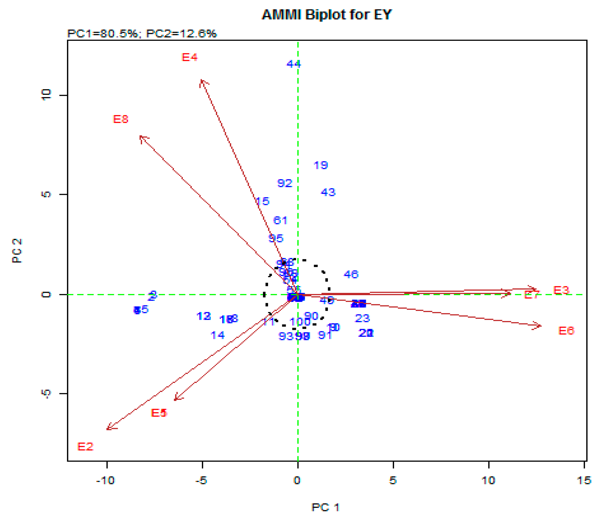
3.3. AMMI Biplot Analysis

G × E interaction study in multi-environment trials was also carried out by AMMI model to increase the reliability of the multi-location trial analysis. The results of the analysis of variance of the AMMI model revealed that grain yield is significantly (p < 0.001) affected by environment, genotype and genotype–environment interaction, which explained 70.22%, 26.41% and 3.37% of the occurred variation, respectively. Furthermore, it showed that two PC with significant differences cumulatively captured 93.14% of total GEI as the first principal component of AMMI, explaining 80.52% of the genotype–environment interaction, whereas the second principal component explained 12.62% of the genotype–environment interaction (Table 8).

3.4. The AMMI 1 Model

The AMMI biplot has the main effect as grain yield per plot in the abscissa and the IPCA1 as the ordinate where the genotypes or environments that lie on the same vertical line have the same yield, and those that lie on the same horizontal line have the same interaction pattern. In the AMMI 1 biplot, the elite wheat genotypes PBW 750, DPW 621-50, WH 542, PBW 486, PBW 661 and WH 1192 are relatively stable genotypes in yield that are broadly adapted lines (Figure 1).
The wheat genotypes HD 2967, WH 1151, UP 2660, PBW 676, WH 1182, PBW 729, WH 1061, PBW 560, PBW 725 and PBW 721 are relatively unstable in yield because these lines are far from the origin and can be specifically adapted to particular environment. Especially, genotypes HD 2967, WH 1151, UP 2660 and PBW 676 were likely to perform better in the E6 environment, whereas the genotypes WH 1182 and PBW 729 were identified as specially adapted to environments E1 and E5, respectively. E8 was the most responsive environment for genotypes WH 1061, PBW 560, PBW 725 and PBW 721 (Figure 1).

3.5. The AMMI2 Model

In AMMI2 biplot, the Interaction Principal Component Axes 1(IPCA1) and Interaction Principal Component Axes 2 (IPCA2) scores are reported as the representation of the stability of the lines across the environment; that is, the lines with the least PC scores have high stability and vice versa, i.e., the more IPCA scores that approximate to zero, the more stable the genotypes are across all the locations. The environments E1 and E5 had comparatively short spokes, and they did not exert strong interactive forces, while environments E2, E3, E4, E6, E7 and E8 had long spoke exert strong interaction (Figure 2). Similarly, genotypes WH 1158, WH 1164 and PBW 726 were near the origin, so they were non-sensitive to environmental interactive forces, while genotypes PBW 706, WH 1063, PBW 343 and PBW 762 were away from the zero line, so they were the most responsive. In this case, the best-adapted genotype with respect to site E4 was WH 1063, whereas the genotypes WH 1152, PBW 752 and PBW 475 were tightly grouped in the sites E1, E2 and E5.

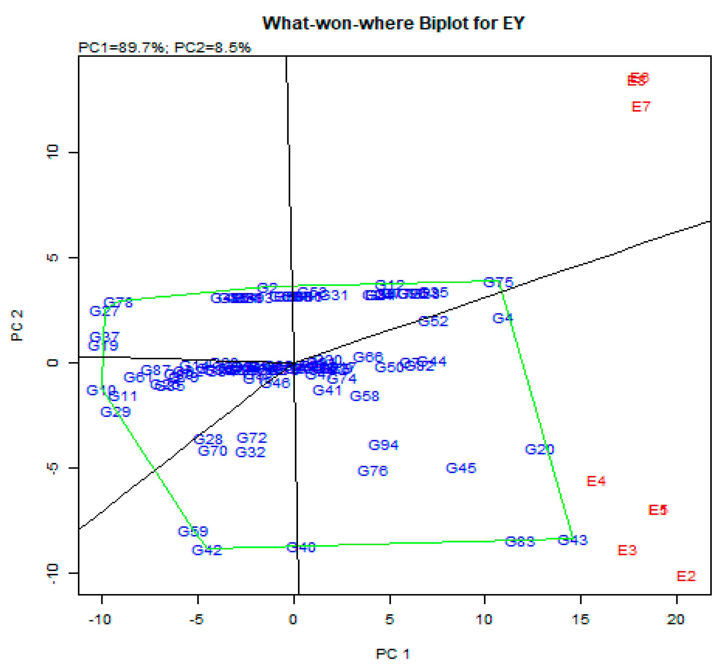
3.6. GGE Biplot Analysis

Which-Won-Where Model

GGE biplot analysis, the most effective way of summarizing the genotype and genotype–environment interaction of the dataset was used to identify the best line of each environment and assess the stability of the lines. The most attractive feature of GGE biplots is the polygon view, which addresses the ‘which-won-where’ pattern of multi environment data, in which there is a graphical representation of crossover GE interaction, mega-environment differentiation and specific genotype adaptation. The polygon is drawn by joining the genotypes located farthest from the origin, such that all other genotypes are included within the polygon. A genotype located at the edge is called a vertex genotype, and vertex genotypes were the most responsive. In this biplot, genotypes DPW 621-50, DBW 16, PBW 88 and PBW 706 were the most responsive genotypes. The equality line divides the graph into six sectors, and eight environments were retained in two sectors and partitioned into two mega-environments, one with E1, E2, E3, E4 and E5, and the second with E6, E7 and E8 (Figure 3). In the first mega-environment, the genotypes PBW 706, PBW 769, DBW 116, WH 1157, WH 789 and WH1186 were the winning genotypes, and genotypes DBW 16, WH 1152, WH 1105 and PBW 503 were those in the second (Figure 3).

4. Discussion

A major goal of plant breeding programs is to increase stability and stabilize crop yield over a range of environments. The most appropriate methods include identifying desirable cultivars with high productivity genetic potential and testing wide adaptability to most conditions by multi-condition experiments in target environments. The results of pooled analysis of variance for stability as devised by Eberhart and Russell [11] and the AMMI model showed that variance due to genotypes and environments was significant for grain yield per plot, indicating that the performances of genotypes as well as the environments were different; the genotypes also had differential responses to the changes in the environmental conditions. Similar results were reported by Dhiwar et al. [22] and Attia et al. [23]. In this study, the four genotypes WH 1142, PBW 661, PBW 475 and DBW 17 had regression coefficients of 1.158, 1.13, 1.11 and 1.10 and were observed to be stable in the rich (E5) environment. According to the E-R model, a slope of >1.0 with high mean and non-significant squared deviation are suitable for a favorable environment [24]. Suresh and Munjal [25] found four genotypes, namely HD 3059, WH 1105, HTW 66 and WH 1124, with bi values significantly greater than 1 and with higher average productivity than the overall mean; these conditions are suitable for high input and timely sowing conditions.
It is interesting to note that no genotype was stable for grain yield; however, some genotypes, HD 3086, DBW 16, PBW 527, PBW 528, PBW 502 and PBW 503, almost produced a similar grain yield per plot under all the environments. Similar results were reported by Kumar et al. [26], who observed that the genotypes LOK-1, NI-5439 and HUW-468 were found stable across the environments with high mean value, bi values close to 1 and non-significant deviation from regression. In this study, genotypes UP 2660 and DBW 88 were determined to be suitable for unfavorable environments, as genotypes with less than unity regression value and non-significant squared deviation indicate suitability for a poor environment [27]. The performance was unpredictable for genotypes WH 1182, PBW 677, WH 1061, PBW 729, PBW 560, PBW 728 and PBW 721 with significant squared deviation. For the genotypes exhibiting non-significant deviations from regression (S2di), their performance can be predicted well, as the genotypes are within the range of minimum deviation from regression [28].
The AMMI model explains the genotype–environment interaction [29], which is used for reliable yield estimates [30], and provides a base of better use for other models [19]. AMMI revealed that a major part of the variation in yield is explained by environment, which indicates that the environments were diverse. The results are line with the findings of Ljubičić et al. [31] and Hanif et al. [32].
The AMMI1 biplot analysis revealed variation due to the main effect (grain yield) and the interaction effect [33]. Genotypes and environments with IPCA1 scores close to zero were characterized with low interaction effects, being considered stable [34]. In this study, the wheat genotypes PBW 750, DPW 621-50, WH 542, PBW 486, PBW 661 and WH 1192 were identified as stable genotypes in yield, and the genotypes HD 2967, WH 1151, UP 2660, PBW 676, WH 1182, PBW 729, WH 1061, PBW 560, PBW 725 and PBW 721 were unstable. Similar to this research, Dabi et al. [35] also identified high-yielding and stable genotypes ETBW 9080, ETBW 9172, ETBW 9646, ETBW 9396, ETBW 9452, ETBW 9136 and ETBW 9139, inferring little interaction with the environment. Genotypes HD 2967, WH 1151, UP 2660 and PBW 676 far from the IPCA origin appeared to be adapted to a timely sown rainfed environment, whereas the genotypes WH 1182 and PBW 729 were specially adapted to a timely sown irrigated environment. Additionally, Bishwas et al. [36] identified the high-responsive genotypes of wheat in irrigated and heat-stressed environments. Especially, NL 1179 was specifically adapted to an irrigated environment, and Gautam, NL 1404 and NL 1381 were specifically adapted to a terminal heat-stressed environment.
An AMMI2 biplot was devised using genotypic and environmental scores (IPCA1 versus IPCA2 scores), providing a good explanation of the data pattern to interpret genotypic behaviors across different environments [37]. The IPCA 1 and IPCA 2 scores delineated the stability of the lines across the environment—that is, the lines with the least PC scores do not show an association with any environment, whereas a lower PC score means genotypes show specific adaptation to a particular environment [38]. In the present study, genotypes WH 1158, WH 1164 and PBW 726 were highly stable, while the genotypes PBW 706, WH 1063, PBW 343 and PBW 762 were the most responsive. According to the AMMI2 biplot, timely sown irrigated environment was determined as the most favorable environment, with the least interactive forces, and WH 1025 was highly adapted to this environment. Similarly, Attia et al. [23] concluded East Barrani as most favorable environment for all cultivars according to AMMI2 bi-plot and Sakha 94 was the superior cultivar in this environment. Similar results were further confirmed by Verma and Singh [17] while analyzing the stability of wheat genotypes by AMMI in the Peninsular Zone of India. Therefore, the above-mentioned genotypes were found most stable for grain yield and can be incorporated as breeding stocks in any future breeding programs aiming to produce high yielding lines of bread wheat.
The GGE biplot is a data visualization tool that allows an evaluation of environments due to the discriminative ability and representativeness of the GGE view, which is an advantage over the AMMI biplot analysis [39]. The GGE biplot analysis is the most effective way for a precise and useful interpretation of genotype–environment interactions as well as interrelationships among various test environments and genotypes and identifies the best line of each environment [40]. Genotypes and environments were analyzed together through the which-won-where model of the GGE-biplot. The vectors were connected furthest from the origin of the biplot, and a polygon was obtained. In this biplot, genotypes DPW 621-50, DBW 16, PBW 88 and PBW 706 were the most responsive genotypes, with crossover GE interaction, mega-environment differentiation and specific genotype adaptation [41]. These vertex genotypes were the most responsive, located at the greatest distance from the biplot origin [40]. The graph was then divided into six sectors, and eight environments were retained in two sectors and partitioned into two mega-environments, probably due to latitudinal and longitudinal differences [42]. Variation in the genotypic performance within environments indicated the strong influence of environments and the existence of a mega-environment [40,43,44].

5. Conclusions

This study indicated that genotype, environment and their interaction have a significant effect on the yield stability as per the Eberhart and Russell model, AMMI and GGE biplot. Further analysis of stability through the Eberhart and Russell model concluded that elite wheat genotypes WH 1142, PBW 661, PBW 475 and DBW 17 were specifically adapted to a timely sown irrigated environment during Rabi 2020–2021, whereas UP 2660 and DBW 88 were specifically adapted to late sown rainfed environment during Rabi 2019–2020. In this experiment, PBW 750, DPW 621-50, WH 542, PBW 486, PBW 661 and WH 1192 were found to be the most stable and high-yielding genotypes across all the test environments as per AMMI biplot. All in all, these genotypes can be used as high-yielding lines, which are stable too, and for farmers, WH 1142, PBW 661, PBW 475 and DBW 17 can be used for high yield with adaptability in a timely sown irrigated environment, whereas genotypes UP 2660 and DBW 88 were adapted to a late-sown rainfed environment. These genotypes need to be further tested in heat- and drought-stressed environments to ensure their performance over the years.

Author Contributions

V.G.: Conducting study and data collection; M.K.: Planning and guidance; V.S.: Field Resources; L.C.: Data curation; S.Y. and R.S. (Ravika Sheoran): Editing of manuscript; M.S.D.: Field planning; A.N.: Data analysis; K.L., N.G. and S.N.: Helped in data collection; R.S. (Rajat Sharma): Rough draft preparation. All authors have read and agreed to the published version of the manuscript.

Funding

This research received no external funding.

Institutional Review Board Statement

Not applicable.

Acknowledgments

The authors would like to express sincere thanks to CCSHAU, Hisar, Haryana for providing the facilities to accomplish this research work.

Conflicts of Interest

The authors declare that there are no conflict of interest.

References

  1. Singh, B.; Snehdeep, U.S.; Arya, C. Statistical assessment of rainfall trend and distribution on wheat yield in western Uttar Pradesh. In Proceedings of the Virtual National Conference on Strategic Reorientation for Climate Smart Agriculture (V-AGMET 2021), Ludhiana, India, 17–19 March 2021; Volume 2, p. 163. [Google Scholar]
  2. Anonymous (2021) Annual Report of Department of Agriculture, Cooperation & Farmers Welfare 2020–2021, Ministry of Agriculture & Farmers Welfare Government of India. Available online: www.agricoop.nic.in (accessed on 20 January 2022).
  3. Bocianowski, J.; Prażak, R. Genotype by year interaction for selected quantitative traits in hybrid lines of Triticum aestivum L. with Aegilops kotschyi Boiss. and Ae. variabilis Eig. using the additive main effects and multiplicative interaction model. Euphytica 2022, 218, 11. [Google Scholar] [CrossRef]
  4. Hassan, M.A.; Xiang, C.; Farooq, M.; Muhammad, N.; Yan, Z.; Hui, X.; Yuanyuan, K.; Bruno, A.K.; Lele, Z.; Jincai, L. Cold Stress in Wheat: Plant Acclimation Responses and Management Strategies. Front. Plant. Sci. 2021, 12, 676884. [Google Scholar] [CrossRef] [PubMed]
  5. Prasad, P.V.V.; Djanaguiraman, M.; Jagadish, S.V.K.; Ciampitti, I.A. Drought and high temperature stress and traits associated with tolerance. Sorghum A State Art Future Perspetives 2019, 58, 241–265. [Google Scholar]
  6. Regmi, D.; Poudel, M.R.; Bishwas, K.C.; Poudel, P.B. Yield Stability of Different Elite Wheat Lines under Drought and Irrigated Environments using AMMI and GGE Biplots. Int. J. Appl. Sci. Biotechnol. 2021, 9, 98–106. [Google Scholar] [CrossRef]
  7. Bhartiya, A.; Aditya, J.P.; Kumari, V.; Kishore, N.; Purwar, J.P.; Agrawal, A.; Kant, L. Stability analysis of soybean [Glycine max (L.) Merrill] genotypes under multi-environments rainfed condition of North Western Himalayan hills. Indian J. Genet. Plant Breed. 2018, 78, 342–347. [Google Scholar] [CrossRef]
  8. Crossa, J.; Cornelius, P.L. Sites regression and shifted multiplicative model clustering of cultivar trial sites under heterogeneity of error variances. Crop Sci. 1997, 37, 406–415. [Google Scholar] [CrossRef]
  9. Lewis, D. Gene-environment interaction: A relationship between dominance, heterosis, phenotypic stability and variability. Heredity 1954, 8, 333–356. [Google Scholar] [CrossRef] [Green Version]
  10. Finlay, K.W.; Wilkinson, G.N. The analysis of adaptation in a plant-breeding programme. Aust. J. Agric. Res. 1963, 14, 742–754. [Google Scholar] [CrossRef] [Green Version]
  11. Eberhart, S.A.; Russell, W.A. Stability Parameters for Comparing Varieties. Crop Sci. 1966, 6, 36–40. [Google Scholar] [CrossRef] [Green Version]
  12. Perkins, J.M.; Jinks, J.L. Environmental and genotype-environmental components of variability. Heredity 1968, 23, 339–356. [Google Scholar] [CrossRef] [Green Version]
  13. Freeman, G.H.; Perkins, J.M. Environmental and genotype environmental components of variability VIII. Relations Genotypes Grown Differ. Environ. Meas. These Environ. Hered. 1971, 27, 15. [Google Scholar]
  14. Gauch, H.G., Jr. Model selection and validation for yield trials with interaction. Biometrics 1988, 44, 705–715. [Google Scholar] [CrossRef]
  15. Yan, W.; Hunt, L.A.; Sheng, Q.; Szlavnics, Z. Cultivar evaluation and mega-environment investigation based on the GGE biplot. Crop Sci. 2000, 40, 597–605. [Google Scholar] [CrossRef]
  16. Awaad, H.A. Performance, adaptability and stability of promising bread wheat lines across different environments. In Mitigating Environmental Stresses for Agricultural Sustainability in Egypt; Springer: Cham, Switzerland, 2021; pp. 187–213. [Google Scholar] [CrossRef]
  17. Verma, A.; Singh, G.P. GxE Interactions Analysis of Wheat Genotypes Evaluated Under Peninsular Zone of the Country by AMMI Model. Am. J. Agric. For. 2021, 9, 29–36. [Google Scholar] [CrossRef]
  18. Gauch, H.G.; Zobel, R.W. Predictive and postdictive success of statistical analyses of yield trials. Theor. Appl. Genet. 1988, 76, 1–10. [Google Scholar] [CrossRef]
  19. Heidari, S.; Aziinezhad, R.; Haghparast, R. Yield stability analysis in advanced durum wheat genotypes by using AMMI and GGE biplot models under diverse environment. Indian J. Genet. Plant Breed. 2016, 76, 274–283. [Google Scholar] [CrossRef]
  20. Kumar, S.; Kumari, J.; Bansal, R.; Upadhyay, D.; Srivastava, A.; Rana, B.; Yadav, M.K.; Sengar, R.S.; Singh, A.K.; Singh, R. Multi-environmental evaluation of wheat genotypes for drought tolerance. Indian J. Genet. 2018, 78, 26–35. [Google Scholar] [CrossRef]
  21. Hagos, H.G.; Abay, F. AMMI and GGE biplot analysis of bread wheat genotypes in the northern part of Ethiopia. J. Plant. Breed. Genet. 2013, 1, 12–18. [Google Scholar]
  22. Dhiwar, K.; Sharma, D.J.; Agrawal, A.P.; Pandey, D. Stability analysis in wheat (Triticum aestivum L.). J. Pharmacogn. Phytochem. 2020, 9, 295–298. [Google Scholar]
  23. Abd El-Hammed Attia, M.; EL-Ghany, F.; El-Sadek, A.; Nawar, A.; Dessouky, A.; Shaalan, A. Genotype by environment interaction and yield stability in bread wheat cultivars under rainfed conditions. Sci. J. Agric. Sci. 2021, 3, 56–65. [Google Scholar] [CrossRef]
  24. Ibrahim, H.A.; Ibrahim, A.E.S.; Ali, K.A. Genotype by environment interaction and stability analyses of grain yield of selected maize (Zea mays L.) genotypes in eastern and central Sudan. Gezira J. Agric. Sci. 2021, 17, 294–312. [Google Scholar]
  25. Suresh, S.P.; Munjal, R. Selection of wheat genotypes under variable sowing conditions based on stability analysis. J. Cereal Res. 2020, 12, 109–113. [Google Scholar]
  26. Kumar, A.; Chand, P.; Thapa, R.S.; Singh, T. Assessment of stability performance and GXE interaction for yield and its attributing characters in bread wheat (Triticum aestivum L.). Electron. J. Plant Breed. 2021, 12, 235–241. [Google Scholar]
  27. Naheed, H.; Rahman, H.U. Stability Analysis of Bread Wheat Lines using Regression Models. Sarhad J. Agric. 2021, 37, 1450–1457. [Google Scholar] [CrossRef]
  28. Kant, S.; Lamba, R.A.S.; Arya, R.K.; Panwar, I.S. Effect of terminal heat stress on stability of yield and quality parameters in bread wheat in southwest Haryana. J. Wheat Res. 2014, 6, 64–73. [Google Scholar]
  29. Crossa, J.; Gauch, H.G.; Zobel, R.W. Additive main effects and multiplicative interaction analysis of two international maize cultivar trials. Crop Sci. 1990, 30, 493–500. [Google Scholar] [CrossRef]
  30. Zobel, R.W.; Wright, M.J.; Gauch, H.G., Jr. Statistical analysis of a yield trial. Agron. J. 1988, 80, 388–393. [Google Scholar] [CrossRef]
  31. Ljubičić, N.; Popović, V.; Ćirić, V.; Kostić, M.; Ivošević, B.; Popović, D.; Pandžić, M.; El Musafah, S.; Janković, S. Multivariate Interaction Analysis of Winter Wheat Grown in Environment of Limited Soil Conditions. Plants 2021, 10, 604. [Google Scholar] [CrossRef]
  32. Hanif, U.; Gul, A.; Amir, R.; Munir, F.; Sorrells, M.E.; Gauch, H.G.; Mahmood, Z.; Subhani, A.; Imtiaz, M.; Alipour, H.; et al. Genetic gain and G X E interaction in bread wheat cultivars representing 105 years of breeding in Pakistan. Crop Sci. 2022, 62, 178–191. [Google Scholar] [CrossRef]
  33. Anuada, A.M.; Cruz, P.C.S.; De Guzman, L.E.P.; Sanchez, P.B. Grain yield variability and stability of corn varieties in rainfed areas in the Philippines. J. Crop Sci. Biotechnol. 2022, 25, 133–147. [Google Scholar] [CrossRef]
  34. Ali, M.B.; El-Sadek, A.N. Ammi Biplot Analysis of Genotype × environment interaction in wheat in Egypt. Egypt. J. Plant Breed. 2015, 19, 1889–1901. [Google Scholar] [CrossRef]
  35. Dabi, A.; Alemu, G.; Geleta, N.; Delessa, A.; Solomon, T.; Zegaye, H.; Asnake, D.; Asefa, B.; Duga, R.; Getamesay, A.; et al. Genotype × environment interaction and stability analysis for grain yield of bread wheat (Triticum aestivum) genotypes under low moisture stress areas of Ethiopia. Am. J. Plant Biol. 2021, 6, 44. [Google Scholar] [CrossRef]
  36. Bishwas, K.C.; Poudel, M.R.; Regmi, D. AMMI and GGE biplot analysis of yield of different elite wheat line under terminal heat stress and irrigated environments. Heliyon 2021, 7, e07206. [Google Scholar] [CrossRef]
  37. Hebbache, H.; Benkherbache, N.; Mefti, M.; Bendada, H.; Achouche, A.; Kenzi, L.H. Genotype by environment interaction analysis of barley grain yield in the rain-fed regions of Algeria using AMMI model. Acta Fytotech. Zootech. 2021, 24, 117–123. [Google Scholar] [CrossRef]
  38. Mohiy, M.; Eissa, S. Performance and Stability of some bread wheat genotypes under heat stress conditions in new land at middle and upper Egypt. Sci. J. Agric. Sci. 2021, 3, 79–91. [Google Scholar] [CrossRef]
  39. Alemu, G.; Dabi, A.; Geleta, N.; Duga, R.; Solomon, T.; Zegaye, H.; Getamesay, A.; Delesa, A.; Asnake, D.; Asefa, B.; et al. Genotype × environment interaction and selection of high yielding wheat genotypes for different wheat-growing areas of Ethiopia. Am. J. Biosci. 2021, 9, 63–71. [Google Scholar] [CrossRef]
  40. Adil, N.; Wani, S.H.; Rafiqee, S.; Mehrajuddin, S.O.F.I.; Sofi, N.R.; Shikari, A.B.; Hussain, A.; Mohiddin, F.; Jehangir, I.A.; Khan, G.H.; et al. Deciphering genotype × environment interaction by AMMI and GGE biplot analysis among elite wheat (Triticum aestivum L. ) genotypes of himalayan region. Ekin J. Crop Breed. Genetic. 2022, 8, 41–52. [Google Scholar]
  41. Reddy, P.S.; Satyavathi, C.T.; Khandelwal, V.; Patil, H.T.; Gupta, P.C.; Sharma, L.D.; Mungra, K.D.; Singh, S.P.; Narasimhulu, R.; Bhadarge, H.H.; et al. Performance and stability of pearl millet varieties for grain yield and micronutrients in arid and semi-arid regions of India. Front. Plant Sci. 2021, 12, 985. [Google Scholar] [CrossRef]
  42. Singh, C.; Gupta, A.; Gupta, V.; Kumar, P.; Sendhil, R.; Tyagi, B.S.; Singh, G.; Chatrath, R.; Singh, G.P. Genotype × environment interaction analysis of multi-environment wheat trials in India using AMMI and GGE biplot models. Crop Breed. Appl. Biotechnol. 2019, 19, 309–318. [Google Scholar] [CrossRef]
  43. Oral, E.; Kendal, E.; Dogan, Y. Selection the best barley genotypes to multi and special environments by AMMI and GGE biplot models. Fresenius Environ. Bull. 2018, 27, 5179–5187. [Google Scholar]
  44. Shojaei, S.H.; Mostafavi, K.; Bihamta, M.R.; Omrani, A.; Mousavi, S.M.N.; Illés, Á.; Bojtor, C.; Nagy, J. Stabilityon maize hybrids based on GGE biplot graphical technique. Agronomy 2022, 12, 394. [Google Scholar] [CrossRef]
Figure 1. AMMI (Additive Main Effects and Multipicative Interaction) 1 biplot for grain yield per plot of 100 wheat genotypes and 8 environments using genotypic and Environmental scores.
Agriculture 12 01002 g001
Figure 2. AMMI 2 biplot for grain yield per plot showing interaction of IPCA (Interaction Principal Component Axes) 2 against IPCA 1 scores of 100 wheat genotypes in 8 environments.
Agriculture 12 01002 g002
Figure 3. Polygon view of GGE (genotype plus genotype by environment interaction) biplot (which-won-where model) showing 20 elite wheat lines in irrigated and drought environment.
Agriculture 12 01002 g003
Table 1. Codes used for production environments during 2019–2020 and 2020–2021.
Timely Sown (18 November)Late Sown (22 December)
IrrigatedRainfedIrrigatedRainfed
2019–2020E1E2E3E4
2020–2021E5E6E7E8
Table 2. List of 100 bread wheat genotypes used in the present study.
Serial No.Name of
Genotype
Serial
No.
Name of
Genotype
Serial
No.
Name of GenotypeSerial
No.
Name of Genotype
1WH118226PBW69351WH118476WH789
2PBW72527WH118852WH102177PBW750
3WH106128WH71453PBW50378DPW621-50
4PBW72929PBW69854WH115879WH542
5PBW56030WH106255WH116480PBW486
6PBW72831WH110556WH112981WH147
7PBW72132DBW8857UP290282WH1120
8WH113933PBW52758WH116683PBW769
9UP256534PBW67659WH71184PB934
10DBW13635WH28360WH118185WH1192
11WH102536WH113861DBW9086HD3086
12WH115237WH115362WH114087PBW163
13PBW75238WH117563WH113288PBW712
14PBW47539WH123564PBW15889DBW129
15PBW62140DBW23365PBW50290WH1124
16PBW73041PBW52866UP233891WH1264
17WH113642PBW8867DBW1792PBW762
18WH73043PBW70668PBW12393WH1142
19PBW34344WH106369UP290694WH1186
20DBW11645WH115770PBW68195DBW95
21HD296746PBW55071PBW67796PBW540
22WH115147UP247372PBW76397PBW542
23UP266048UP286573WH112398PBW661
24PBW69549PBW72674WH108099WH1131
25PBW70950C30675DBW16100PB533
Table 3. Data collected from separate trials were analyzed as combined over the environments using the following ANOVA outline:.
SourceDfMSSF
Total(ger-1)
Treatment(ge-1)
Genotypes(g-1)MS1MS1/MS3
Environment(e-1)MS2MS2/MS3
Genotype Environment(g-1)(e-1)MS3MS3/Mse
IPCA1(G + E-1-2n)MS4MS4/Mse
IPCA2(G + E-1-2n)
Residual
Blocks(r-1)
Error(r-1)(ge-1)Mse
Here, Df = degree of freedom; MSS = mean sum of squares; g = genotypes; e = environment; ge = genotype by environment, Mse = mean squared error; r = replication.
Table 4. Analysis of variance for stability based on Eberhart and Russell model.
Source of VariationDfMSF Value
Genotype (G)(g-1)MS1MS1/MS3
Environment (E)(n-1)MS2MS2/MS3
G × E(g-1) (n-1)
Environment (linear)1
Genotype × Environment (linear)(g-1)MS3MS3/MS4
Pooled Deviationg (n-2)
Genotype 1(n-2)
Genotype 2(n-2)
Pooled errorn(g-1)(r-1)MS4
Total(ng-1)
Table 5. Stability parameters as per Eberhart and Russell, 1966 model for grain yield per plot of 100 wheat genotypes tested across the environments.
S. NoGenotypesGrain Yield per Plot
MeanbiS2di
1C 306521.300.788−1431.7637
2HD 2967668.400.968700.1297
3HD 3086591.101.002−1423.8511
4DBW 16562.301.008−1431.7638
5DBW 17606.701.108 **−1431.9366
6DBW 88664.100.965 **44.9539
7DBW 90394.300.897155.1777
8DBW 95415.100.990−265.7533
9DBW 116551.801.008703.1385
10DBW 129538.500.977−1378.6330
11DBW 136776.300.965−245.7541
12DBW 233655.100.94544.9539
13DPW 621-50688.501.002−1423.8439
14PB 533482.101.109 *−1208.4167
15PB 934498.501.002−1423.8433
16PBW 88511.600.96544.9544
17PBW 123543.200.957−1207.4127
18PBW 158622.301.008−1431.7640
19PBW 163545.001.002−1423.8487
20PBW 343396.500.767 *−472.6532
21PBW 475810.801.105 **1056.6122
22PBW 486595.901.002−1423.8325
23PBW 502599.601.007−1432.1440
24PBW 503528.701.008−1431.8938
25PBW 527656.500.96554.0440
26PBW 528691.800.96636.5229
27PBW 540454.001.039−858.3855
28PBW 542569.501.130 **−1299.3752
29PBW 550396.200.924−411.0996
30PBW 560482.401.0927855.5913 ***
31PBW 621408.100.823659.4150
32PBW 661609.501.130 **−1299.3753
33PBW 676616.100.96544.9540
34PBW 677550.701.008−1431.9195
35PBW 681614.601.008−1432.0705
36PBW 693659.600.96544.9539
37PBW 695710.700.93540.9461
38PBW 698589.600.93244.9541
39PBW 706398.800.806 *−706.5090
40PBW 709702.700.96541.7894
41PBW 712562.501.002−1423.8435
42PBW 721582.101.1048679.9017 ***
43PBW 725517.401.0617269.3556 ***
44PBW 726704.900.986−1093.2270
45PBW 728491.601.1048679.9020 ***
46PBW 729841.601.1048679.9007 ***
47PBW 730512.101.101484.4683
48PBW 750735.101.0602215.0743 *
49PBW 752708.501.002−1423.8440
50PBW 762560.900.875198.7622
51PBW 763601.600.978−1372.5130
52PBW 769549.101.002−1423.8500
53UP 2338669.401.008−1431.4475
54UP 2473534.600.96544.9543
55UP 2565708.800.965−245.7539
56UP 2660594.100.987 **341.7076
57UP 2865528.200.96542.4225
58UP 2902588.301.008−1431.7639
59UP 2906524.601.008−1432.0702
60WH 147522.901.002−1423.8077
61WH 283689.600.96544.9538
62WH 542636.501.002−1423.8437
63WH 711475.201.008−1431.9700
64WH 714542.200.96543.0552
65WH 730661.101.101484.4678
66WH 789503.901.005−1431.1050
67WH 1021582.201.008−1432.0206
68WH 1025644.201.012−695.7495
69WH 1061478.801.0536991.1393 ***
70WH 1062572.100.96544.9542
71WH 1063432.800.623 *1789.4185 *
72WH 1080556.401.008−1431.4750
73WH 1105567.500.96550.8702
74WH 1120530.001.002−1423.8434
75WH 1123545.801.008−1431.7638
76WH 1124751.201.047−1279.7099
77WH 1129571.101.007−1432.2321
78WH 1131509.001.130 **−1299.5106
79WH 1132618.301.008−1431.7640
80WH 1136498.601.101484.4683
81WH 1138532.700.966338.6289
82WH 1139535.901.035388.8467
83WH 1140568.101.007−1432.1681
84WH 1142622.001.158 **−1135.9830
85WH 1151772.401.008700.1294
86WH 1152651.501.0602199.6990 *
87WH 1153674.600.96544.9539
88WH 1157409.600.96544.9547
89WH 1158471.800.983−1389.8129
90WH 1164467.500.997−1405.2532
91WH 1166545.401.008−1431.3627
92WH 1175589.600.96544.9541
93WH 1181697.301.008−1431.7643
94WH 1182791.601.1048679.9009 ***
95WH 1184507.301.008−1431.7637
96WH 1186459.201.028−746.4416
97WH 1188518.500.96555.5269
98WH 1192444.701.002−1423.8488
99WH 1235579.600.96544.9542
100WH 1264504.801.092−882.0992
MEAN576.30
STANDARD ERROR 0.10
*, ** and *** = significance at 0.05, 0.01 and 0.001 level.
Table 6. Pooled analysis of variance of 100 genotypes across eight environmental conditions for grain yield per plot in wheat (Eberhart and Russell, 1966 model).
SourceDFGrain Yield
per Plot (g)
Genotype (Gen.)9977,289.410 ***
Environment (Env.)72,906,548.000 ***
Gen. × Env.6931410.637 ***
Env. + (Gen. × Env.)70030,462.010 ***
Env. (Linear)120,345,830.000 ***
Env. × Gen. (Linear)991112.672 **
Pooled Deviation6001445.695 **
Pooled Error792891.864
Total79936,264.150
** and *** = significance at 0.01 and 0.001 level.
Table 7. Environmental indices for grain yield per plot across the environment in 100 wheat genotypes.
TraitEnvironmental IndexMean
E1E2E3E4E5E6E7E8
GYP225.028−23.472−144.559−199.442260.02870.524−68.416−119.691576.27
Table 8. Pooled analysis of variance for grain yield per plot of 100 wheat genotypes across different environments using AMMI model.
SourceDegree of
Freedom
Grain Yield
Per Plot
% Explained
Trials79936,264.17 ***
Genotypes9977,289.54 ***26.41
Environments72,906,549.42 ***70.22
G × E interaction6931410.62 ***3.37
PCA I1057496.20 ***80.52
PCA II1031197.47 *12.62
PCA III101443.234.58
Pooled error800935.70
* and *** = significance at 0.05 and 0.001 level.
Publisher’s Note: MDPI stays neutral with regard to jurisdictional claims in published maps and institutional affiliations.

