Position Accuracy Assessment of a UAV-Mounted Sequoia+ Multispectral Camera Using a Robotic Total Station

Abstract

Remote sensing data in agriculture that are originating from unmanned aerial vehicles (UAV)-mounted multispectral cameras offer substantial information in assessing crop status, as well as in developing prescription maps for site-specific variable rate applications. The position accuracy of the multispectral imagery plays an important role in the quality of the final prescription maps and how well the latter correspond to the specific spatial characteristics. Although software products and developed algorithms are important in offering position corrections, they are time- and cost-intensive. The paper presents a methodology to assess the accuracy of the imagery obtained by using a mounted target prism on the UAV, which is tracked by a ground-based total station. A Parrot Sequoia+ multispectral camera was used that is widely utilized in agriculture-related remote sensing applications. Two sets of experiments were performed following routes that go along the north–south and east–west axes, while the cross-track error was calculated for all three planes, but also three-dimensional (3D) space. From the results, it was indicated that the camera’s D-GNSS receiver can offer imagery with a 3D position accuracy of up to 3.79 m, while the accuracy in the horizontal plane is higher compared to the vertical ones.

1. Introduction

In Precision Farming, the use of remote sensing technology has increased substantially during the last decade. Especially, the arrival of unmanned aerial vehicles (UAVs) and UAV-mounted multispectral sensors has made a significant impact on the remote sensing applications of precision agriculture due to potentially monitoring and forecasting crop health [1]. However, the measurement accuracy of the UAV together with the multispectral sensors, in terms of GNSS (global navigation satellite system) receiver positioning, should be carefully taken into consideration when developing variable rate prescription maps for site-specific applications in agriculture [2]. Inconsistencies in georeferenced positioning occur due to the receiver issues and the challenges of synchronizing the triggering of the multispectral camera with the sampling frequency of the engaged GNSS system [3].

Inconsistency in imagery positioning can cause erroneous prescription maps that do not correspond to field characteristics while errors during performing the within-field application can have a high impact on the protection of the environment and crop health. As an example, positioning errors in variable-rate nitrogen application can lead to applying an excessive amount of nitrogen resulting in environmentally harmful gaseous emissions and nitrate leaching, and vice versa, an insufficient amount of nitrogen may result in inappropriate crop development and eventually a loss of yield. Furthermore, this causes an improper assessment of the crop’s reaction to the applied chemicals, resulting in potentially incorrect decisions on further crop management. Therefore, in many cases, the users need to perform manual corrections when stitching the obtained images. This is a quite laborious task with substantial expertise needed. Taking into account all of the mentioned facts creates the necessity to evaluate the accuracy of the multispectral camera’s integrated positioning system.

The latest technology developments, recent research, and the arrival of applications involving IoT (internet of things) and UAVs have made a noticeable impact on sustainable farming. The IoT technologies add significant value in obtaining data by enabling data exchange between different devices and sensors, while the UAVs and their mounted cameras offer the means of detecting crop and soil health status, and yield monitoring [4,5,6]. Especially, the UAVs’ capability to carry multiple sensors such as multispectral cameras for detecting and monitoring plant conditions in real-time made their usage proliferate in agriculture [7]. Multispectral cameras that are integrated into UAV systems are increasingly employed in many sectors of today’s agriculture. Defining the crop nitrogen needs [8], detecting crop diseases [9], and assessing the pigment content of leaves in vineyards [10] are a few examples of many potential applications. However, these applications of the multispectral sensors signify the importance of their performance accuracy, in terms of consistency in positioning, georeferencing, and resolution.

In recent years, there have been many research studies on investigating UAV performance, in terms of evaluating the geometric and radiometric consistency of multispectral imagery, as well as the resulting vegetation indices maps for precision farming applications. Recent research studies [11,12] analyzed the effect of the integrated positioning systems of UAVs on the resulting vegetation indices map. The findings indicated significant inaccuracy of the indices resulting from different altitudes of the flight. Besides that, an extensive study [13] experimentally proved that modeling accuracy of up to 1.55 m horizontal and 3.16 m vertical via direct georeferencing could be achieved for various mapping conditions with UAV imagery. There have been many other types of research evaluating the performance accuracy, in terms of vertical and horizontal positioning accuracy, of the UAVs [3,13,14,15]. Aside from these studies, improvements in the accuracy of direct georeferencing have been achieved by combining a GNSS receiver with high-end inertial measurement units (IMU) [16]. Most of the aforementioned research efforts have concluded that there is no method yet to replace the manual corrections, in terms of using the ground control point technique for correcting the positions.

In many cases, the corrections mentioned above are automatically performed when post-processing the data obtained from a Sequoia+ (Parrot Drones SAS, Paris, France) or RedEdge-MX (AgEagle Aerial Systems Inc. Wichita, KS, USA) using commercial software (e.g., the Pix4Dmapper (Pix4D S.A, Prilly, Switzerland) software [17,18]). However, and this is the case with most commercial products, the algorithms and modeling implemented in these data processing software packages are unknown to the scientific community [19]. At this stage of processing multispectral drone data, based on the authors’ knowledge, there is no open-source software or specific references currently available for handling the evaluation of the multispectral sensor performance, especially the accuracy of georeferencing [20]. In addition to these, there have been very limited studies on evaluating the performance of the cameras integrated into UAVs by using contemporary sensors such as total stations (TS) whose high-level accuracy at a sub-centimeter level has been thoroughly tested and assessed [21]. Implementing those types of sensors could assist in more accurately evaluating the positioning errors of the engaged cameras together with the UAV.

With the aim to achieve more accuracy in developing prescription maps for site-specific farming activities, a methodology should be developed for assessing the positioning accuracy of a UAV-mounted multispectral camera under realistic operating conditions. The focus should be on defining the error of the multispectral camera on each plane but also in a three-dimensional (3D) space. An additional sensor that acts as the reference device with higher accuracy than the assessed one allows the acquisition of the dynamic position of the camera during operation in the same coordinates as the GNSS of the camera and should be mounted on the UAV together with the multispectral camera. This should make the methodology of defining the absolute positional error in a relative coordinate system possible to be implemented.

2. Materials and Methods

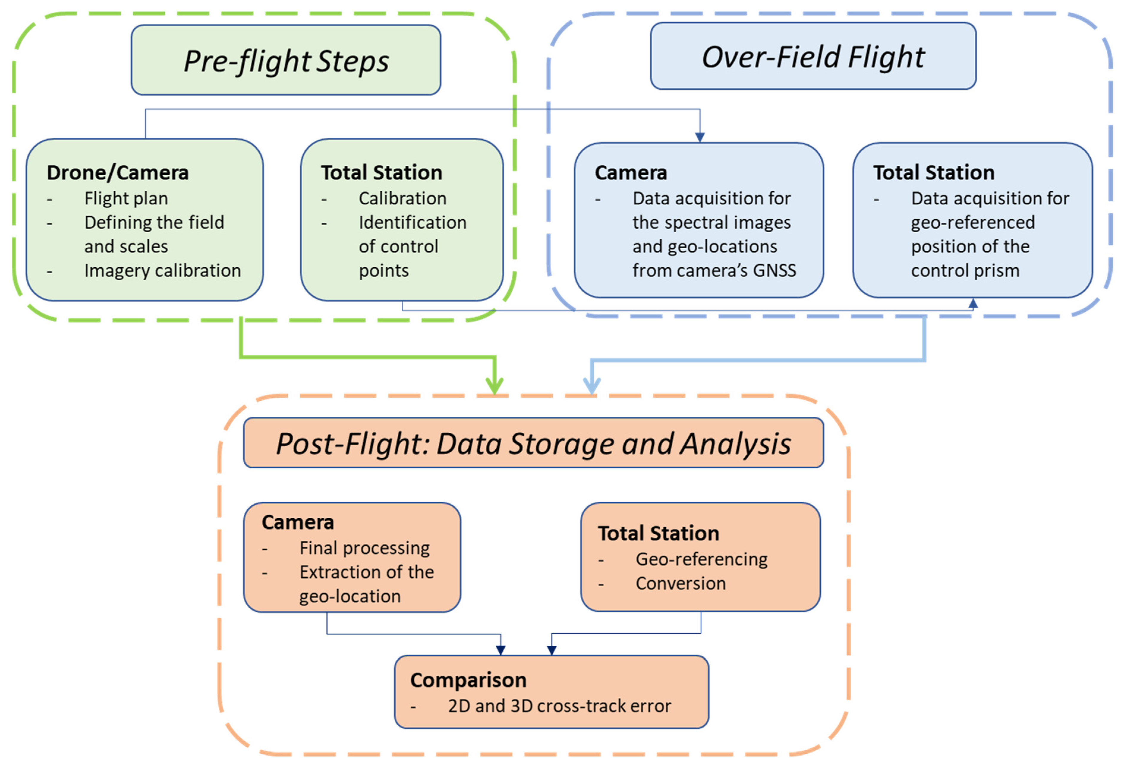
2.1. Workflow

The workflow that describes the steps followed during the pre-flight, over-field flight, and after the flight, in terms of the instrumentation and setup, data acquisition, and data analysis, respectively, is given in Figure 1. In the initial phase, it is very important to properly plan the flight since the flight path, adequate overlap for both longitudinal and transverse, and sunlight angle have a significant impact on the radiometric calibration of the multispectral camera. Besides that, the identification of control points in the field was one of the initial, but very crucial for the accurate performance of the TS. This was followed by the data acquisition for both spectral images and the georeferenced position of the attached prism, in terms of data from the multispectral camera and the TS, respectively. The final phase included the analysis and comparison of both camera and TS data. All three phases are described in detail in the following sections.

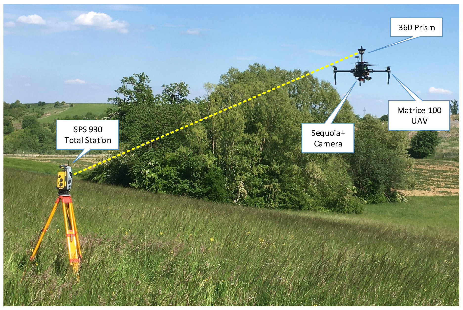
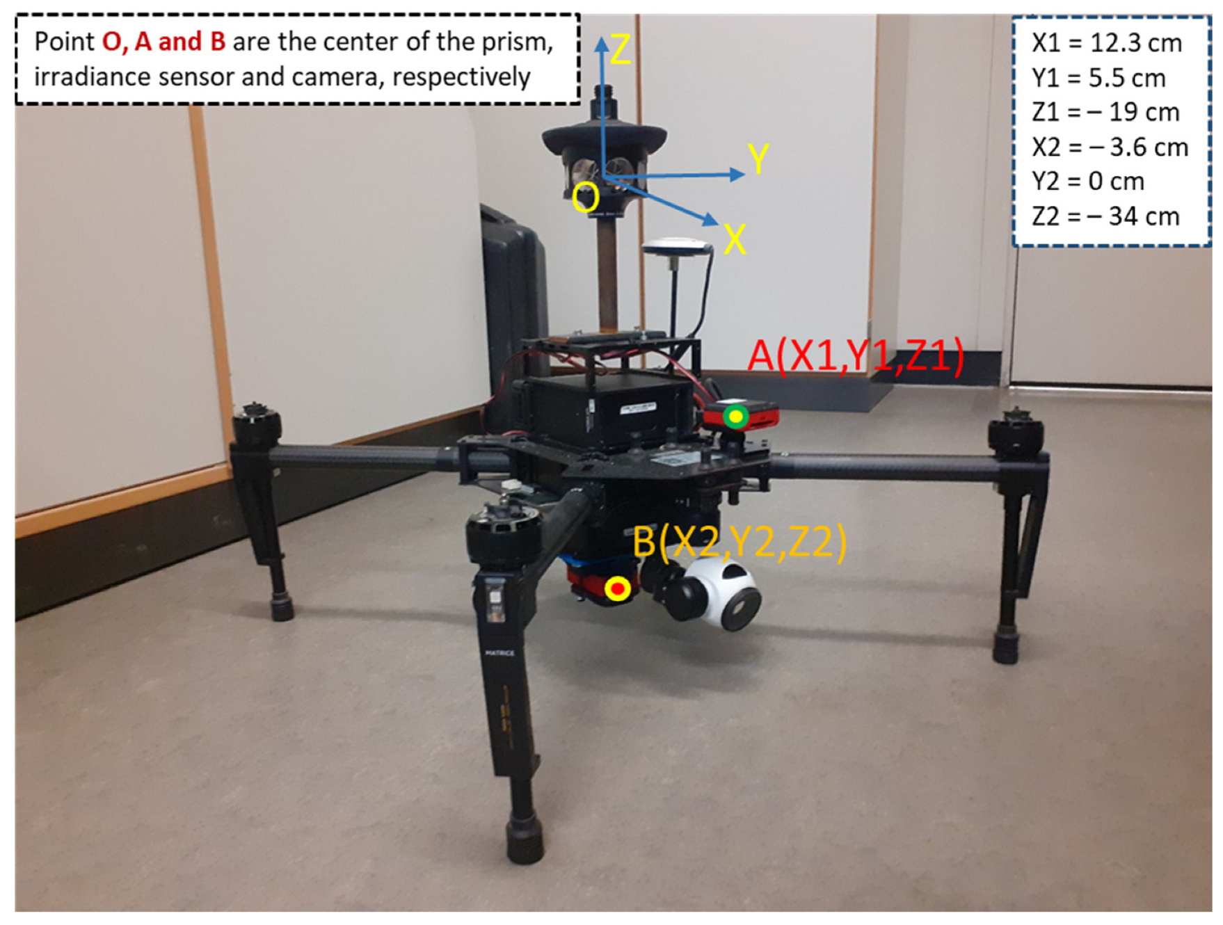
2.2. Instrumentation

The utilized instrumentation is presented in Figure 2. A Sequoia+ multispectral camera was mounted on a Matrice 100 UAV (DJI, Nanshan, Shenzhen, China). To assess the position accuracy of the camera, an SPS930 universal TS (Trimble, Sunnyvale, CA, USA) was used to track a Trimble 360 prism also mounted on the UAV. The main technical characteristics of the camera are presented in

Table 1. Sequoia+ multispectral camera technical data.

Parameter	Value
Weight	135 g (4.8 oz), including sunshine sensor and cable
Sensor spectral characteristics	Green Band 1: 550 nm, 40 nm bandwidth Red Band 2: 660 nm, 40 nm bandwidth Red-edge Band 3: 735 nm, 10 nm bandwidth Near-infrared Band 4: 790 nm, 40 nm bandwidth
Focal Length	3.98 mm
35 mm equivalent focal length	30 mm
Imager resolution	1280 horizontal × 960 vertical pixels (1.22 megapixels)
Image size	4.8 mm × 3.6 mm
Physical Pixel Size	0.00375 × 0.00375 mm
Radiometric resolution	10-bit sensor (1024 BVs) stored as 16-bit (65,536 BVs)

, while the technical characteristics of the SPS930 TS can be found in

Table 2. SPS 930 TS technical data.

Parameter	Value
Distance measurement accuracy	±(4 mm + 2 ppm)
Angle measurement horizontal and vertical accuracy	0.3 mgon
Measurement range	2500 m
Data output rate	max 20 Hz
Maximum radial speed of target	114° s−1
Maximum axial speed of target	6 m s−1
Synchronized measurement data	<1 ms

. The assessing device needs to have at least four times higher accuracy (4:1 test accuracy ratio (TAR)) compared to the assessed device for the results to be reliable [22], while usually a TAR of 10:1 is preferable.

In Figure 3, a more detailed illustration of the used Matrice 100 UAV together with the Sequoia+ multispectral camera is presented. To obtain multispectral imagery from the examined vegetation, the camera is usually mounted at the bottom part of the UAV facing downwards. However, the GNSS receiver of the camera is located in the sunshine sensor, which is mounted on the main plate to be able to have a line of sight with the satellites in orbit and also measure the sunshine for calibration purposes. This aspect (i.e., having the camera and the receiver at different positions) is already introducing a fixed offset between these two components and the recommendation is to place them as close as possible. However, this offset is not the focus of the present study, which examines the position accuracy of the GNSS receiver under service conditions. Whenever the camera position is mentioned in the paper, it is referring to the GNSS receiver, which is assigning the position information to the obtained images. The GNSS receiver could receive a differential signal (D-GNSS) from the EGNOS (European geostationary navigation overlay service) SBAS (satellite-based augmentation systems).

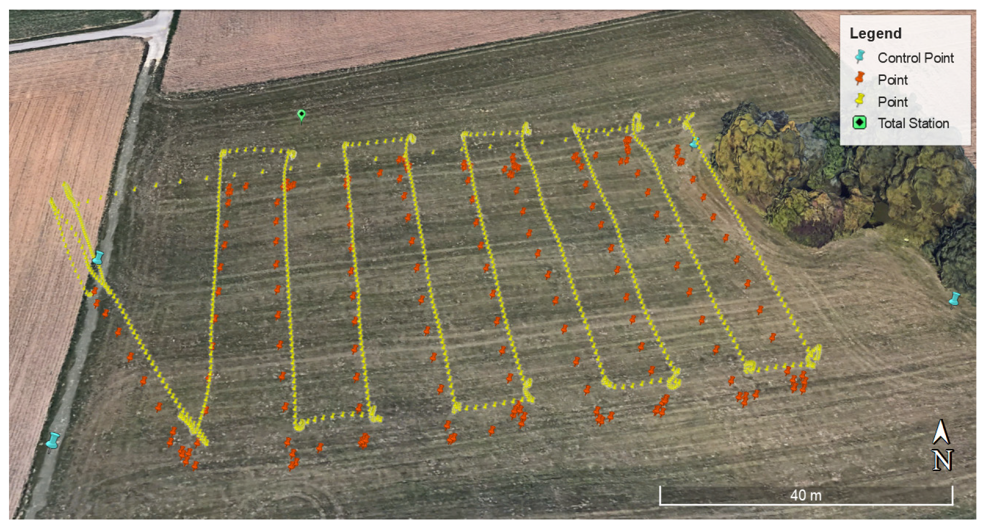
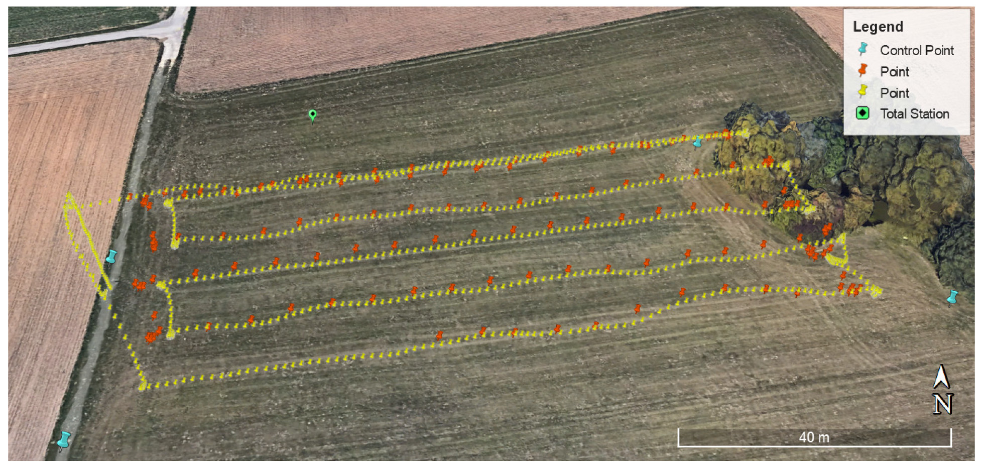
2.3. Experimental Design and Data Acquisition

The experiments took place at the research station of the University of Hohenheim (48°44′39.6″ N 8°55′25.9″ E-Ihinger Hof, Renningen, Germany). For comparison reasons, two sets of measurements were obtained. In the first set, the route of the UAV was designed to follow parallel passes along the East–West (E–W) axis, while in the second one, the UAV was moving along the South–North (S–N) axis. The satellite view with the positions of the prism (yellow pins) and the positions of the images (red pins) for the E–W and S–N experiment is presented in Figure 4 and Figure 5, respectively. As it can be seen from the two figures, a deviation occurred from the corresponding axes, but this was inevitable due to the orientation of the field that was used for setting up the performed routes, and it was regarded as acceptable for this research.

The Trimble SCS900 Site Controller software, running on a Trimble Yuma 2 tablet computer, was used to acquire and store data from the TS. The 3D position data were transmitted from the TS as long as the current measurement varied at least 1 mm from the previous one but with a maximum frequency of 3 Hz. Although there are available prisms for the specific TS that can reach up to 20 Hz and have been used by the authors in previous research [23,24], the utilized 360 prism was chosen due to its reduced weight (0.39 kg).

Initially, a stationing procedure for the TS was necessary. This is a method of determining the location of one unknown point in relation to known points. In this case, the unknown point was the point of the TS. To do this, several stationing points (i.e., points with known coordinates) are necessary. Four points were marked on the field surface (Figure 4 and Figure 5) and the position of these points was measured by using an RTK-GNSS. After the coordinates of these points are inserted in the TS and are also measured by placing the prism on the fixed locations, the TS performs internally a geometric rigid transformation to be able to output the position data in a fixed coordinate system. The world geodetic system 84 (WGS84) was chosen as the reference geodetic datum as this was also used by the D-GNSS receiver.

To have a direct comparison in meters, the TS was configured to output the position data in the Universal Transverse Mercator (UTM) coordinate system. Thus, the obtained position data contained the values of easting, northing, and elevation (orthometric height) in m. The D-GNSS receiver of the camera was outputting the position in latitude, longitude, altitude, and ellipsoid height. To make the comparison possible, first, the geoid height, which was equal to 48.681 m for the location of the experiments, was subtracted from the TS elevation measurements to get the ellipsoid height as the D-GNSS measurements. Second, the latitude and longitude data of the camera were converted to UTM coordinates.

The multispectral camera was obtaining five images every one second (1 Hz) based on a GeoTIFF format. Of the five images, one was the RGB (red-green-blue) and the rest four were from the bands that are presented in Table 1 (i.e., green, red, red-edge, and near-infrared). Georeferencing information was embedded within the TIFF files by using position data from the D-GNSS receiver. These files were imported into MATLAB (Mathworks, Natick, MA, USA) for further analysis.

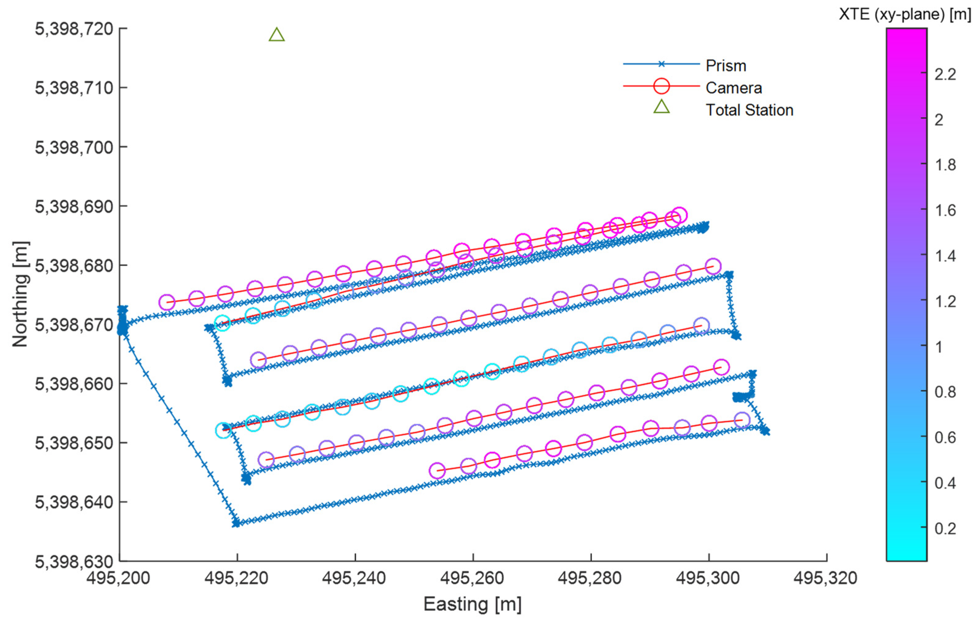
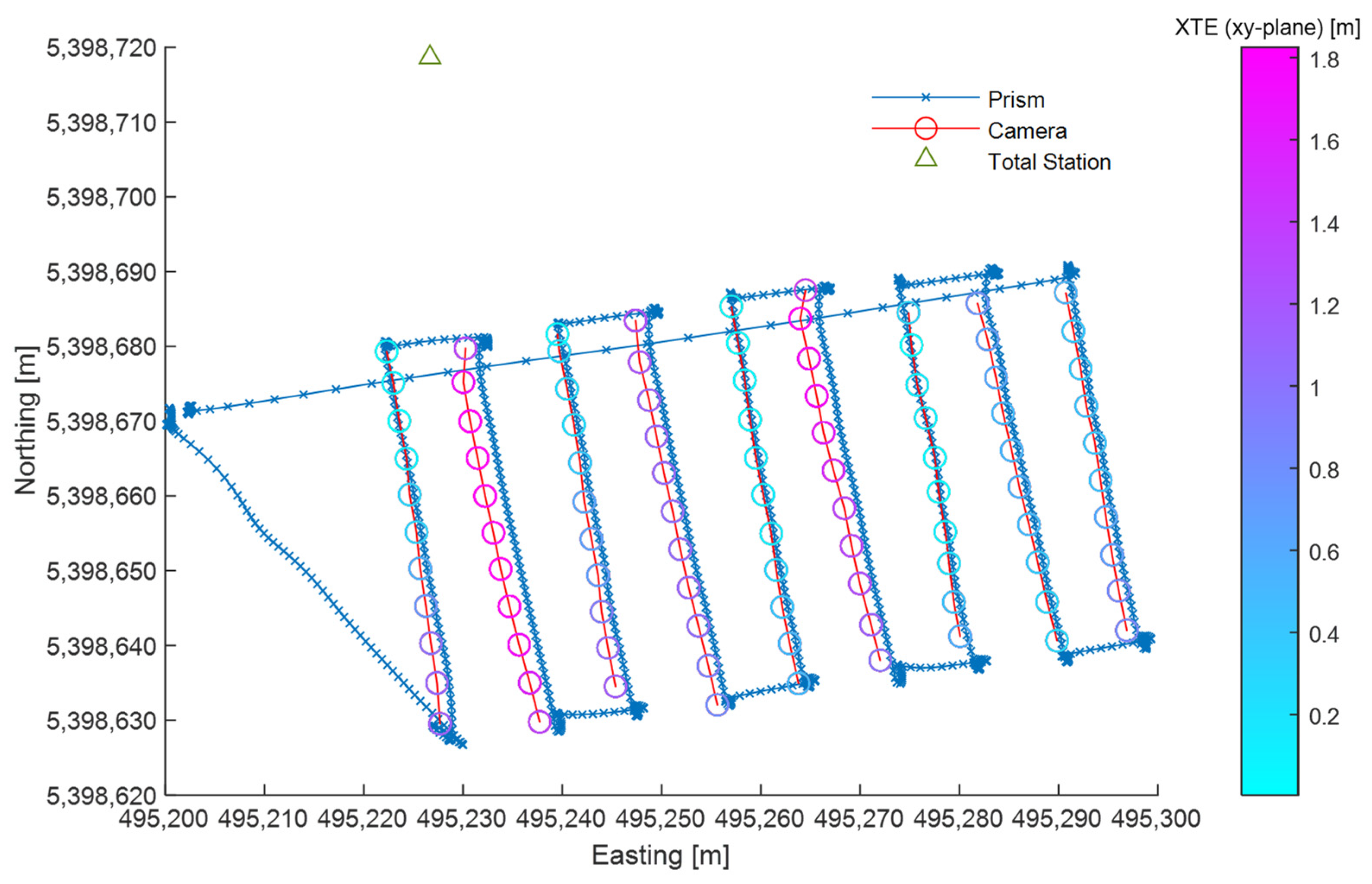
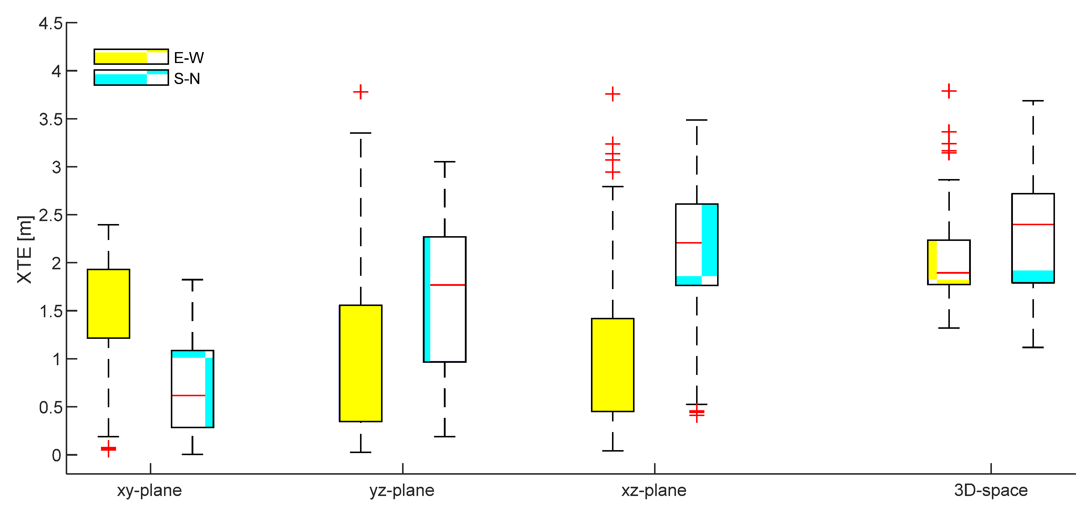
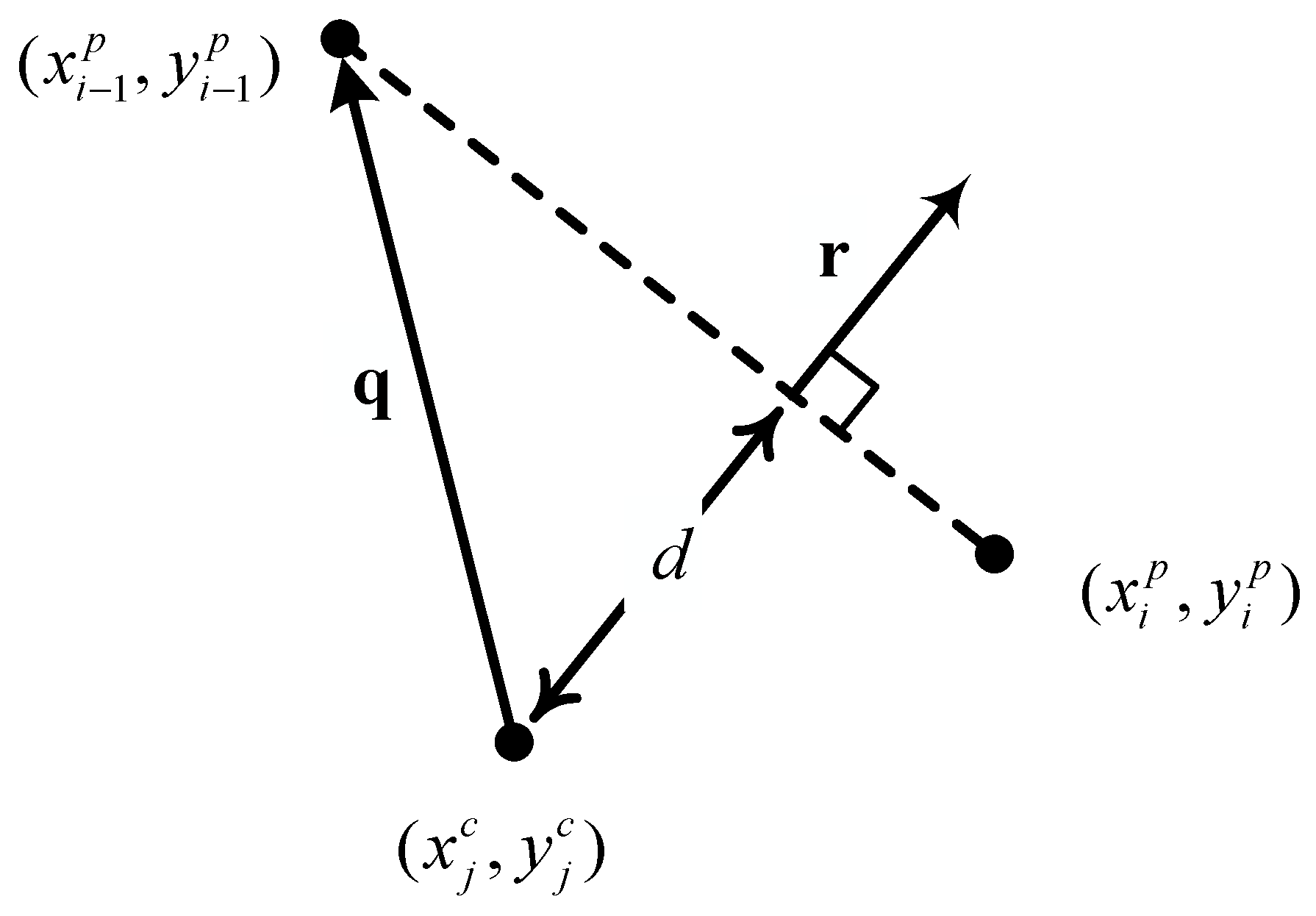
2.4. 2D Cross-Track Error

As a first accuracy assessment criterion for the camera position data, the 2D cross-track error (XTE) was chosen. The geometrical representation of the XTE is presented in Figure 6. The XTE is the horizontal distance $d$ between any measured position of the camera $p_j^c=\left(x_j^c,y_j^c\right)$ $\left(j=1,\dots ,m\right)$ and the specific path of the prism $p_i^p=\left(x_i^p,y_i^p\right)$ $\left(i=1,\dots ,n\right)$, where $m$ and $n$ represent the total number of measured points for the camera and the prism, respectively.

The vector that is perpendicular to the line connecting the two reference points $p_{i-1}^p$ and $p_i^p$, is calculated by

$$r=\left[\begin{array}{c}{y}_i^p-y_{i-1}^p\\ -\left(x_i^p-x_{i-1}^p\right)\end{array}\right]$$

Consider $q$ a vector from the camera $p_j^c$ to the first prism point $p_{i-1}^p$ defined by

$$q=\left[\begin{array}{c}{x}_{i-1}^p-x_j^c\\ y_{i-1}^p-y_j^c\end{array}\right],$$

then the XTE is equal to the distance $d$, which is given by projecting $q$ onto $r$ provided by

$$d=\left|{\mathrm{proj}}_{\mathrm{r}}q\right|=\left|\widehat{r}·q\right|=\frac{\left|r·q\right|}{\left|r\right|}=\frac{\left|\left(x_i^p-x_{i-1}^p\right)\left(y_{i-1}^p-y_j^c\right)-\left(x_{i-1}^p-x_j^c\right)\left(y_i^p-y_{i-1}^p\right)\right|}{\sqrt{{\left(x_i^p-x_{i-1}^p\right)}^2+{\left(y_i^p-y_{i-1}^p\right)}^2}}$$

(1)

where $\widehat{r}$ is the unit vector in the direction of $r$.

To find the 2D XTE for all measured position data, an algorithm was developed that was calculating the distance to all points of the prism for each measured camera point $p_j^c$. Subsequently, the two prism points with the smallest distance to $p_j^c$ were chosen as $p_{i-1}^p$ and $p_i^p$, to find the XTE by solving Equation (1). To find the horizontal 2D XTE in the $xy$-plane, the procedure was as described above by using the easting and northing position data. In addition to the $xy$-plane, the 2D XTE was calculated for the $yz$- and the $xz$-plane by following the same procedure, but by replacing in each case the corresponding axis, i.e., for the $yz$-plane the easting and elevation was used while the XTE in the $xz$-plane was calculated based on the northing and elevation data.

From the resulted XTEs the fixed 2D Euclidean distance between points P and C (points O and A in Figure 3, respectively) was subtracted based on the following:

$$xy-\mathrm{plane}: d_{P{C}_{xy}}=\sqrt{{\left(x^p-x^c\right)}^2+{\left(y^p-y^c\right)}^2}=0.1347 \mathrm{m}$$

(2)

$$yz-\mathrm{plane}: d_{P{C}_{yz}}=\sqrt{{\left(y^p-y^c\right)}^2+{\left(z^p-z^c\right)}^2}=0.1978 \mathrm{m}$$

(3)

$$xz-\mathrm{plane}: d_{P{C}_{xz}}=\sqrt{{\left(x^p-x^c\right)}^2+{\left(z^p-z^c\right)}^2}=0.2263 \mathrm{m}$$

(4)

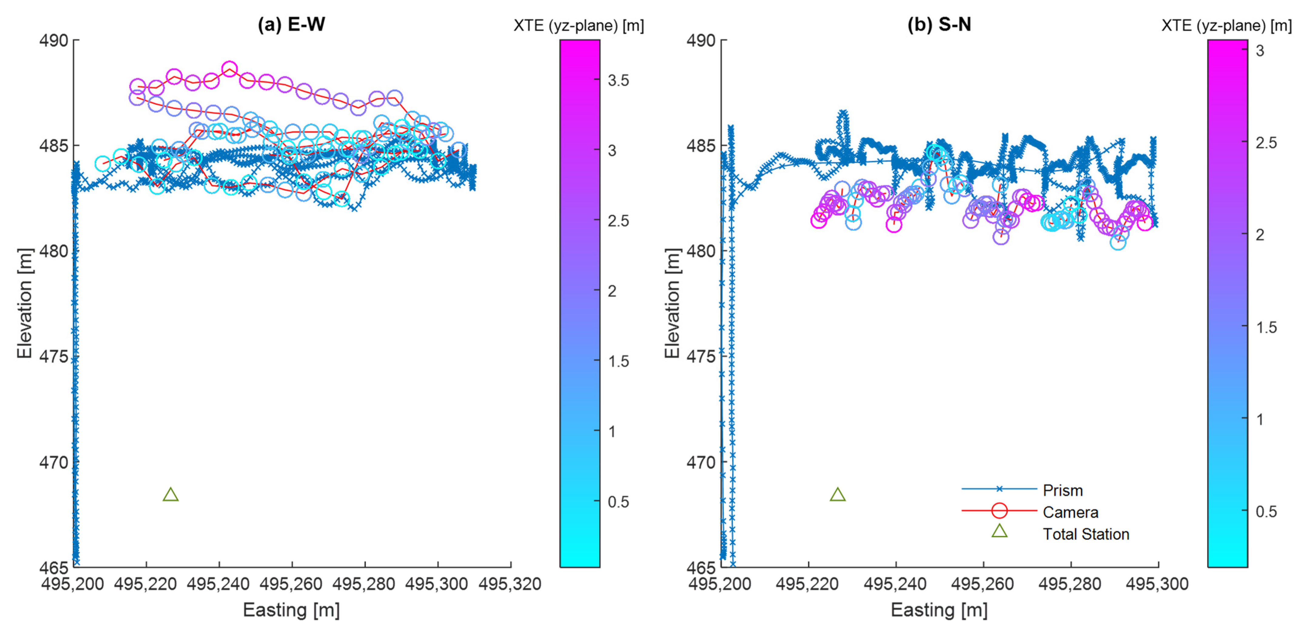
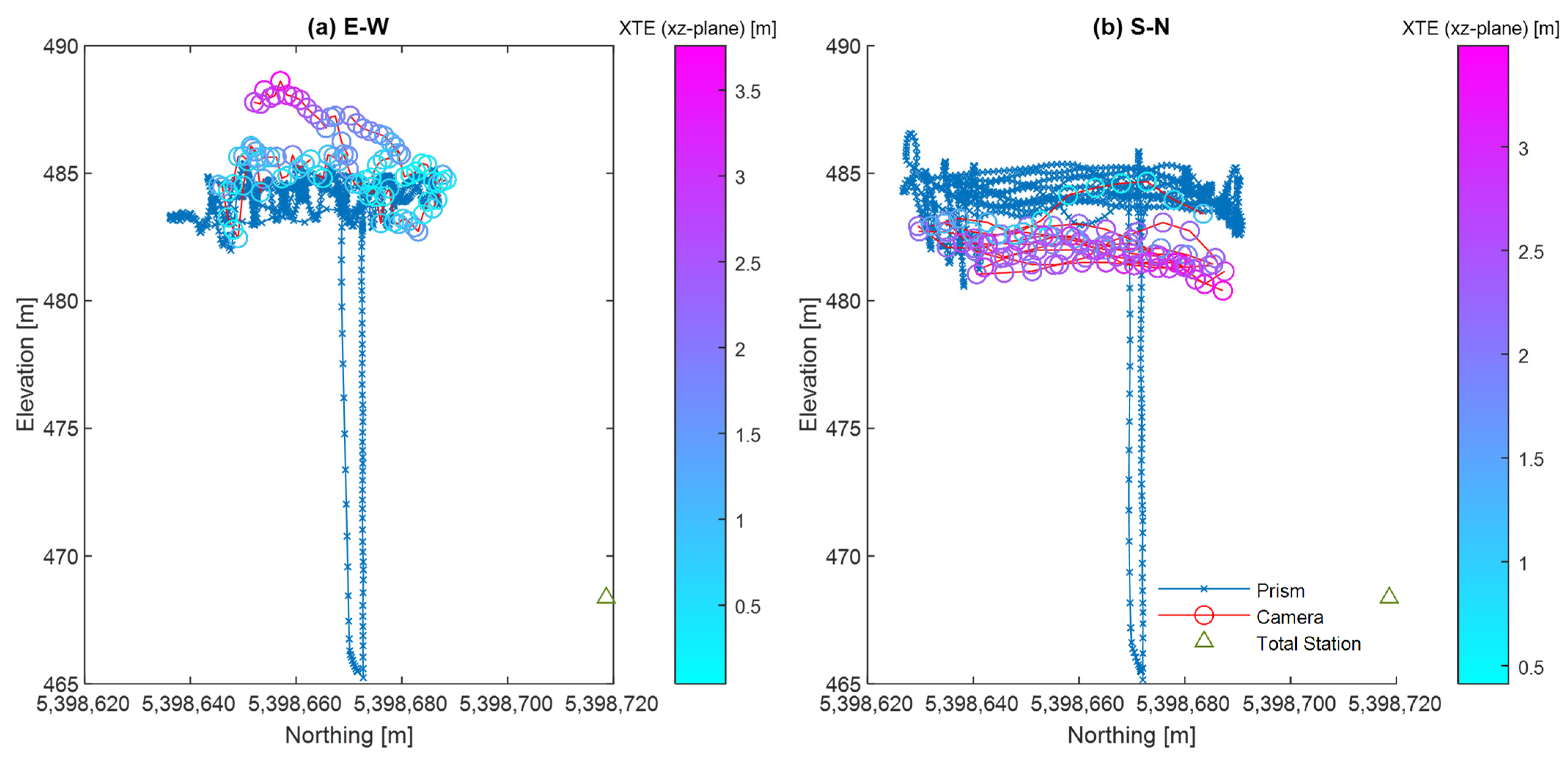
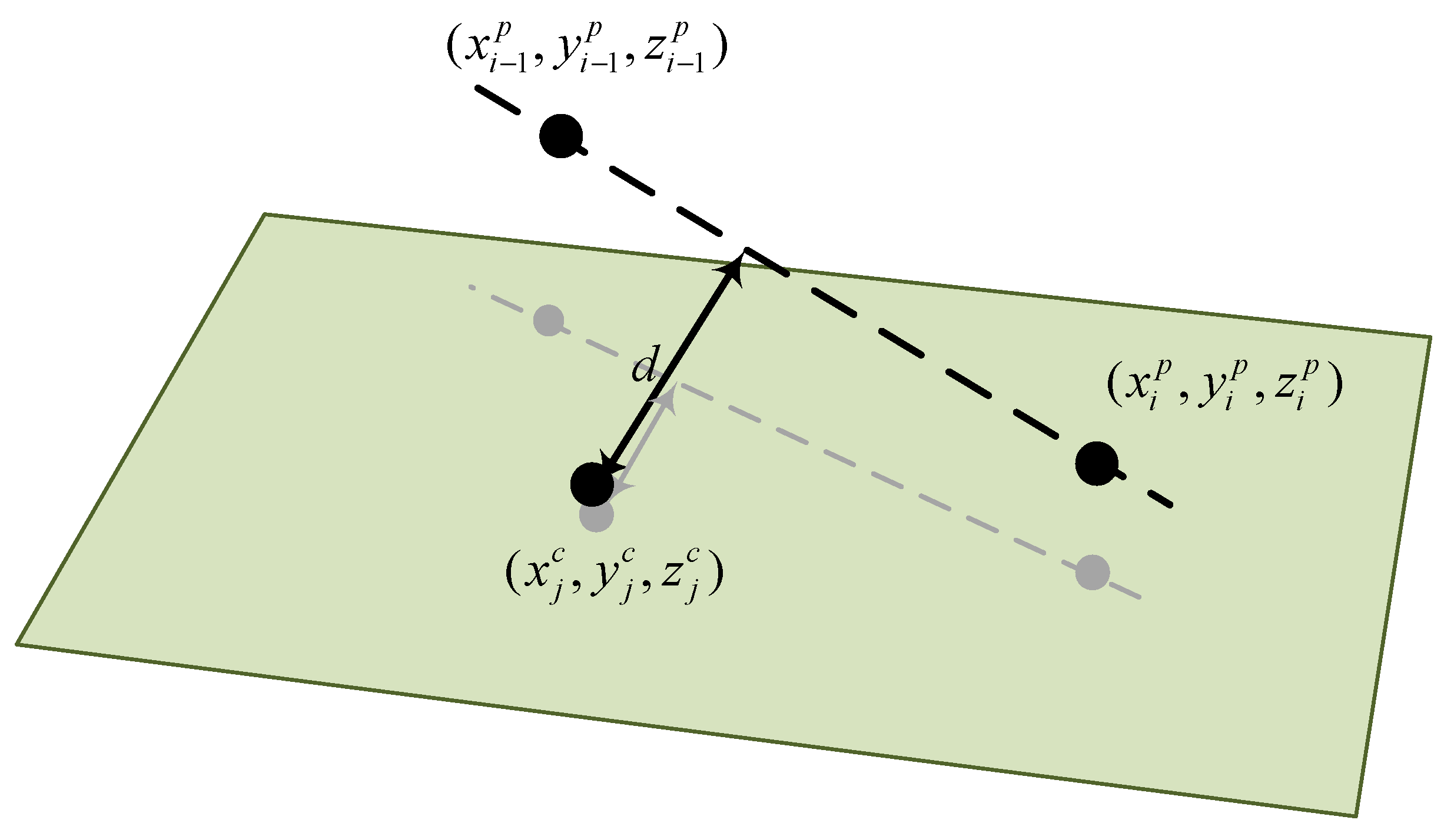
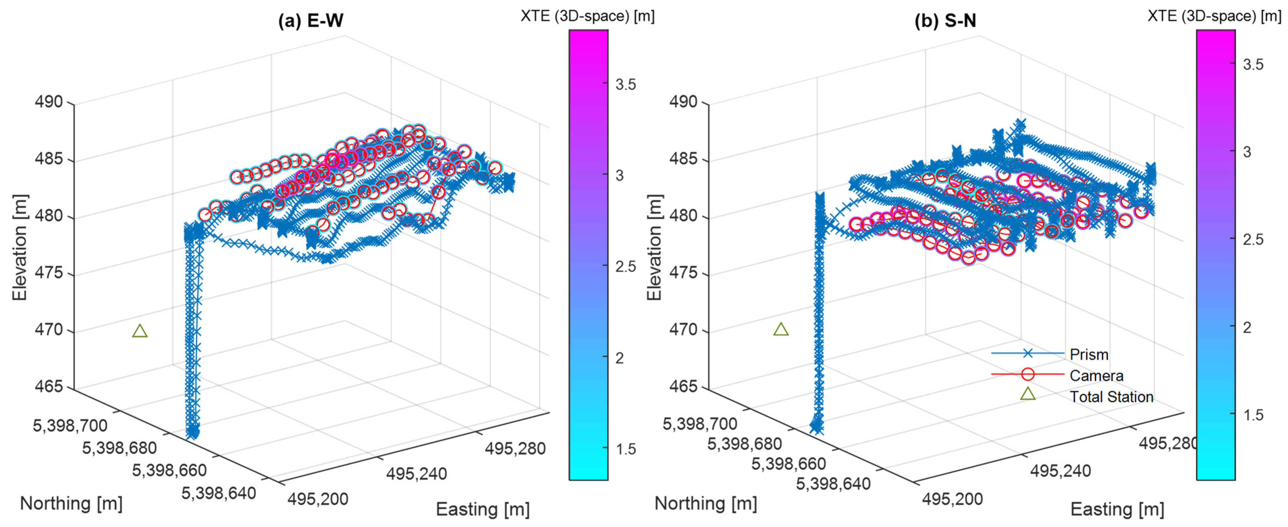
2.5. 3D Cross-Track Error

The next assessment criterion was the 3D XTE to define the distance between any camera position $p_j^c=\left(x_j^c,y_j^c,z_j^c\right)$ $\left(j=1,\dots ,m\right)$ and the line segment defined by two consecutive prism points $p_{i-1}^p=\left(x_{i-1}^p,y_{i-1}^p,z_{i-1}^p\right)$ and $p_i^p=\left(x_i^p,y_i^p,z_i^p\right)$. The geometrical representation of the 3D XTE is presented in Figure 7 and is given by the following equation [25]

$$d=\frac{\left|\left(p_j^c-p_{i-1}^p\right)\times \left(p_j^c-p_i^p\right)\right|}{\left|\left(p_i^p-p_{i-1}^p\right)\right|}$$

(5)

where $\times$ denotes the cross product. It should be noted that Equation (5) is equivalent to Equation (1) with all vectors having zero z-components. From the resulted XTE the 3D Euclidean distance between points P and C (points O and A in Figure 3 respectively) was subtracted. This distance was equal to:

$$d_{PC\_3D}=\sqrt{\left({\left(x^p-x^c\right)}^2+{\left(y^p-y^c\right)}^2+{\left(z^p-z^c\right)}^2\right)}=0.2329 \mathrm{m}$$

(6)

3. Results and Discussion

3.1. 2D Cross-Track Error

In Figure 8, the obtained position data from the camera (circles) and the prism (stars) of the E–W experiment in the $xy$-plane are presented. These position data refer to points O and A, as shown in Figure 3. Since only the images that are acquired during the parallel passes of the UAV are usually utilized in agriculture-related operations, the images that corresponded to the turning parts of the route were filtered out. The color of the circles corresponds to the 2D XTE calculated by using Equation (1) and by subtracting the fixed distance of Equation (2). As it can be seen from the colorbar on the right side of the figure, the XTE reached a value almost equal to 2.4 m. The same information for the S–N experiment is presented in Figure 9. In that case, the XTE had a maximum value of around 1.8 m. It is already clear from Figure 8 and Figure 9 that the XTE is not a value that varies rapidly while it indicates a drift. This has been identified by the authors in previous research where the position assessment offered by a D-GNSS was also examined [26].

In Figure 10, the camera and the prism positions of the E–W (Figure 10a) and the S–N (Figure 10b) experiment in the $yz$-plane can be seen. The same information in the $xz$-plane is presented in Figure 11a,b, respectively. An XTE that reaches up to more than 3.5 for both planes for the E–W experiment can be seen, while for the S–N experiment, the XTE lies between 3 and 3.5 m. For the E–W experiment, several camera position data are above the prism position. For the S–N experiment, the opposite can be seen as several camera position data are indicated below the prism position. In any case, the XTE in the vertical planes appears to be higher than in the horizontal plane.

In Figure 12 the camera and the prism position data of the E–W (Figure 12a) and the S–N (Figure 12b) experiment in the 3D space can be seen. The Euclidean distance between the center of the prism and the center of the irradiance sensor, where the GNSS receiver of the camera was located, was subtracted from the results.

3.2. Accuracy Assessment

The XTE box plots for all obtained data were produced using MATLAB’s function boxplot, and are presented in Figure 13. On each box, the central red line mark is the median, and the edges of the box are the 25th and 75th percentiles. The distance between the bottom and top of each box is the interquartile range. The whisker extends to the most extreme data value that is not an outlier (a value that is more than 1.5 times the interquartile range away from the bottom or top of the box), while the outliers are illustrated with a red cross. It can be seen that the XTE for the E–W experiment had a higher median in the $xy$-plane compared to the $yz$- and $xz$-plane. For the S–N experiment, this was exactly the opposite with a lower XTE median value for the $xy$-plane. As it is depicted, although it is important to know which plane the XTE come from, it is essential to calculate the 3D XTE to get a clearer view of the results. This becomes evident in the right side of Figure 13 where the 3D XTE appears to be in a similar range for both E–W and S–N experiments.

To get a better insight into the resulted XTE, the summary statistics for all performed experiments are presented in

Table 3. Summary statistics for all experiments performed.

		XTE [m]
		Mean	St. Dev.	95th per.	Max
$xy$-plane	E–W	1.47	0.65	2.33	2.39
	S–N	0.74	0.55	1.78	1.82
$yz$-plane	E–W	1.08	0.89	3.17	3.78
	S–N	1.67	0.74	2.80	3.05
$xz$-plane	E–W	1.05	0.85	2.94	3.76
	S–N	2.12	0.68	3.01	3.49
3D-space	E–W	2.05	0.45	3.14	3.79
	S–N	2.35	0.63	3.34	3.69

. As it was already evident from the boxplots, the mean 2D XTE value in the $xy$-plane for the E–W experiment was almost double compared to the S–N experiment (1.47 m for E–W and 0.74 m for S–N). The opposite was for the $yz$- and $xz$-plane where the mean 2D XTE in the S–N experiment were higher compared to the XTE in the E–W experiments.

However, the mean 3D XTE was 0.3 m lower for the E–W compared to the S–N (2.05 to 2.35 m, respectively). The same applies to the 95th percentile where the 3D XTE in E–W was 0.2 m lower compared to the S–N (3.14 m compared to 3.34 m). When comparing the maximum 3D XTE values for both experiments, a slight difference of 0.1 resulted (3.79 to 3.69 m). In general, the resulted 3D XTE is in accordance with the work of other researchers that are reporting 2.0 to 2.5 m of accuracy for the specific GNSS receiver [27].

An important aspect that can be seen from the results is that the position error in the vertical dimension ($yz$- and $xz$-planes) is higher than the error in the horizontal $xy$-plane and should always be assessed and not be neglected when using the camera-obtained information for agronomic applications.

4. Conclusions

As UAV-mounted multispectral cameras are very promising in obtaining information related to site-specific applications, the accuracy of these devices is expected to be a topic of increasing interest. A methodology was presented on how this could be achieved by utilizing a TS. From the results, it can be seen that a D-GNSS receiver can offer imagery with a 3D position accuracy of up to 3.79 m. Commercial software that is analyzing the obtained images can improve this accuracy. However, when researchers are developing their algorithms, error filtering can be a difficult task and possible error sources should be reduced as much as possible as the translation of this information from the camera position to the area of interest, which is usually the field surface, can increase this position error.

Future work should include obtaining data from an IMU mounted on the UAV to be able to correct the position error of the camera images. Furthermore, concurrent measurements should be considered as this is an important factor in finding the along-the-track error but also correcting the images in post-processing. Site-specific farming activities such as variable-rate fertilization and spraying could significantly benefit from eliminating the position error by using the introduced methodology. This will result in a higher accuracy of the developed prescription maps and, consequently, increased accuracy of the as-applied rates as well as optimized machine performance.

References

1. Franzini, M.; Ronchetti, G.; Sona, G.; Casella, V. Geometric and Radiometric Consistency of Parrot Sequoia Multispectral Imagery for Precision Agriculture Applications. Appl. Sci. 2019, 9, 5314. [Google Scholar] [CrossRef] [Green Version]
2. Daponte, P.; De Vito, L.; Glielmo, L.; Iannelli, L.; Liuzza, D.; Picariello, F.; Silano, G. A Review on the Use of Drones for Precision Agriculture. IOP Conf. Ser. Earth Environ. Sci. 2019, 275, 012022. [Google Scholar] [CrossRef]
3. Sanz-Ablanedo, E.; Chandler, J.H.; Rodríguez-Pérez, J.R.; Ordóñez, C. Accuracy of Unmanned Aerial Vehicle (UAV) and SfM Photogrammetry Survey as a Function of the Number and Location of Ground Control Points Used. Remote Sens. 2018, 10, 1606. [Google Scholar] [CrossRef] [Green Version]
4. Islam, N.; Rashid, M.M.; Pasandideh, F.; Ray, B.; Moore, S.; Kadel, R. A Review of Applications and Communication Technologies for Internet of Things (Iot) and Unmanned Aerial Vehicle (Uav) Based Sustainable Smart Farming. Sustainability 2021, 13, 1821. [Google Scholar] [CrossRef]
5. Boursianis, A.D.; Papadopoulou, M.S.; Diamantoulakis, P.; Liopa-Tsakalidi, A.; Barouchas, P.; Salahas, G.; Karagiannidis, G.; Wan, S.; Goudos, S.K. Internet of Things (IoT) and Agricultural Unmanned Aerial Vehicles (UAVs) in Smart Farming: A Comprehensive Review. Internet Things 2022, 18, 100187. [Google Scholar] [CrossRef]
6. Almalki, F.A.; Soufiene, B.O.; Alsamhi, S.H.; Sakli, H. A Low-Cost Platform for Environmental Smart Farming Monitoring System Based on Iot and UAVs. Sustainability 2021, 13, 5908. [Google Scholar] [CrossRef]
7. Buters, T.M.; Belton, D.; Cross, A.T. Multi-Sensor Uav Tracking of Individual Seedlings and Seedling Communities at Millimetre Accuracy. Drones 2019, 3, 81. [Google Scholar] [CrossRef] [Green Version]
8. Zaman-Allah, M.; Vergara, O.; Araus, J.L.; Tarekegne, A.; Magorokosho, C.; Zarco-Tejada, P.J.; Hornero, A.; Albà, A.H.; Das, B.; Craufurd, P.; et al. Unmanned Aerial Platform-Based Multi-Spectral Imaging for Field Phenotyping of Maize. Plant. Methods 2015, 11, 1–10. [Google Scholar] [CrossRef] [PubMed] [Green Version]
9. Yue, J.; Lei, T.; Li, C.; Zhu, J. The Application of Unmanned Aerial Vehicle Remote Sensing in Quickly Monitoring Crop Pests. Intell. Autom. Soft Comput. 2012, 18, 1043–1052. [Google Scholar] [CrossRef]
10. Zarco-Tejada, P.J.; Guillén-Climent, M.L.; Hernández-Clemente, R.; Catalina, A.; González, M.R.; Martín, P. Estimating Leaf Carotenoid Content in Vineyards Using High Resolution Hyperspectral Imagery Acquired from an Unmanned Aerial Vehicle (UAV). Agric. For. Meteorol. 2013, 171–172, 281–294. [Google Scholar] [CrossRef] [Green Version]
11. Chen, S.; McGovern, E.; Gilmer, A. Coastal Dune Vegetation Mapping Using a Multispectral Sensor Mounted on an UAS. Remote Sens. 2019, 11, 1814. [Google Scholar] [CrossRef] [Green Version]
12. Mesas-Carrascosa, F.J.; Torres-Sánchez, J.; Clavero-Rumbao, I.; García-Ferrer, A.; Peña, J.M.; Borra-Serrano, I.; López-Granados, F. Assessing Optimal Flight Parameters for Generating Accurate Multispectral Orthomosaicks by Uav to Support Site-Specific Crop Management. Remote Sens. 2015, 7, 12793–12814. [Google Scholar] [CrossRef] [Green Version]
13. Shahbazi, M.; Sohn, G.; Théau, J.; Menard, P. Development and Evaluation of a UAV-Photogrammetry System for Precise 3D Environmental Modeling. Sensors 2015, 15, 27493–27524. [Google Scholar] [CrossRef] [Green Version]
14. Turner, D.; Lucieer, A.; Watson, C. An Automated Technique for Generating Georectified Mosaics from Ultra-High Resolution Unmanned Aerial Vehicle (UAV) Imagery, Based on Structure from Motion (SFM) Point Clouds. Remote Sens. 2012, 4, 1392–1410. [Google Scholar] [CrossRef] [Green Version]
15. Hugenholtz, C.; Brown, O.; Walker, J.; Barchyn, T.; Nesbit, P.; Kucharczyk, M.; Myshak, S. Spatial Accuracy of UAV-Derived Orthoimagery and Topography: Comparing Photogrammetric Models Processed with Direct Geo-Referencing and Ground Control Points. GEOMATICA 2016, 70, 21–30. [Google Scholar] [CrossRef]
16. Mian, O.; Lutes, J.; Lipa, G.; Hutton, J.J.; Gavelle, E.; Borghini, S. Accuracy Assessment of Direct Georeferencing for Photogrammetric Applications on Small Unmanned Aerial Platforms. Int. Arch. Photogramm. Remote Sens. Spat. Inf. Sci.-ISPRS Arch. 2016, 40, 77–83. [Google Scholar] [CrossRef] [Green Version]
17. Pix4D Mapper 4.1 User Manual. Available online: support.pix4d.com/hc/en-us/sections/360003718992-Manual (accessed on 18 April 2022).
18. Di Gennaro, S.F.; Toscano, P.; Gatti, M.; Poni, S.; Berton, A.; Matese, A. Spectral Comparison of UAV-Based Hyper and Multispectral Cameras for Precision Viticulture. Remote Sens. 2022, 14, 449. [Google Scholar] [CrossRef]
19. Assmann, J.J.; Kerby, J.T.; Cunliffe, A.M.; Myers-Smith, I.H. Vegetation Monitoring Using Multispectral Sensors—Best Practices and Lessons Learned from High Latitudes. J. Unmanned Veh. Syst. 2019, 7, 54–75. [Google Scholar] [CrossRef] [Green Version]
20. Olsson, P.O.; Vivekar, A.; Adler, K.; Garcia Millan, V.E.; Koc, A.; Alamrani, M.; Eklundh, L. Radiometric Correction of Multispectral Uas Images: Evaluating the Accuracy of the Parrot Sequoia Camera and Sunshine Sensor. Remote Sens. 2021, 13, 577. [Google Scholar] [CrossRef]
21. Paraforos, D.S.; Reutemann, M.; Sharipov, G.; Werner, R.; Griepentrog, H.W. Total Station Data Assessment Using an Industrial Robotic Arm for Dynamic 3D In-Field Positioning with Sub-Centimetre Accuracy. Comput. Electron. Agric. 2017, 136, 166–175. [Google Scholar] [CrossRef]
22. Caldwell, D. ANSI/NCSL Z540.3:2006: Requirements for the Calibration of Measuring and Test Equipment. NCSLI Meas. 2006, 1, 26–30. [Google Scholar] [CrossRef]
23. Sharipov, G.M.; Heiß, A.; Eshkabilov, S.L.; Griepentrog, H.W.; Paraforos, D.S. Variable Rate Application Accuracy of a Centrifugal Disc Spreader Using ISO 11783 Communication Data and Granule Motion Modeling. Comput. Electron. Agric. 2021, 182, 106006. [Google Scholar] [CrossRef]
24. Sharipov, G.M.; Paraforos, D.S.; Griepentrog, H.W. Implementation of a Magnetorheological Damper on a No-till Seeding Assembly for Optimising Seeding Depth. Comput. Electron. Agric. 2018, 150, 465–475. [Google Scholar] [CrossRef]
25. Weisstein, E.W. Point-Line Distance—3-Dimensional. From MathWorld—A Wolfram Web Resource. Available online: https://mathworld.wolfram.com/Point-LineDistance3-Dimensional.html (accessed on 18 April 2022).
26. Heiß, A.; Paraforos, D.S.; Griepentrog, H.W. Determination of Cultivated Area, Field Boundary and Overlapping for A Plowing Operation Using ISO 11783 Communication and D-GNSS Position Data. Agriculture 2019, 9, 38. [Google Scholar] [CrossRef] [Green Version]
27. Kikutis, R.; Stankūnas, J.; Rudinskas, D.; Masiulionis, T. Adaptation of Dubins Paths for UAV Ground Obstacle Avoidance When Using a Low Cost On-Board GNSS Sensor. Sensors 2017, 17, 2223. [Google Scholar] [CrossRef]
Figure 1. The workflow for the experimental setup, data acquisition from the employed sensors, and data analysis, as well as the comparison for defining the cross-track errors.
Agriculture 12 00885 g001
Figure 2. The utilized SPS 930 total station tracking a 360 prism on the Matrice 100 UAV, which was also carrying a Sequoia+ multispectral camera.
Agriculture 12 00885 g002
Figure 3. The utilized Matrice 100 UAV and the mounted Sequoia+ multispectral camera.
Agriculture 12 00885 g003
Figure 4. Satellite view with the positions of the prism (yellow pins) and the positions of the images (red pins). The direction of movement was as close as possible along the East–West axis (E–W). The TS and the four control points that were used for the stationing are also indicated (Landsat / Copernicus, Google Earth, edited).
Agriculture 12 00885 g004
Figure 5. Satellite view with the positions of the prism (yellow pins) and the positions of the images (red pins). The direction of movement was as close as possible along the South–North axis (S–N). The TS and the four control points that were used for the stationing are also indicated (Landsat/Copernicus, Google Earth, edited).
Agriculture 12 00885 g005
Figure 6. Geometrical representation for calculating the 2D distance of the camera position p j c = ( x j c , y j c ) from a straight line connecting the two reference prism points p i 1 p = ( x i 1 p , y i 1 p ) and p i p = ( x i p , y i p ) .
Agriculture 12 00885 g006
Figure 7. Geometrical representation for calculating the 3D distance of the camera position p j c = ( x j c , y j c , z j c ) from a straight line connecting the two reference prism points p i 1 p = ( x i 1 p , y i 1 p , z i 1 p ) and p i p = ( x i p , y i p , z i p ) [25].
Agriculture 12 00885 g007
Figure 8. Camera (o) and prism ( * ) positions of the E-X experiment in the x y -plane. The color of the camera positions corresponds to the 2D XTE based on the colorbar.
Agriculture 12 00885 g008
Figure 9. Camera (o) and prism ( * ) positions of the S–N experiment in the x y -plane. The color of the camera positions corresponds to the 2D XTE based on the colorbar.
Agriculture 12 00885 g009
Figure 10. Camera (o) and prism ( * ) positions of the (a,b) experiment in the y z -plane. The color of the camera positions corresponds to the 2D XTE based on the colorbar.
Agriculture 12 00885 g010
Figure 11. Camera (o) and prism ( * ) positions of the (a,b) experiment in the x z -plane. The color of the camera positions corresponds to the 2D XTE based on the colorbar.
Agriculture 12 00885 g011
Figure 12. Camera (o) and prism (*) positions of the (a,b) experiment in the 3D-space. The color of the camera positions corresponds to the 3D XTE based on the colorbar.
Agriculture 12 00885 g012
Figure 13. XTE Boxplots for all experiments.
Agriculture 12 00885 g013