Grape Quality Zoning and Selective Harvesting in Small Vineyards—To Adopt or Not to Adopt

Abstract

The practical application of grape quality zoning and selective harvesting in small vineyards (<1 ha) has not yet gained much importance worldwide. However, winegrowers with small vineyards are looking for ways to improve wine quality and maximise profit. Therefore, the aim of this study was to identify the most predictive vegetation index for grape quality zoning among three vegetation indices—NDVI, NDRE, and OSAVI—at three grapevine growth stages for the efficient use in small vineyards for the selective harvesting and production of different wine types from the same vineyard. Multispectral images were used to delineate two vigour zones at three different growth stages. The target vines were sampled, and the most predictive vegetation index was determined by overlapping the quality and vigour structures for each site and year. A differential economic analysis was performed, considering only the costs and revenues associated with grape quality zoning. The results show that OSAVI is the least predictive, while NDVI and NDRE are useful for grape quality zoning and selective harvesting. Multi-year monitoring is required to determine the ideal growth stage for image acquisition. The use of grape quality zoning and selective harvesting can be economically efficient for small wineries producing two different “super-premium” wines from the same vineyard.

1. Introduction

The uniform management of vineyards is justified by the simplicity of carrying out all the work in the vineyard as long as the winegrower is satisfied with the final grape quality [1,2]. Identifying different quality zones due to variability within the vineyard can allow winegrowers to obtain higher revenues from grape growing and wine production [3]. Quality zones in the vineyard can be identified using vegetation indices (VIs) and remote sensing applications. Some of the most commonly used VIs in viticulture are NDVI (normalized difference vegetative index), NDRE (normalized difference red edge index), and OSAVI (optimized soil-adapted vegetation index). In the last twenty years, much research has been conducted using VIs (mainly NDVI), and these spectral vegetation measurements have been used to describe characteristics such as vigour, yield, grape quality, health status, etc. The relationship between vigour zones and yield was confirmed in [4,5,6,7,8,9,10,11,12,13,14,15,16,17], while the relationship between vigour zones and grape quality components was confirmed for (a) sugar concentration [4,7,9,10,11,12,13,16,17,18]; (b) total titratable acidity [4,5,9,11,13,14,16,18]; and (c) pH [4,6,9,10,11,12,13,16,18].

According to the mentioned studies, zones of high vigour that were delineated with VIs (mainly NDVI) had a higher yield per vine, lower sugar concentration, and higher total titratable acidity than vines from the low- or medium-vigour zones. The pH showed different correlations with vigour zones, depending not only on the amount of total titratable acidity, but also on the composition of organic must acids as reported in [4,6,13]. In studies [4,10], the authors concluded that three vigour zones were not statistically justified and it was recommended to delineate two vigour zones for selective harvesting. All of the above researchers considered VIs to be good predictive tools for vigour-based quality management zones and for evaluating vineyard variability. Achieving optimal grape quality for a desired wine depends on vigour and yield [19].

Remote sensing using unmanned aerial vehicles (UAVs) is a type of data-intensive technology [20]. It is a relevant and affordable source of information on vineyard variability and can be used for implementing quality zonal management at each site using VIs [10,13,21,22,23]. Data-intensive technologies also require additional specific knowledge and skills for data processing and analysis to be effectively utilised for grape quality zoning and selective harvesting. Selective harvesting is defined as the split-picking of grapes at harvest according to different yield/quality criteria with the goal of producing different products, in order to take advantage of the observed variability in vineyard performance [1]. Maximising the effects of variability can also be cost-effective [24,25]. Selective harvesting is of interest for wine production because it offers the possibility of separating different grape classes to produce different wine types from the same grapevine variety and vineyard.

Any new tool in viticulture must undergo an economic evaluation in order to be accepted by winegrowers. A study prepared for the European Parliament [26] states that the economic analysis of precision agriculture must consider the investment in the required technology in relation to the expected benefits for farmers. The potential profitability of precision agriculture can only be evaluated in comparison to management that does not use precision agriculture [2,26]. This research [26] also lists the types of costs associated with the implementation of precision agriculture:

• Information costs, related to the necessary investments in the technology, including rental fees for specific hardware or machinery;
• Costs involving data processing, specific licence fees, software and hardware products for data analysis;
• Learning costs, mainly due to the additional time required for the farmer to develop management schemes, calibration of the machinery, as well as “lost” opportunity costs due to inefficient use of the precision agriculture technology.

The potential benefits from precision agriculture mainly focus on crop yield improvements, optimization of inputs, and improvement of the management and quality of the work.

Differential (incremental) analysis compares relevant information for different production alternatives, and it can be used to evaluate the impact of changes in financial data (costs and/or revenues) by considering only those costs and/or revenues that are relevant to the investment decision. Other costs and/or revenues that do not change when different alternatives are chosen are not relevant for the differential analysis [27]. There are very few studies on the economic justification of zonal vineyard management and selective harvesting. The economic aspect of selective harvesting mainly refers to the differentiation of grapes from different quality zones with different future wine prices. In this regard, Bramley et al. [24] stated that the selective harvesting of two vigour zones could result in a USD 101,610.00 higher gross value of grape production for a vineyard area of 3.3 ha because of the possibility of producing two different categories of cabernet sauvignon wines, which may have different sale prices depending on wine quality. Bramley et al. [28] reported the economic benefits of wine production after selective harvesting in four case studies, with the wine production revenue increasing by 20.5% for shiraz (Padthayway, SA, Australia) and 19.2% for cabernet sauvignon (Margaret River, WA, Australia). In further research, Bramley et al. [29] showed that selective harvesting is a good approach to vineyard management in different types of wineries—from small “boutique” wineries to large producers of “premium” quality wines—with the transition to “super-premium” wines bringing an increase to wine prices of about USD 5 per bottle. Rousseau et al. [30] noted that selective harvesting leads to the segmentation of different wine styles in production. It is possible to harvest and process grapes with the same maturity level, and the processing itself can be better adapted to the quality of the grapes. Likewise, zones of high vigour can be harvested later, so that the grapes reach a better level of maturity and consequently a better quality. In addition, the authors noted that selective harvesting could increase the proportion of “super-premium” wines and, consequently, increase the production revenues from 800 to 5000.00 EUR/ha, depending on the wine sale prices.

The main objective of this study was to determine the most predictive VIs for grape quality zoning, among three different VIs (NDVI, NDRE, and OSAVI) at three different grapevine growth stages (GSs), that can be efficiently used in commercial vineyards for selective harvesting and the production of different wine types. In addition, an economic analysis of the costs and revenues of implementing grape quality zoning and selective harvesting in small vineyards (up to 1 ha) was performed, together with the calculations of potential revenue increases after selective harvesting and the production of different wine types from the same grapevine variety and vineyard.

2. Materials and Methods

2.1. Characterisation of the Study Area

The research was conducted in the Zagreb County (Croatia) in the Plešivica vine-growing region, over two consecutive years (2019 and 2020) in two small commercial vineyards (0.33 ha and 0.65 ha) planted with Vitis vinifera cv. pinot noir. The Plešivica vine-growing region is characterised by continental climatic conditions, with an average annual air temperature of 10–11 °C, an average annual precipitation of 1000–1100 mm [31], and an average of 1868 h of sunshine [32]. The average annual vegetation temperature (IV–IX.) is 17.7 °C, and the average annual vegetation precipitation (IV–IX.) is 591 mm [32]. Both years during the study were consistent with these measurements. The temperature conditions did not deviate from those typical for this area. In both experimental years, the temperatures during flowering, fruit set, and berry development were suitable for the proper development of each growth stage of the vine. At the TOMAC site, an experimental area of 0.33 ha was selected for the research. The vineyard was planted in 1999 and the vines were grafted on Vitis berlandieri x Vitis riparia SO4 with a 2.20 × 0.80 m pattern. At the ŠEMBER site, an experimental area of 0.65 ha was selected for the research. The vineyard was planted in 2005 and the vines were grafted to Vitis berlandieri x Vitis riparia K5BB with a 2.20 × 0.80 m pattern. Both sites were managed uniformly. Vineyard management operations were performed across both experimental sites during the research. The canopy was vertically shoot positioned (one-cane Guyot, 12 buds/vine) in both experimental sites.

2.2. Sampling and Measurement of Vegetative, Yield, and Grape Components

At the TOMAC site, nine (9) target vines were selected for sampling in the experimental area, based on differences in “on-the-field” observations [10]. The same target vines were sampled in both years. Four (4) additional target vines were sampled in 2020. At the ŠEMBER site, eighteen (18) target vines were selected for sampling in the experimental area, based on differences in “on-the-field” observations [10]. The same target vines were sampled in both years. Four (4) additional target vines were sampled in 2020. The vines were geo-referenced and re-checked in the field. Different measurements were taken at two different grapevine growth stages (GSs): berries begin to soften, Brix starts increasing (GS 34) and berries harvest-ripe (GS 38), according to the modified E–L scale for identifying grapevine GS [33]. Before veraison, at GS 34, leaf samples were taken to determine the total nitrogen content of the leaves (as % of dry matter) by the Kjeldahl method (AOAC, 1995). During the same period, the number of shoots and the number of buds were counted on all target vines. Yield components were determined at harvest (GS 38): yield per vine (kg), the number of bunches per vine, and the average bunch weight per vine (kg). Representative grape samples were taken from the target vine (3 bunches from different positions on the vine), crushed fresh, and analysed in the laboratory for sugar concentration (°Oe, determined refractometrically with a Master-OE, ATAGO Japan), total titratable acidity (g/L as tartaric acid—OIV method (2020)) and pH (Schott pH meter, Lab 860). Both experimental vineyards were hand harvested and hand pruned. Pruning weights (kg) were measured on the same target vines in January of both years.

2.3. UAV-Based Image Acquisition and Vegetation Index Analyses

A UAV DJI Inspire 1 Pro equipped with a multispectral camera (Micasense RedEdge.MX^TM, Seattle, WA, USA) was used to capture multispectral images at both experimental sites each year at three different grapevine GSs: berries begin to soften, Brix starts increasing (GS 34); berries with intermediate Brix values (GS 36); and berries harvest-ripe (GS 38) [33].

The Micasense RedEdge.MX^TM multispectral sensor was equipped with five spectral bands: blue (B; 459–491 nm), green (G; 547–573 nm), red (R; 661–675 nm), red edge (RE; 711–723 nm), and near-infrared (NIR; 814–870 nm). The necessary device calibrations were performed before each flight and the flight plans had overlapping zones set to 80%. The focal length was 5.5 mm and the sensor resolution was 1280 × 960 pixels (width × height). The UAV flight plans were conducted in both experimental vineyards by a single flight at 70 m above the ground level at midday, resulting in a ground resolution of approx. 5 cm/pixel in the multispectral images.

After each flight, the images were uploaded to the ATLAS MicaSense app (MicaSense, Seattle, DC, USA). This application uses the Pix4D software package (Pix4D, Lausanne, Switzerland) and the appropriate algorithms to link images and create a georeferenced multi-layer ortho-mosaic of the flight for each recording date in GeoTIFF format. Calibrated GeoTIFF reflection maps for all five spectral bands (B, G, R, RE, and NIR) and each recording date were imported and processed in the ArcGIS software package (Environmental Systems Research Institute (ESRI) (2012), ArcGIS Release 10.1, Redlands, CA, USA).

Because the experimental vineyards at both sites were planted in uneven rows, the manual identification of the row axis was based on high-resolution RGB images. Row areas were determined at a distance of 45 cm from the row axis on both sides based on visual inspection of the image. In this way, the vineyard-only pixels were separated from unwanted elements such as inter-row vegetation, soil, shadows, etc. [12,34]. Although the manual row segmentation method is quite time-consuming, it was sufficient for the small and uneven vineyards in this study, compared to the more sophisticated automated methods proposed in previous studies [14,35,36,37,38,39]. Automated methods require specific knowledge and skills for processing spatial data. Moreover, due to the three different VIs used in this study, vineyard-only pixels had to be extracted at this stage of image processing, as it would be even more time consuming if each captured image was processed independently. When the images were further processed, a layer of target vines was added based on the coordinate position of each target vine [12]. The reflectance maps, created in this way, were used for further analysis (36 reflectance maps in total).

For each reference zone (row), the calculation of VIs (NDVI, NDRE, and OSAVI) was performed using the zonal statistics tool [2]. The geostatistical analysis and kriging were used on the basis of the values obtained in the previous step to generate interpolated NDVI, NDRE, and OSAVI maps in the study area [10,17,40]. The obtained values were divided in two vigour zones (classes) based on the median value. Finally, interpolated maps representing two vigour zones using NDVI, NDRE, or OSAVI were generated for each site and flight. Vigour maps showing the zones of lower (green) and higher (red) vigour were used in subsequent statistical analyses to determine the relationship between the VIs, vigour zones, and other grape quality data for the target vines. Each target vine was assigned to a vigour zone (high or low) based on the two zones previously defined. This information was collected as a categorical variable [40].

The following equations were used to calculate the NDVI [41], NDRE [42], and OSAVI [43] in the ArcGIS software package:

$$NDVI=\mathrm{NIR}-\mathrm{R}/\mathrm{NIR}+\mathrm{R}$$

(1)

$$NDRE=\mathrm{NIR}-\mathrm{RE}/\mathrm{NIR}+\mathrm{RE}$$

(2)

$$OSAVI=\left(\mathrm{NIR}-\mathrm{R}\right)/\mathrm{NIR}+\mathrm{R}+0.16$$

(3)

In addition, for each map created, the percentage of the vineyard area in the low- and high-vigour zones was calculated to allow for economic efficiency calculations for grape quality zoning and selective harvesting based on the VI.

2.4. Data Analysis

Quantitative data (variables) consisted of three (3) grape quality components and seven (7) vegetative and yield components, collected separately from each target vine for each research site and each year. There were minor limitations in the availability of the samples at both sites, and certain parameters could not be measured on all target vines. Missing data were not considered in the statistical analysis. Data were analysed using descriptive, inferential (inductive), and multivariate statistical methods and procedures.

Multivariate procedures were used to determine the most predictive VI and the most appropriate grapevine GS for the UAV image acquisition, using cluster analysis. The collected grape quality components from the target vines were subjected to a clustering procedure at each site and in each year, with K means clustering procedure set for two clusters. In this way, two different grape quality clusters (clusters of better and inferior grape quality) were obtained and used for comparison with the target vine vigour zone structures (categorical variable) based on NDVI, NDRE, and OSAVI vigour maps at three different grapevine GSs. The target vines belonging to the low-vigour zone (green in vigour maps) were characterised with better grape quality components, while the target vines belonging to the high-vigour zone (red in vigour maps) were characterised with inferior grape quality components. The VI whose target vine vigour classification structure (categorical variable) most closely matched the determined grape quality cluster structure was considered the most predictive.

Based on the most predictive VI, the vegetative, yield, and grape quality components from manual sampling were analysed by descriptive statistics using the appropriate statistical indicators (averages, standard deviations, and coefficient of variation). In addition, the statistical significance of the differences (averaged) between the results of the ten collected variables was tested between the two zones based on the most predictive VI (design between groups, focusing on the differences between zones in the yield and grape quality components measured). For normally distributed data, a two-independent-samples t-test was used to test the difference in means. For non-normally distributed data, the Mann–Whitney U-test for two independent samples was used to test the difference in rank. To test the statistical significance of the deviation of the variables from the normal distribution, the Shapiro–Wilk test was used. In this research, all statistical tests were performed at risk level of five percent, meaning that the probability of the occurrence of test statistics below 0.05 was considered statistically significant. The collected data were processed and analysed using the statistical software package SPSS 21 (Statistical Package for the Social Sciences; SPSS Inc., Chicago, IL, USA).

2.5. Data Collection and Analysis on the Economic Efficiency of Grape Quality Zoning and Selective Harvesting

In this research, only the fixed and variable costs related to the implementation and application of UAV grape quality zoning and data processing were recorded. All other operating costs in grape and wine production were not considered, as all operations were carried out according to the usual annual schedule of each winegrower. The fixed costs referred to the costs of purchasing new equipment, while the variable costs referred to the costs of human labour. In addition, the variable costs for the service of a specialised UAV consulting company, which also provided data processing and analysis with reports and recommendations for the winemaker, were determined through market research.

Market research was conducted to determine the relevant wine prices, which included the actual prices of the wine and/or sparkling wine for both of the winemakers in this research. In addition, the average market price of pinot noir wine from the Plešivica PDO or the Western Continental Croatia PDO was determined through market research, as the winemakers in this research do not have this type of wine in their portfolio. This study analysed the revenue generated from the production of different wine types after selective harvesting using grape quality zoning based on the most predictive VI for the two winegrowers in this study.

Finally, a differential analysis was carried out to calculate the differential profit based on selective harvesting in two scenarios: the winegrower performing quality zoning himself and the winegrower as a user of a commercial service for quality zoning [44].

3. Results

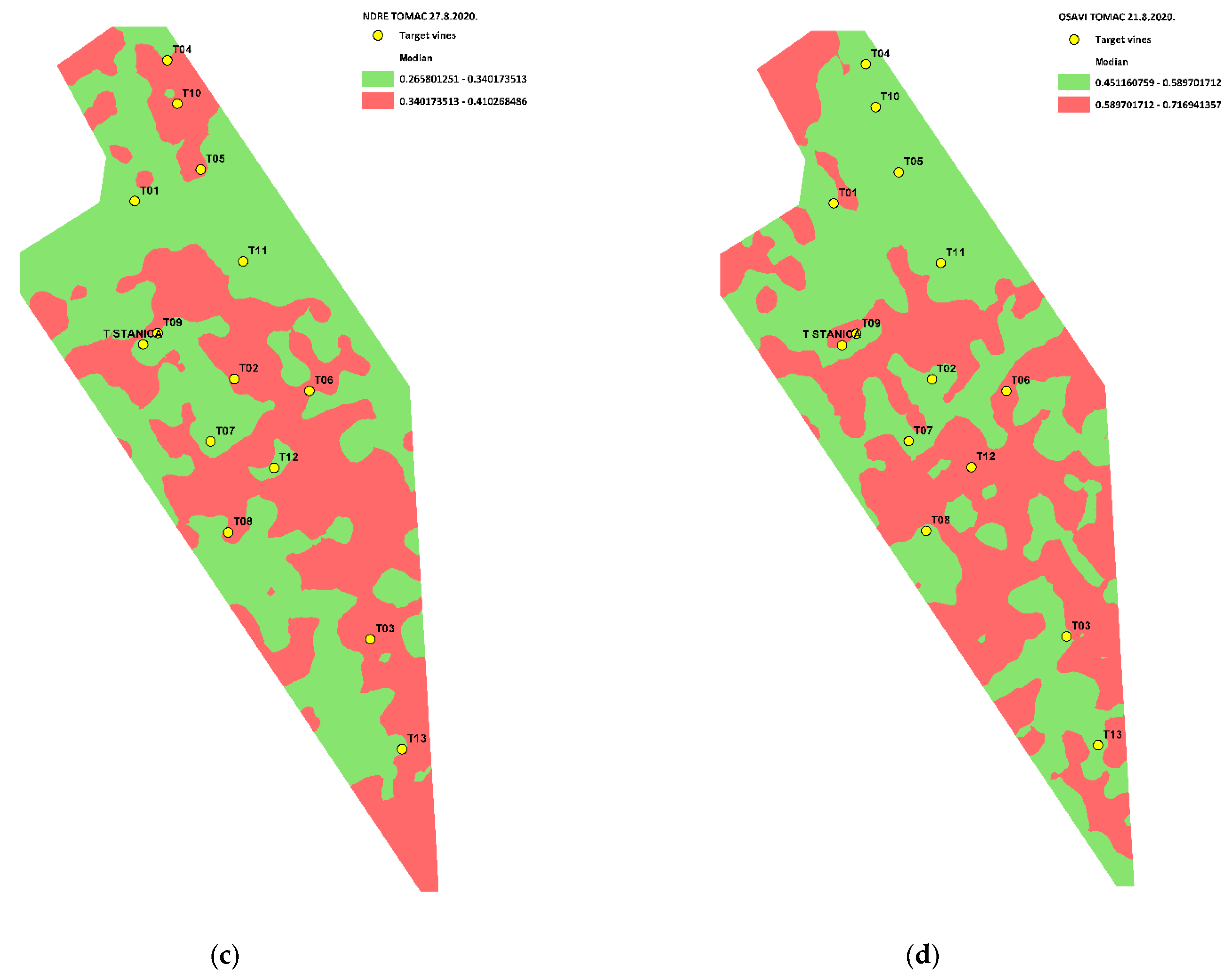
3.1. The Most Predictive Vegetation Index in 2019 and 2020–TOMAC Site

The collected data on grape quality components from the target vines in 2019 (n = 9) and 2020 (n = 13) were subjected to a clustering procedure using the K means cluster set for two clusters.

In this way, two clusters were obtained that were statistically significantly different in terms of sugar concentration (2019 and 2020), total titratable acidity (2019) and pH (2019). Within the first cluster were the target vines with a higher sugar concentration, lower total titratable acidity, and higher pH and that were characterised as having better grape quality components. Within the second cluster were the target vines with a lower sugar concentration, higher total titratable acidity, and lower pH and that were characterised as having inferior grape quality components (

Table 1. Results of the clustering of pinot noir grape quality components on target vines at the TOMAC site.

Grape Quality Components
2019 (n = 9)	F (1,7)	Sig.	First Cluster (n = 2)	Second Cluster (n = 7)
			M ± SD	M ± SD
Sugar concentration (°Oe)	8.365	0.023	91.00 ± 4.24	84.71 ± 2.36
Total titratable acidity (g/L)	10.647	0.014	5.56 ± 0.55	6.83 ± 0.47
pH	7.402	0.030	3.15 ± 0.02	3.09 ± 0.03
2020 (n = 13)	F (1,11)	Sig.	First cluster (n = 5)	Second cluster (n = 8)
			M ± SD	M ± SD
Sugar concentration (°Oe)	13.162	0.004	88.00 ± 3.39	81.00 ± 3.38
Total titratable acidity (g/L)	3.703	0.081	6.86 ± 0.85	7.66 ± 0.65
pH	1.776	0.210	3.09 ± 0.08	3.01 ± 0.11

Bold: Statistically significant components.

).

To determine the most predictive VI in relation to the grape quality components, an overlap was made between the classification structure of the vigour (categorical variable) and the cluster structure of the grape quality, which is shown in

Table 2. The overlap of classification structures obtained by quality clustering and vigour zoning on pinot noir target vines at the TOMAC site.

Vegetation Index	NDRE			NDVI			OSAVI
UAV image acquisition	GS 34	GS 36	GS 38	GS 34	GS 36	GS 38	GS 34	GS 36	GS 38
2019 (n = 9)
Number of equally classified vines	4	7	7	7	6	8	6	6	6
Percentage of equally classified vines	44%	78%	78%	78%	67%	89%	67%	67%	67%
2020 (n = 13)
Number of equally classified vines	8	7	11	8	8	8	8	6	8
Percentage of equally classified vines	62%	54%	85%	62%	62%	54%	62%	46%	62%

GS: growth stage; Bold: The most predictive VI.

.

Table 2 shows that the most predictive VI for grape quality zoning of pinot noir vineyards at the TOMAC site in 2019 was NDVI, with 89% overlap of classification structures at GS 38 (UAV image acquisition in September), while the least predictive was NDRE at GS 34 (UAV image acquisition in July).

In 2020, the most predictive VI was NDRE, with 85% overlap of classification structures at GS 38 (UAV image acquisition in September), while the least predictive was OSAVI at GS 36 (UAV image acquisition in August).

The generated vigour maps of the most and least predictive VIs at the TOMAC site in 2019 and 2020 are shown in Figure 1.

Based on the most predictive VI in 2019—the NDVI of GS 38—and the most predictive VI in 2020—the NDRE of GS 38—the statistical significance of the differences between the two vigour zones was tested using the averaged results for ten vegetative, yield, and grape components (2019:

Table 3. Descriptive statistical analysis and results of testing the statistical significance (SS) of differences between the two vigour zones for the chosen components at the TOMAC site in 2019, based on the most predictive VI: the NDVI of GS 38.

Analysed Variables	High-Vigour Target Vines (n = 6)		Low-Vigour Target Vines (n = 3)		SS of Differences (Average) Results/Ranks
	M ± SD (CV)	Shapiro–Wilk	M ± SD (CV)	Shapiro–Wilk	F	t (7)	Mann–Whitney U
Sugar concentration (°Oe)	84.33 ± 2.34 (2.77)	0.836	89.67 ± 3.79 (4.22)	0.855	1.514	−2.667 *
Total titratable acidity (g/L)	6.90 ± 0.49 (7.04)	0.898	5.86 ± 0.65 (11.01)	0.984	0.146	2.739 *
Yield (kg)	2.71 ± 0.61 (22.56)	0.860	1.56 ± 0.77 (49.32)	0.896	0.184	2.448 *

* p < 0.05; M = average value; SD = standard deviation; and CV = coefficient of variation; Bold: Statistically significant components; Grey background: test not used.

and Table S1; 2020:

Table 4. Descriptive statistical analysis and results of testing the statistical significance (SS) of differences between the two vigour zones for the chosen components at the TOMAC site in 2020, based on the most predictive VI: the NDRE of GS 38.

Analysed Variables	High-Vigour Target Vines (n = 8)		Low-Vigour Target Vines (n = 5)		SS of Differences (Average) Results/Ranks
	M ± SD (CV)	Shapiro–Wilk	M ± SD (CV)	Shapiro–Wilk	F	t (11)	Mann–Whitney U
Sugar concentration (°Oe)	81.13 ± 3.52 (4.34)	0.901	87.80 ± 3.63 (4.14)	0.914	0.015	−3.286 **
Total titratable acidity (g/L)	7.75 ± 0.62 (8.01)	0.924	6.73 ± 0.70 (10.40)	0.973	0.063	2.749 *

** p < 0.01; * p < 0.05; M = average value; SD = standard deviation; and CV = coefficient of variation; Bold: Statistically significant components; Grey background: test not used.

and Table S2).

In 2019, the two vigour zones differed significantly in the average results of the sugar concentration (homogeneous variance, t₍₇₎ = −2.667, p < 0.05), total titratable acidity (homogeneous variance, t₍₇₎ = 2.739, p < 0.05), and yield (homogeneous variance, t₍₇₎ = 2.448, p < 0.05), with vines from the low-vigour zone having a higher sugar concentration (M ± SD = 89.67 ± 3.79), lower total titratable acidity (M ± SD = 5.86 ± 0.65), and lower yield (M ± SD = 1.56 ± 0.77). The other measured vegetative, yield, and grape quality components that were not significantly different are listed in the Supplementary Materials (Table S1).

In 2020, the two vigour zones differed significantly in the average results of the sugar concentration (homogeneous variance, t₍₁₁₎ = −3.286, p < 0.01) and total titratable acidity (homogeneous variance, t₍₁₁₎ = 2.749, p < 0.05), with vines from the low-vigour zone having a higher sugar concentration (M ± SD = 87.80 ± 3.63) and lower total titratable acidity (M ± SD = 6.73 ± 0.70). The other measured vegetative, yield, and grape quality components that were not significantly different are listed in the Supplementary Materials (Table S2).

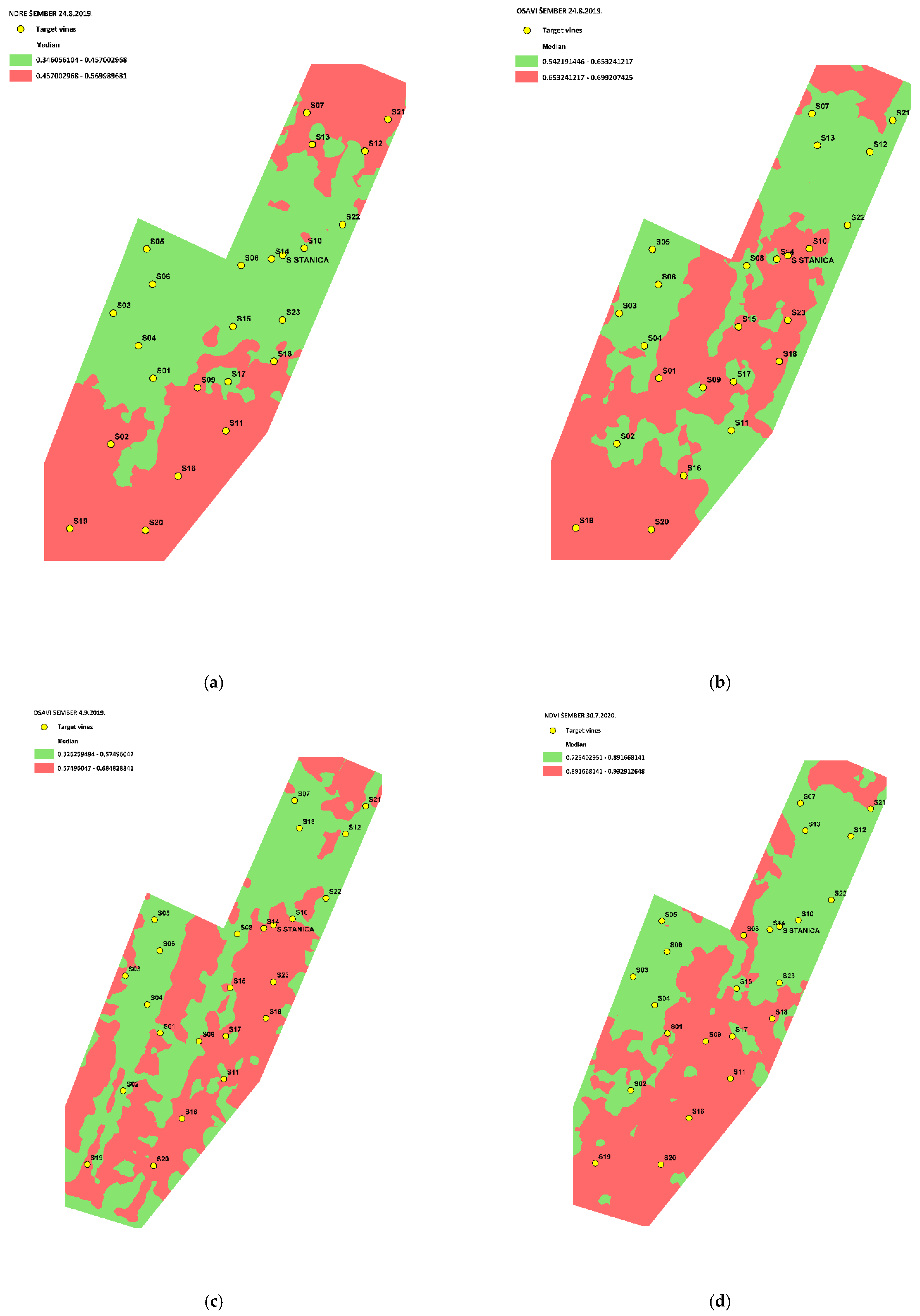
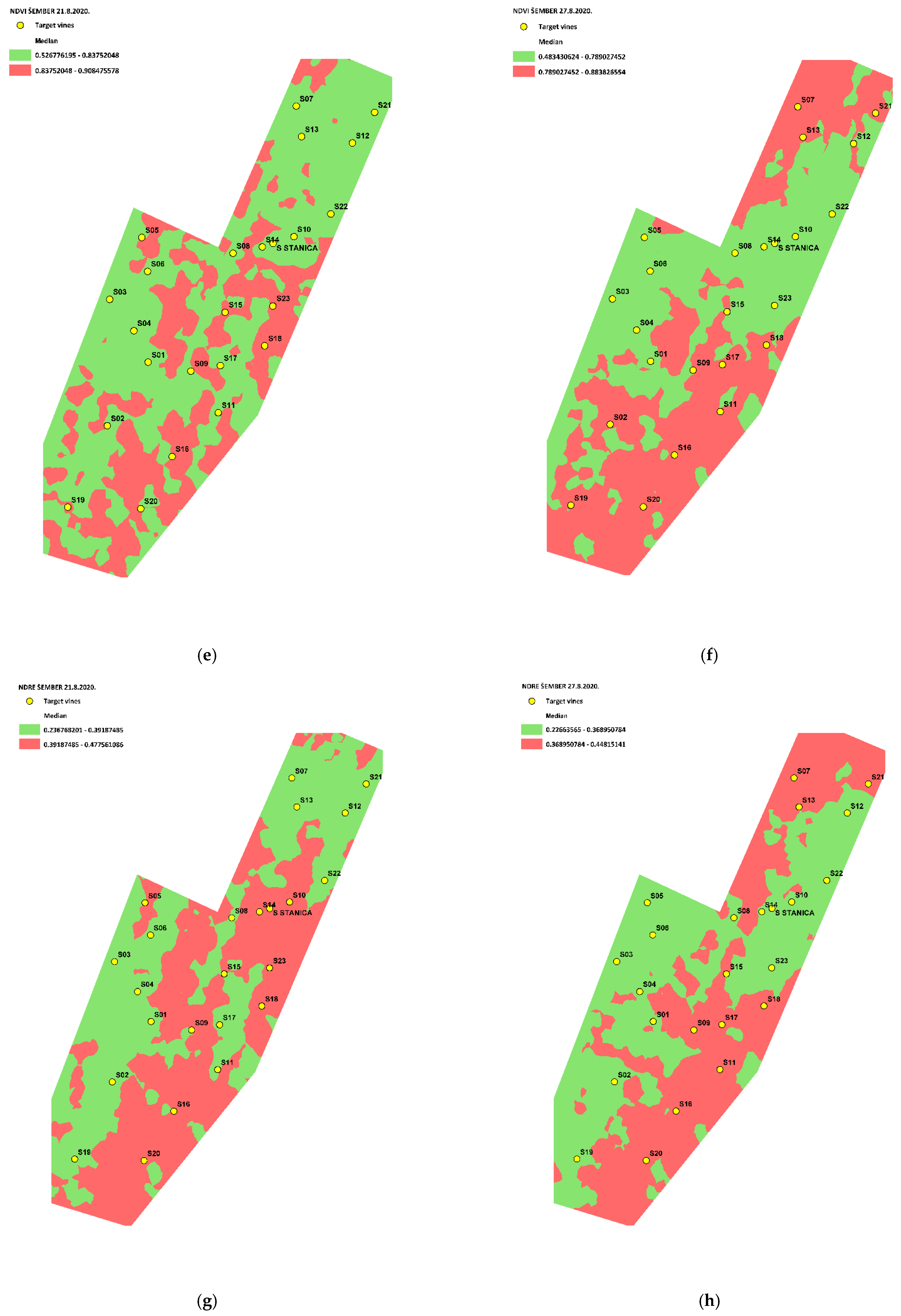
3.2. The Most Predictive Vegetation Index in 2019 and 2020–ŠEMBER Site

The collected data on grape quality components from the target vines in 2019 (n = 12) and 2020 (n = 22) were subjected to a clustering procedure using the K means cluster set for two clusters.

In this way, two clusters were obtained that were statistically significantly different in terms of sugar concentration (2019 and 2020), total titratable acidity (2019), and pH (2019 and 2020). Within the first cluster were the target vines with a lower sugar concentration, higher total titratable acidity, and lower pH and that were characterised as having inferior grape quality components. Within the second cluster were target vines with a higher sugar concentration, lower total titratable acidity, and higher pH and that were characterised as having better grape quality components (

Table 5. Results of the clustering of pinot noir grape quality components on target vines at the ŠEMBER site.

Grape Quality Components
2019 (n = 12)	F (1,10)	Sig.	First Cluster (n = 4)	Second Cluster (n = 8)
			M ± SD	M ± SD
Sugar concentration (°Oe)	32.502	0.000	75.75 ± 2.22	84.63 ± 2.67
Total titratable acidity (g/L)	10.146	0.010	9.84 ± 1.08	8.02 ± 0.86
pH	26.378	0.000	2.93 ± 0.02	3.07 ± 0.05
2020 (n = 22)	F (1,20)	Sig.	First cluster (n = 13)	Second cluster (n = 9)
			M ± SD	M ± SD
Sugar concentration (°Oe)	40.046	0.000	84.15 ± 3.02	94.22 ± 4.47
Total titratable acidity (g/L)	4.063	0.057	7.69 ± 1.84	6.27 ± 1.23
pH	8.492	0.009	3.07 ± 0.11	3.21 ± 0.11

M= average value; SD= standard deviation; Bold: Statistically significant components.

).

To determine the most predictive VI in relation to the grape quality components, an overlap was made between the classification structure of the vigour (categorical variable) and the cluster structure of the grape quality, which is shown in

Table 6. The overlap of classification structures obtained by quality clustering and vigour zoning on pinot noir target vines at the ŠEMBER site.

Vegetation Index	NDRE			NDVI			OSAVI
UAV image acquisition	GS 34	GS 36	GS 38	GS 34	GS 36	GS 38	GS 34	GS 36	GS 38
2019 (n = 12)
Number of equally classified vines	7	9	6	8	7	6	8	5	5
Percentage of equally classified vines	58%	75%	50%	67%	58%	50%	67%	42%	42%
2020 (n = 22)
Number of equally classified vines	16	15	15	19	15	15	17	16	16
Percentage of equally classified vines	73%	68%	68%	86%	68%	68%	77%	73%	73%

GS: growth stage. Bold: The most predictive VI.

.

Table 6 shows that the most predictive VI for the grape quality zoning of pinot noir vineyards at the ŠEMBER site in 2019 was NDRE, with 75% overlap of classification structures at GS 36 (UAV image acquisition in August), while the least predictive was OSAVI at GS 36 and 38 (UAV image acquisition in August and September).

In 2020, the most predictive VI was NDVI, with 86% overlap of classification structures at GS 34 (UAV image acquisition in July), while the least predictive were NDVI and NDRE at GS 36 and 38 (UAV image acquisition in August and September).

The generated vigour maps of the most and the least predictive VIs at the ŠEMBER site in 2019 and 2020 are shown in Figure 2.

Based on the most predictive VI in 2019—the NDRE of GS 36—and the most predictive VI in 2020—the NDVI of GS 34—the statistical significance of the differences between the two vigour zones was tested using the averaged results for ten vegetative, yield, and grape components (2019:

Table 7. Descriptive statistical analysis and results of testing the statistical significance (SS) of differences between the two vigour zones for the chosen components at the ŠEMBER site in 2019, based on the most predictive VI: the NDRE of GS 36.

Analysed Variables	High-Vigour Target Vines (n = 7)		Low-Vigour Target Vines (n = 5)		SS of Differences (Average) Results/Ranks
	M ± SD (CV)	Shapiro–Wilk	M ± SD (CV)	Shapiro–Wilk	F	t (10)	Mann–Whitney U
Sugar concentration (°Oe)	78.29 ± 3.55 (4.53)	0.729 **	86.40 ± 1.34 (1.55)	0.552 ***			0.000 **
Total titratable acidity (g/L)	9.32 ± 1.07 (11.49)	0.934	7.66 ± 0.83 (10.89)	0.914	0.115	2.872 *
pH	2.98 ± 0.07 (2.20)	0.805 *	3.08 ± 0.06 (2.07)	0.818			3.000 *
Leaf N content (% on a dry matter basis)	2.21 ± 0.12 (5.28)	0.926	2.01 ± 0.10 (4.94)	0.843	0.278	3.009 *

*** p < 0.001; ** p < 0.01; * p < 0.05; M = average value; SD = standard deviation; and CV = coefficient of variation; Bold: Statistically significant components; Grey background: test not used.

and Table S3; 2020:

Table 8. Descriptive statistical analysis and results of testing the statistical significance (SS) of the differences between the two vigour zones for the chosen components at the ŠEMBER site in 2020, based on the most predictive VI: the NDVI of GS 34.

Analysed Variables	High-Vigour Target Vines (n = 10)		Low-Vigour Target Vines (n = 12)		SS of Differences (Average) Results/Ranks
	M ± SD (CV)	Shapiro–Wilk	M ± SD (CV)	Shapiro–Wilk	F	t (20)	Mann–Whitney U
Sugar concentration (°Oe)	83.40 ± 3.06 (3.67)	0.974	92.33 ± 5.12 (5.55)	0.925	2.532	−4.831 ***
Total titratable acidity (g/L)	8.05 ± 1.93 (23.93)	0.768 **	6.33 ± 1.12 (17.78)	0.840 *			19.000 **
pH	3.05 ± 0.11 (3.54)	0.921	3.19 ± 0.11 (3.31)	0.957	0.034	−3.136 **
Leaf N content (% on a dry matter basis)	1.98 ± 0.10 (4.99)	0.978	1.86 ± 0.10 (5.14)	0.903	0.053	2.914 **

*** p < 0.001; ** p < 0.01; * p < 0.05; M = average value; SD = standard deviation; and CV = coefficient of variation. Bold: Statistically significant components; Grey background: test not used.

and Table S4).

In 2019, the two vigour zones differed significantly in the average results of the sugar concentration (Mann–Whitney U = 0.000, p < 0.01), total titratable acidity (homogeneous variance, t₍₁₀₎ = 2.872, p < 0.05), pH (Mann–Whitney U = 3.000, p < 0.05), and leaf N content (homogeneous variance, t₍₁₀₎ = 3.009, p < 0.05), with vines from the low-vigour zone having a higher sugar concentration (M ± SD = 86.40 ± 1.34), lower total titratable acidity (M ± SD = 7.66 ± 0.83), higher pH (M ± SD = 3.08 ± 0.06), and lower leaf N content (M ± SD = 2.01 ± 0.10). The other measured vegetative, yield, and grape quality components that were not significantly different are listed in the Supplementary Materials (Table S3).

In 2020, the two vigour zones differed significantly in the average results of the sugar concentration (homogeneous variance, t₍₂₀₎ = −4.831, p < 0.001), total titratable acidity (Mann–Whitney U = 19.000, p < 0.01), pH (homogeneous variance, t₍₂₀₎ = −3.136, p < 0.01), and leaf N content (homogeneous variance, t₍₂₀₎ = 32.914, p < 0.01), with vines from the low-vigour zone having a higher sugar concentration (M ± SD = 92.33 ± 5.12), lower total titratable acidity (M ± SD = 6.33 ± 1.12), higher pH (M ± SD = 3.19 ± 0.11), and lower leaf N content (M ± SD = 1.86 ± 0.10). The other measured vegetative, yield, and grape quality components that were not significantly different are listed in the Supplementary Materials (Table S4).

3.3. Economic Efficiency of Grape Quality Zoning and Selective Harvesting

3.3.1. Fixed and Variable Costs of Grape Quality Zoning and Selective Harvesting

The costs were divided into fixed and variable costs. All variable costs were standardised to an area of 1 ha, which was adjusted to the actual area of the vineyard at both sites in all the calculations of economic efficiency.

The cost structure table (

Table 9. The fixed and variable costs of quality zoning and selective harvesting.

Fixed Costs–Equipment Purchase Costs				PRICE (EUR)
DJI Phantom 4 Multispectral UAV				5600.00
Additional battery				160.00
Computer for data processing				1300.00
Software Pix4D				2600.00
DPO crew mandatory training for drone pilot				530.00
Training for the UAV image analysis and data processing (Pix4D fields)				1000.00
Insurance and registration of UAV				1000.00
			TOTAL	12,190.00
Variable Human Labour Costs (1 ha)	Time required	EUR/h	Quantity	PRICE (EUR)
Manual sampling on target vines	4	6.70	3	80.40
Education on the use of UAV	30	6.70	1	201.00
Education on the data processing	40	6.70	1	268.00
UAV data acquisition	3	6.70	3	60.30
Data processing and creation of quality zones	3	6.70	3	60.30
Selective harvesting	220	3.30	1	726.00
Extra costs of selective harvesting	50	3.30	1	165.00
			TOTAL	1561.00
Variable Service Costs	Area (ha)	EUR/ha		PRICE (EUR)
COMMERCIAL SERVICE–UAV image acquisition	1	400.00	3	1200.00
COMMERCIAL SERVICE–data processing	1	400.00	3	1200.00
			TOTAL	2400.00

Prices of equipment, human labour and services were relevant for the Croatian market and were collected from market research in April 2022. All prices were recalculated according to the exchange rate of 1 EUR = 7.5 HRK.

) shows that an investment of EUR 12,190.00 is required for the basic equipment and education for winegrowers to implement quality zonal management in their own vineyards. The variable costs were divided into variable human labour costs, which are incurred when the winegrower decides to purchase the equipment and start grape quality zoning and selective harvesting in his vineyard, and variable service costs, which are incurred when the winegrower decides to use the commercial service of a specialised company that, among other things, provides data processing and analysis with reports and recommendations for the winegrowers.

According to the initial results of this study regarding the terms of data collection and the number of required UAV image acquisitions, it is desirable to have three UAV image acquisitions during the growing season to obtain better data for grape quality zoning and selective harvesting; therefore, these costs were calculated accordingly.

3.3.2. Pinot Noir Wine Prices in the Plešivica Subregion

The market prices for pinot noir wines were obtained through market research in online stores of specialised wine shops for both of the wine producers in this research (

Table 10. Market prices of pinot noir wines from the Plešivica subregion.

Wine	Market (Retail) Price (EUR/Bottle 0.75 l)
Pinot noir Šember Vučjak *	20.00
Sparkling wine Šember Rose *	16.00
Pinot noir Tomac *	19.33
Sparkling wine Tomac Rose *	16.67
Pinot Noir Wine From the Plešivica Subregion
Pinot noir Ledić *	4.66
Pinot noir Filipec *	10.66
Pinot noir Braje *	11.33
Pinot noir Šoškić *	13.60
Average Market Price	10.07

* Source: Vrutak, available online: https://www.vrutak.hr/vino-domace (accessed on 10 April 2022). All prices were recalculated according to the exchange rate of 1 EUR = 7.5 HRK.

). In addition, the average market prices of pinot noir wine from the Plešivica PDO or the Western Continental Croatia PDO were calculated for the “regular” pinot noir wine price, as the winemakers in this research did not have this type of wine in their portfolio (Table 10).

3.3.3. Potential Revenues after Grape Quality Zoning and Selective Harvesting

The actual yields of harvested grapes from both sites and both years were used to calculate the potential revenues from wine production (

Table 11. Potential revenue increases from wine production after selective harvesting.

	TOMAC Site		ŠEMBER Site
Year	2019	2020	2019	2020
Vineyard area (ha)	0.33	0.33	0.65	0.65
Quantity of grapes harvested (kg)	1800	0.900	6570	4815
Amount of produced wine (l)	1260	1330	599	3371
Number of produced bottles (0.75 l) (pcs)	1680	1773	6132	4494
Average bottle price (EUR/bottle 0.75 l)	10.07	10.07	10.07	10.07
Sales revenue without selective harvesting (EUR)	16,917.60	17,854.11	61,749.24	45,254.58
Percentage of low-vigour zone (%)	61.97	54.33	49.47	47
Percentage of high-vigour zone (%)	38.03	45.67	50.53	53
Number of produced bottles from low-vigour zone (pcs)	1041	963	3034	2112
Number of produced bottles from high-vigour zone (pcs)	639	810	3098	2382
Wine price from low-vigour zone (EUR/bottle 0.75 l)	19.33	19.33	20	20
Wine price from high-vigour zone (EUR/bottle 0.75 l)	16.67	16.67	16	16
Total revenue from low-vigour zone (EUR)	20,122.53	18,614.79	60,680.00	42,240.00
Total revenue from high-vigour zone (EUR)	10,652.13	13,502.70	49,568.00	38,112.00
Potential sales revenue after selective harvesting (EUR)	30,774.66	32,117.49	110,248.00	80,352.00
Potential revenue increase after selective harvesting (EUR)	13,857.06	14,263.38	48,498.76	35,097.42
Potential revenue increase after selective harvesting (%)	45.03	44.41	43.99	43.68

All prices were recalculated according to the exchange rate of 1 EUR = 7.5 HRK.

). Based on the total quantity of grapes harvested at each site, the potential wine production was calculated using a 70% grape-to-wine ratio. The resulting potential wine volume (litres) was converted to the number of bottles produced (0.75 litres per bottle). Then, the total number of bottles was divided according to the percentage of the area of the high- and low-vigour zones based on the most predictive VI to obtain the number of bottles that could be produced from the grapes of each vigour zone. In this way, it was possible to calculate the potential sales revenues from the production of two wine types based on grape quality zoning and selective harvesting from the two different vigour zones. The wine prices used for the calculation of the potential revenues are taken from Table 10.

Table 11 shows that the potential sales revenues from wine production increased after selective harvesting at both sites. It shows that the potential revenue increase is 43.68 to 45.03% higher than the total revenue that can be obtained from wine production without selective harvesting. The increase in potential revenue depends mainly on the type of wine produced. This high percentage of increase in revenue in the production of two types of wine—still and sparkling—was observed at both sites (TOMAC and ŠEMBER). Both vineyard vigour zones were suitable for the production of high-quality wines. The grapes from the high-vigour zones were suitable for the production of sparkling wine due to the lower sugar concentration and the higher total titratable acidity, while the grapes from the low-vigour zones were suitable for the production of high-quality still wines. Both types of wine can achieve high bottle prices in the marketplace, so grape quality zoning and selective harvesting are useful tools for maximising these benefits.

A differential analysis (

Table 12. Differential analysis between two alternatives: to adopt or not to adopt quality zoning and selective harvesting.

TOMAC Site
	S1				S2
	A1	A2	Differential Amount	A2 Is:	A1	A2	Differential Amount	A2 Is:
Sales revenue (EUR)	16,917.60	30,774.66	13,857.06	higher	16,917.60	30,774.66	13,857.06	higher
Variable costs (EUR)	0.00	829.36	829.36	higher	0.00	2694.03	2694.03	higher
Fixed costs (EUR)	0.00	12,190.00	12,190.00	higher	0.00	0.00	0.00	equal
Profit (EUR)	16,917.60	17,755.30	837.70	higher	16,917.60	28,080.63	11,163.03	higher
ŠEMBER Site
	S1				S2
	A1	A2	Differential Amount	A2 Is:	A1	A2	Differential Amount	A2 Is:
Sales revenue (EUR)	61,749.24	110,248.00	48,498.76	higher	61,749.24	110,248.00	48,498.76	higher
Variable costs (EUR)	0.00	1178.80	1178.80	higher	0.00	2979.15	2979.15	higher
Fixed costs (EUR)	0.00	12,190.00	12,190.00	higher	0.00	0.00	0.00	equal
Profit (EUR)	61,749.24	96,879.20	35,129.96	higher	61,749.24	107,268.85	45,519.61	higher

All prices were recalculated according to the exchange rate of 1 EUR = 7.5 HRK.

) was conducted to determine the difference between two alternatives: to adopt (A2) or not to adopt (A1) grape quality zoning and selective harvesting. Two possible scenarios were also used: the winegrower performs grape quality zoning himself (S1), and the winegrower uses a commercial service for grape quality zoning (S2). Variable costs (costs for manual sampling and selective harvesting) were recalculated according to the vineyard area, while the 2019 sales revenue data were used for both winegrowers.

As shown in the differential analysis (Table 12), the profit from selective harvesting (A2) was higher under both scenarios and at both sites, despite higher costs. Using a commercial service for grape quality zoning yields even higher profits, as expected, but is also a less risky option for winegrowers, as they would not need to purchase and maintain equipment or pay attention to the proper execution of UAV flights, data processing, or interpretation, as these operations require specific experience and training.

4. Discussion

A two-year study on the possibility of using three different VIs—NDVI, NDRE, and OSAVI—for grape quality zoning has shown that VIs are effective tools for assessing the vigour and variability in small pinot noir vineyards in the Plešivica subregion, and they can successfully describe yield and grape quality components and link them to the results of spectral measurements. However, there are differences in the effectiveness of estimating the relationship between vigour, yield, and grape quality components, depending on the VI used and on the grapevine’s GS at the time that the multispectral UAV images are acquired.

OSAVI, the least used VI in previous studies, also proved to be the least predictive VI in this study for delineating vigour zones and grape quality zoning of vineyards. OSAVI was not the most predictive VI for delineating grape quality zones at any grapevine GS or any study site. These results are consistent with previous studies in which OSAVI was used mainly to estimate the nitrogen content in grapevines [45] for targeted nitrogen fertiliser applications. In previous studies, OSAVI was not used exclusively as a VI for the delineation of vigour zones, and according to the results of this study, its use would not provide sufficient results to successfully link vigour and grape quality components as a basis for grape quality zoning and selective harvesting. Further research that might be considered in the use of OSAVI could involve the processing of image data and the preparation of images acquired with the multispectral camera. OSAVI, as a soil-adapted VI that eliminates the influence of soil on vegetation analysis (i.e., analysis of nitrogen and chlorophyll content and estimation of the amount of aboveground cover) and uses a soil adjustment factor in the calculation (L = 0.16) [46,47], may not be suitable for use with images where row segmentation from the soil has been performed and where grapevine vegetation and soil data are already separated. The researchers who used OSAVI on grapevines [45,48] did not perform row segmentation in their studies.

NDVI has been the most commonly used VI in previous research for delineating vigour zones and grape quality zoning of vineyards, and this study also found NDVI to be the most predictive VI at both sites and in both years, but at different grapevine GSs (2019 at the TOMAC site: GS 38; 2020 at the ŠEMBER site: GS 34). Since most previous studies were conducted mainly with one-time UAV or satellite data collection for delineating vigour and grape quality zones, usually during the period corresponding to grape GS 36 (the beginning of sugar accumulation, or closely before or after veraison [4,5,7,8,9,10,11,13,14,16,18,49]), the results of this study are consistent with these previous studies. Other previous studies [6,12,15,17,39,50] were conducted at several different periods of UAV or satellite data acquisition during the growing season. Fiorillo et al. [6] used three different image acquisition periods (June–August) and concluded that data acquisition at an earlier stage of grape ripening (beginning of sugar accumulation or earlier) showed the best ability to delineate grape quality zones in terms of measured grape quality components. This was confirmed in this study at the ŠEMBER site (2020). Moreover, Oldoni et al. [17] concluded that NDVI maps obtained at the later stages of grape ripening and under normal climatic conditions (without extreme rainfall) were useful for grape quality zoning, allowing selective harvesting, which was also confirmed in this study at the TOMAC site (2019). Ledderhof et al. [12] reported that it is not possible to precisely determine the best time for UAV data acquisition. Their study, conducted in a pinot noir vineyard with four different UAV data acquisition periods (29 May, 1 July, 29 July, and 21 August), showed the possibility of delineating vigour zones and grape quality zones based on NDVI, but they did not find an ideal UAV data acquisition period that would be the most suitable for predicting grape quality components at harvest, which was also confirmed in this study. In conclusion, NDVI proved to be a very good tool for delineating grape quality zones, but further research is needed on the ideal UAV data acquisition period depending on the climatic conditions during the growing season. The stability of vigour and grape quality zones in vineyards has also been studied [12,51,52], and these authors concluded that more than two years of consecutive monitoring and grape quality zoning in the same vineyard are needed for the results to be reliable enough for practical application. These conclusions also apply to the present study, which offers a perspective for future multi-year research.

NDRE proved to be the most predictive VI in this study at both sites and in both years, but at different grapevine GSs (2019 at the ŠEMBER site: GS 36; 2020 at the TOMAC site: GS 38). Since NDRE was developed relatively recently [42], its practical value for grape quality zoning is not as well studied, but its use has been previously confirmed for the delineation of vigour zones in later grapevine GSs, i.e., grape ripening [53], which is also confirmed in this study. At both sites, the use of NDRE to delineate grape quality zones at later grapevine GSs was successful, and the zones were statistically significant. It can be said that the use of NDRE for the grape quality zoning of pinot noir vineyards is sufficiently predictive for purposes such as selective harvesting in the growing season in which the data are collected. As mentioned earlier, multi-year monitoring would be helpful to increase the accuracy of grape quality zoning and allow the introduction of other precision tools for viticulture. In addition, the use of new approaches (machine learning and artificial intelligence) [54] and different grape quality and yield estimation devices [55] could also increase the accuracy of grape quality zoning.

The economic efficiency of grape quality zoning and selective harvesting was evident in this study. It is recommended that winegrowers adopt grape quality zoning and selective harvesting as a tool to maximise the effects of variability by producing different wine types from the same grape variety and in the same vineyard. According to previous research by Bramley et al. [24], a possible sales revenue increase after producing wine with two different wine quality categories can provide a USD 30,791.00 (EUR 29,325.00) higher gross retail value for production per ha, while the calculations in this study are even higher—about EUR 14,000.00/0.33 ha (TOMAC site) and about EUR 40,000.00/0.65 ha (ŠEMBER site). Considering the fact that both sites were small, family-owned boutique wineries and the selling price of their wines was above average, it can be said that selective harvesting is a good approach, as the transition to “super-premium” wines was made for both grape quality zones [29,30]. Moreover, the calculations in this study showed that the transition to “super-premium” wines from the entire vineyard area in both sites can increase wine prices by EUR 5–10 per bottle. Bramley et al. [29] reported a potential revenue increase of USD 5 per bottle, but the revenue increase was highly dependent on the wine selling prices [30] of particular winery and could not be generalised. It can be said that selective harvesting is a good tool for small boutique wineries with a good market position and good wine prices.

Differential analysis has shown that both scenarios for grape quality zoning result in a higher profit from selective harvesting at both sites, despite the higher investment costs. This makes the investment in grape quality zoning financially and economically feasible [56]. These results also provide a pathway for the adoption of innovation, as the “with or without” scenario is critical in deciding whether to adopt an innovation that maximises profit while making minor adjustments to the production system [2]. As expected, the use of a commercial service for grape quality zoning in this study yielded even higher profits, which is consistent with the statement of Swinton and Ahmad [45]: “When services are custom hired, virtually all costs are monetary. So where financial benefits exceed custom hire costs, we can conclude that a practice is profitable”. Commercial services are also a less risky option for winegrowers because they do not have to purchase and maintain equipment or pay attention to proper UAV flight execution, data processing, and data interpretation. These activities require specialised training and experience, which were mentioned in Swinton and Ahmad [44] as unexpected monetary and non-monetary costs of the technology.

5. Conclusions

A two-year study using three different VIs—NDVI, NDRE, and OSAVI—for grape quality zoning has shown that VIs are effective tools for assessing vineyard vigour and variability in small pinot noir vineyards in the Plešivica subregion, and they can successfully link the results of spectral measurements to yield and grape quality components.

OSAVI, which was the least used index in previous studies, also proved to be the least predictive index in this study for delineating vigour zones and grape quality zoning of vineyards.

NDVI and NDRE showed very useful results when used to delineate vigour zones and grape quality zoning of vineyards. Nevertheless, multi-year monitoring of vineyards is needed to increase the accuracy of grape quality zones and to define the ideal grapevine GS for UAV image acquisition that corresponds best with grape quality components for a given region/vineyard/grape variety. NDRE proved to be the most predictive VI at later grapevine GSs (36–38), while NDVI was the most predictive in an early grapevine GS (34) and before harvest (38).

As mentioned previously, the economic efficiency of grape quality zoning and selective harvesting was evident in this study. The potential sales revenue from the production of “super-premium” wines after selective harvesting was 43.68 to 45.03% higher than the total revenue that could be generated from the production of “quality” wines at both sites. Considering the fact that both wineries were small, family-owned boutique wineries and the selling prices of their wines were above average, the important takeaway is that they can use high- and low-quality zones for the production of two types of “super-premium” wines—still and sparkling.

In terms of investment, both scenarios of using grape quality zoning resulted in higher profits, despite the higher costs required to implement grape quality zoning and selective harvesting. Using a commercial service provider for grape quality zoning resulted in higher profits and lower risks for the winegrower.

Further research could be considered for the use of OSAVI on images where row segmentation has already been performed and where the grapevine vegetation and soil data are already separated. In addition, the ideal UAV data acquisition period for grape quality zoning needs to be studied. This could be combined with other available technologies (i.e., hand-held multispectral cameras, soil moisture sensors, weather stations) or new approaches (machine learning and artificial intelligence) to enable more reliable practical application of grape quality zoning and selective harvesting to increase economic efficiency and maximise the profits from wine production.

References

1. Bramley, R.G.V. 12—Precision Viticulture: Managing vineyard variability for improved quality outcomes. In Managing Wine Quality; Reynolds, A.G., Ed.; Woodhead Publishing: Cambridge, UK, 2010; pp. 445–480. [Google Scholar] [CrossRef]
2. Maynard, H.D. An Economic Analysis of Precision Viticulture, Fruit, and Pre Release Wine Pricing across Three Western Australian Cabernet Sauvignon Vineyards. Ph.D. Thesis, Department of Environment and Agriculture, Curtin University, Perth, Australia, 2015. [Google Scholar]
3. Steyn, J.; Aleixandre-Tudo, J.L.; Aleixandre, J.L. Grapevine Vigour and Within-Vineyard Variability: A Review. Int. J. Sci. Eng. Res. 2016, 7, 1056–1065. [Google Scholar]
4. Johnson, L.F.; Bosch, D.F.; Williams, D.C.; Lobitz, B.M. Remote sensing of vineyard management zones: Implications for wine quality. Appl. Eng. Agric. 2001, 17, 557–560. [Google Scholar] [CrossRef]
5. Martínez-Casasnovas, J.A.; Agelet-Fernandez, J.; Arnó, J.; Ramos, C. Analysis of vineyard differential management zones and relation to vine development, grape maturity and quality. Span. J. Agric. Res. 2012, 10, 326–337. [Google Scholar] [CrossRef] [Green Version]
6. Fiorillo, E.; Crisci, A.; De Filippis, T.; Di Gennaro, S.F.; Di Blasi, S.; Matese, A.; Primicerio, J.; Vaccari, F.P.; Genesio, L. Airborne high-resolution images for grape classification: Changes in correlation between technological and late maturity in Sangiovece vineyard in Central Italy. Aust. J. Grape Wine Res. 2012, 18, 80–90. [Google Scholar] [CrossRef]
7. Filippetti, I.; Allegro, G.; Valentini, G.; Pastore, C.; Colucci, E.; Intrieri, C. Influence of vigour on vine performance and berry composition of cv. Sangiovese (Vitis vinifera L.). J. Int. Des Sci. De La Vigne Et Du Vin 2013, 47, 21–33. [Google Scholar] [CrossRef] [Green Version]
8. Santesteban, L.G.; Guillaume, S.; Royo, J.B.; Tisseyre, B. Are precision agriculture tools and methods relevant at the whole-vineyard scale? Precis. Agric. 2013, 14, 2–17. [Google Scholar] [CrossRef] [Green Version]
9. Urretavizcaya, I.; Santesteban, L.G.; Tisseyre, B.; Guillaume, S. Oenological significance of vineyard management zones delineated using early grape sampling. Precis. Agric. 2014, 15, 111–129. [Google Scholar] [CrossRef] [Green Version]
10. Bonilla, I.; Martinez de Toda, F.; Martinez-Casanovas, J.A. Vine vigour, yield and grape quality assessment by airborne remote sensing over three years: Analysis of unexpected relationships in cv. Tempranillo. Span. J. Agric. Res. 2015, 13, e0903. [Google Scholar] [CrossRef]
11. Ortega-Blu, R.; Molina, M. Evaluation of vegetation indices and apparent soil electrical conductivity for site-specific vineyard management in Chile. Precis. Agric. 2016, 17, 434–450. [Google Scholar] [CrossRef]
12. Ledderhof, D.; Brown, R.; Reynolds, A.; Jollineau, M. Using remote sensing to understand Pinot noir vineyard variability in Ontario. Can. J. Plant Sci. 2016, 96, 89–108. [Google Scholar] [CrossRef]
13. Gatti, M.; Garavani, A.; Vercesi, A.; Poni, S. Ground-truthing of remotely sensed within-field variability in a cv. Barbera plot for improving vineyard management. Aust. J. Grape Wine Res. 2017, 23, 399–408. [Google Scholar] [CrossRef]
14. Matese, A.; Di Gennaro, S.; Miranda, C.; Berton, A.; Santesteban, L. Evaluation of spectral-based and canopy-based vegetation indices from UAV and Sentinel 2 images to assess spatial variability and ground vine parameters. Adv. Anim. Biosci. 2017, 8, 817–822. [Google Scholar] [CrossRef]
15. Pastonchi, L.; Di Gennaro, S.F.; Toscano, P.; Matese, A. Comparison between satellite and ground data with UAV-based information to analyse vineyard spatio-temporal variability. OENO One 2020, 54, 919–934. [Google Scholar] [CrossRef]
16. Ferrer, M.; Echeverria, G.; Pereyra, G.; Gonzales-Neves, G.; Pan, D.; Miras-Avalos, J.M. Mapping vineyard vigour using airborne remote sensing: Relations with yield, berry composition and sanitary status under humid conditions. Precis. Agric. 2020, 21, 178–197. [Google Scholar] [CrossRef]
17. Oldoni, H.; Costa, B.R.S.; Bognola, I.A.; de Souza, C.R.; Bassoi, L.H. Homogeneous zones of vegetation index for characterizing variability and site-specific management in vineyards. Sci. Agric. 2021, 78, e20190243. [Google Scholar] [CrossRef]
18. Reynolds, A.G.; Brown, R.; Jollineau, M.; Shemrock, A.; Lee, H.; Dorin, B.; Shabanian, M.; Meng, B. Viticultural Mapping by UAVs, Part 2 Applying Unmanned Aerial Vehicles in Viticulture. The Free Library. Wines Vines. 2018. Available online: https://www.thefreelibrary.com/Viticultural+Mapping+by+UAVs%2c+Part+2%3a+Applying+unmanned+aerial…-a0546959785 (accessed on 10 March 2021).
19. Poni, S.; Gatti, M.; Palliotti, A.; Dai, Z.; Duchêne, E.; Truong, T.T.; Ferrara, G.; Matarrese, A.; Gallotta, A.; Bellincontro, A.; et al. Grapevine quality: A multiple choice issue. Sci. Hortic. 2017, 234, 445–462. [Google Scholar] [CrossRef] [Green Version]
20. Lambert, D.M.; Lowenberg-DeBoer, J.; Griffin, T.W.; Peone, J.; Payne, T.; Daberkow, S.G. Adoption, Profitability, and Making Better Use of Precision Farming Data; Staff Papers 28615; Purdue University, Department of Agricultural Economics: West Lafayette, Indiana, 2004; Available online: https://ageconsearch.umn.edu/record/28615 (accessed on 13 February 2021).
21. Tisseyre, B.; Taylor, J.A. An overview of methodologies and technologies for implementing precision agriculture in viticulture. In Proceedings of the XII Congresso Brasileiro de Vitivinicultura e Enologia, Bento Goncavles, RS, Brasil, 22–24 September 2008. [Google Scholar]
22. Matese, A.; Di Gennaro, S.F. Practical Applications of a Multisensor UAV Platform Based on Multispectral, Thermal and RGB High Resolution Images in Precision Viticulture. Agriculture 2018, 8, 116. [Google Scholar] [CrossRef] [Green Version]
23. Andújar, D.; Moreno, H.; Bengochea-Guevara, J.; De Castro, A.; Ribeiro, A. Aerial imagery or on-ground detection? An economic analysis for vineyard crops. Comput. Electron. Agric. 2019, 157, 351–358. [Google Scholar] [CrossRef]
24. Bramley, R.G.V.; Pearse, B.; Chamberlain, P. Being profitable precisely—A case study of precision viticulture from Margaret River. Aust. New Zealand Grapegrow. Winemak. 2003, 84–87. [Google Scholar]
25. Proffit, T.; Malcom, A. Zonal vineyard management through airborne remote sensing. Aust. New Zealand Grapegrow. Winemak. 2005, 22–31. [Google Scholar]
26. Joint Research Centre (JRC) of the European Commission; Monitoring Agriculture ResourceS (MARS) Unit H04; Pablo, J.; Zarco-Tejada, P.J.; Hubbard, N.; Loudjani, P. Precision Agriculture: An Opportunity for EU Farmers—Potential Support with the CAP 2014-2020. European Parliamnet, Directorate-General for Internal Policies, 2014. Available online: https://www.europarl.europa.eu/RegData/etudes/note/join/2014/529049/IPOL-AGRI_NT%282014%29529049_EN.pdf (accessed on 13 February 2021).
27. Grgić, Z.; Očić, V.; Šakić Bobić, B. Troškovi i Kalkulacije u Agrobiznisu; Internal Students Book; Faculty of Agriculture: Zagreb, Croatia, 2011. [Google Scholar]
28. Bramley, R.G.V.; Proffitt, A.P.B.; Hinze, C.J.; Pearse, B.; Hamilton, R.P. Generating benefits from precision viticulture through selective harvesting. In Proceedings of the 5th European Conference on Precision Agriculture-Precision agriculture ’05, Uppsala, Sweden, 9–12 June 2005; pp. 891–898. [Google Scholar] [CrossRef]
29. Bramley, R.G.V.; Ouzman, J.; Thornton, C. Selective harvesting is a feasible and profitabile strategy even when grape and wine production is geared towards large fermentation volumes. Aust. J. Grape Wine Res. 2011, 17, 298–305. [Google Scholar] [CrossRef]
30. Rousseau, J.; Lefevre, V.; Douche, H.; Poilve, H.; Habimana, T. Oenoview®: Remote Sensing in Support of Vineyard Profitability and Wine Quality. Acta Hortic. 2013, 978, 139–148. [Google Scholar] [CrossRef]
31. Maletić, E.; Karoglan Kontić, J.; Pejić, I. Vinova Loza Ampelografija, Ekologija, Oplemenjivanje; Školska Knjiga: Zagreb, Croatia, 2008. [Google Scholar]
32. Mirošević, N.; Alpeza, I.; Bolić, J.; Brkan, B.; Hruškar, M.; Husnjak, S.; Jelaska, V.; Karoglan Kontić, J.; Maletić, E.; Mihaljević, B.; et al. Atlas Hrvatskog Vinogradarstva i Vinarstva; Golden Marketing—Tehnička Knjiga: Zagreb, Croatia, 2009. [Google Scholar]
33. Coombe, B.G. Adoption of a system for identifying grapevine growth stages. Aust. J. Grape Wine Res. 1995, 1, 100–110. [Google Scholar] [CrossRef]
34. Delenne, C.; Durrieu, S.; Rabatel, G.; Deshayes, M. From pixel to vine parcel: A complete methodology for vineyard delineation and characterization using remote-sensing data. Comput. Electron. Agric. 2010, 70, 78–83. [Google Scholar] [CrossRef] [Green Version]
35. Comba, L.; Gay, P.; Primicerio, J.; Ricauda Aimonino, D. Vineyard detection from unmanned aerial systems images. Comput. Electron. Agric. 2015, 114, 78–87. [Google Scholar] [CrossRef]
36. Nolan, A.P.; Park, S.; O’Connell, M.; Fuentes, S.; Ryu, D.; Chung, H. Automated detection and segmentation of vine rows using high resolution UAS imagery in a commercial vineyard. In Proceedings of the 21st International Congress on Modelling and Simulation, MODSIM 2015, Broadbeach, Queensland, Australia, 29 November–4 December 2015; pp. 1406–1412. [Google Scholar]
37. Primicerio, J.; Gay, P.; Ricauda Aimonino, D.; Comba, L.; Matese, A.; Di Gennaro, S. NDVI-based vigour maps production using automatic detection of vine rows in ultra-high resolution aerial images. In Precision Agriculture ’15, Proceedings of 10th European Conference on Precision Agriculture, Israel, 12–16 July 2015; Stafford, J.V., Ed.; Wageningen Academic Publishers: Wageningen, The Netherlands, 2015; pp. 465–470. [Google Scholar] [CrossRef]
38. De Castro, A.I.; Jiménez-Brenes, F.M.; Torres-Sánchez, J.; Peña, J.M.; Borra-Serrano, I.; López-Granados, F. 3-D Characterization of Vineyards Using a Novel UAV Imagery-Based OBIA Procedure for Precision Viticulture Applications. Remote Sens. 2018, 10, 584. [Google Scholar] [CrossRef] [Green Version]
39. Pádua, L.; Marques, P.; Adão, T.; Guimarães, N.; Sousa, A.; Peres, E.; Sousa, J. Vineyard Variability Analysis through UAV-Based Vigour Maps to Assess Climate Change Impacts. Agronomy 2019, 9, 581. [Google Scholar] [CrossRef] [Green Version]
40. Campos, J.; García-Ruíz, F.; Gil, E. Assessment of Vineyard Canopy Characteristics from Vigour Maps Obtained Using UAV and Satellite Imagery. Sensors 2021, 21, 2363. [Google Scholar] [CrossRef] [PubMed]
41. Rouse, J.W.; Haas, R.H.; Schell, J.A.; Deering, D.W. Monitoring vegetation systems in the Great Plains with ERTS. In Proceedings of the 3rd ERTS Symposium, Washington, DC, USA, 10–14 December 1973; NASA: Washington, DC, USA NASA SP-351. ; pp. 309–317. [Google Scholar]
42. Buschmann, C.; Nagel, E. In Vivo Spectroscopy and Internal Optics of Leaves as Basis for Remote Sensing of Vegetation. Int. J. Remote Sens. 1993, 14, 711–722. [Google Scholar] [CrossRef]
43. Rondeaux, G.; Steven, M.; Baret, F. Optimization of Soil-Adjusted Vegetation Indices. Remote Sens. Environ. 1996, 55, 95–107. [Google Scholar] [CrossRef]
44. Swinton, S.M.; Ahmad, M. Returns to Farmer Investments in Precision Agriculture Equipment and Services. In Proceedings of the Third International Conference on Precision Agriculture, Minneapolis, MN, USA, 23–26 June 1996; American Society of Agronomy, Crop Science Society of America, Soil Science Society of America: Madison, WI, USA, 1996; pp. 1009–1018. [Google Scholar] [CrossRef]
45. Kidman, C.; Pagay, V.; Jenkins, A. Optimizing Water Use Efficiency for Improved Wine Quality in Coonawarra Vineyards Using Remote Sensing Technologies—Season 2. Final Report. 2017. Available online: https://coonawarra.org/wp-content/uploads/2017/06/CWGI-Final-report-310517.pdf (accessed on 12 April 2021).
46. Xue, J.; Su, B. Significant Remote Sensing Vegetation Indices: A Review of Developments and Application. J. Sens. 2017, 2017, 1353691. [Google Scholar] [CrossRef] [Green Version]
47. Fern, R.; Foxley, E.; Bruno, A.; Morrison, M. Suitability of NDVI and OSAVI as estimators of green biomass and coverage in a semi-arid rangeland. Ecol. Indic. 2018, 94, 16–21. [Google Scholar] [CrossRef]
48. Soubry, I.; Patias, P.; Tsioukas, V. Monitoring vineyards with UAV and multi-sensors for the assessment of water stress and grape maturity. J. Unmanned Veh. Syst. 2016, 5, 37–50. [Google Scholar] [CrossRef] [Green Version]
49. Candiago, S.; Remondino, F.; De Giglio, M.; Dubbini, M.; Gattelli, M. Evaluating Multispectral Images and Vegetation Indices for Precision Farming Applications from UAV Images. Remote Sens. 2015, 7, 4026–4047. [Google Scholar] [CrossRef] [Green Version]
50. Lamb, D.W.; Weedon, M.M.; Bramley, R.G.V. Using remote sensing to map grape phenolics and colour in a cabernet sauvignon vineyard—The impact of image resolution and vine phenology. Aust. J. Grape Wine Res. 2004, 10, 46–54. [Google Scholar] [CrossRef] [Green Version]
51. Bonilla, I.; Martínez de Toda, F.; Martínez-Casasnovas, J.A. Vineyard zonal management for grape quality assessment by combining airborne remote sensed imagery and soil sensors. In Remote Sensing for Agriculture, Ecosystems, and Hydrology XVI, Proceedings of SPIE Remote Sensing, Amsterdam, Netherlands, 11 November 2014; SPIE Digital Library: Bellingham, WA, USA, 2014. [Google Scholar] [CrossRef] [Green Version]
52. Kazmierski, M.; Glémas, P.; Rousseau, J.; Tisseyre, B. Temporal stability of within-field patterns of NDVI in non irrigated Mediterranean vineyards. OENO One 2011, 45, 61–73. [Google Scholar] [CrossRef]
53. D‘Urso, M.G.; Rotondi, A.; Gagliardini, M. UAV low-cost system for evaluating and monitoring the growth parameters of crops. In ISPRS Annals of the Photogrammetry, Remote Sensing and Spatial Information Sciences 2018, IV-5, Proceedings of ISPRS TC V Mid-term Symposium “Geospatial Technology—Pixel to People”, Dehradun, India, 20–23 November 2018; Kumar, A.S., Saran, S., Padalia, H., Eds.; ISPRS: Hannover, Germany, 2018; pp. 405–413. [Google Scholar]
54. Sozzi, M.; Cantalamessa, S.; Cogato, A.; Kayad, A.; Marinello, F. Grape yield spatial variability assessment using YOLOv4 object detection algorithm. In Proceedings of the 13th European Conference on Precision Agriculture, Budapest, Hungary, 19–22 July 2021. [Google Scholar] [CrossRef]
55. Sozzi, M.; Cogato, A.; Boscaro, D.; Kayad, A.; Tomasi, D.; Marinello, F. Validation of a commercial optoelectronics device for grape quality analysis. In Proceedings of the 13th European Conference on Precision Agriculture, Budapest, Hungary, 19–22 July 2021. [Google Scholar] [CrossRef]
56. Shockley, J.; Mark, T.; Dillon, C. Educating producers on the profitability of precision agriculture technologies. Adv. Anim. Biosci. 2017, 8, 724–727. [Google Scholar] [CrossRef]
Figure 1. (a) NDVI vigour map of GS 38 in 2019 (the most predictive 2019 map); (b) NDRE vigour map of GS 34 in 2019 (the least predictive 2019 map); (c) NDRE vigour map of GS 38 in 2020 (the most predictive 2020 map); and (d) OSAVI vigour map of GS 36 in 2020 (the least predictive 2020 map). Low-vigour zones are shown as green and high-vigour zones are shown as red.
Agriculture 12 00852 g001aAgriculture 12 00852 g001b
Figure 2. (a) NDRE vigour map of GS 36 in 2019 (the most predictive 2019 map); (b) OSAVI vigour map of GS 36 in 2019 (one of the least predictive 2019 maps); (c) OSAVI vigour map of GS 38 in 2019 (one of the least predictive 2019 maps); (d) NDVI vigour map of GS 34 in 2020 (the most predictive 2020 map); (e) NDVI vigour map of GS 36 in 2020 (one of the least predictive 2020 maps); (f) NDVI vigour map of GS 38 in 2020 (one of the least predictive 2020 maps); (g) NDRE vigour map of GS 36 in 2020 (one of the least predictive 2020 maps); and (h) NDRE vigour map of GS 38 in 2020 (one of the least predictive 2020 maps). Low-vigour zones are shown as green, and high-vigour zones are shown as red.
Agriculture 12 00852 g002aAgriculture 12 00852 g002b