A Fast Neural Network Based on Attention Mechanisms for Detecting Field Flat Jujube

Abstract

The efficient identification of the field flat jujube is the first condition to realize its automated picking. Consequently, a lightweight algorithm of target identification based on improved YOLOv5 (you only look once) is proposed to meet the requirements of high-accuracy and low-complexity. At first, the proposed method solves the imbalance of data distribution by improving the methods of data enhancement. Then, to improve the accuracy of the model, we adjust the structure and the number of the Concentrated-Comprehensive Convolution Block modules in the backbone network, and introduce the attention mechanisms of Efficient Channel Attention and Coordinate Attention. On this basis, this paper makes lightweight operations by using the Deep Separable Convolution to reduce the complexity of the model. Ultimately, the Complete Intersection over Union loss function and the non-maximum suppression of Distance Intersection over Union are used to optimize the loss function and the post-processing process, respectively. The experimental results show that the mean average precision of improved network reaches 97.4%, which increases by 1.7% compared with the original YOLOv5s network; and, the parameters, floating point of operations, and model size are compressed to 35.39%, 51.27%, and 37.5% of the original network, respectively. The comparison experiments are conducted around the proposed method and the common You Only Look Once target detection algorithms. The experimental results show that the mean average precision of the proposed method is 97.4%, which is higher than the 90.7%, 91.7%, and 88.4% of the YOLOv3, YOLOv4, and YOLOx-s algorithms, and the model size decreased to 2.3%, 2.2%, and 15.7%, respectively. The improved algorithm realizes a reduction of complexity and an increase in accuracy, it can be suitable for lightweight deployment to a mobile terminal at a later stage, and it provides a certain reference for the visual detection of picking robots.

1. Introduction

The flat jujube is named for looking like a flat peach. The target detection of its automatic picking belongs to the problem of identifying a small target in a background of similar color. The color of the immature jujube is leafy green with a smooth epidermis, the ripe jujube is divided into white-ripe jujube, first-red jujube, half-red jujube, and whole-red jujube, referring to the “fresh jujube quality grade” (GB/T 22345-2008) national standard. However, the flat jujube is picked during the period of white-ripe to extend the period of storage. The flat jujube of this period is yellow-green, which is easy to confuse with a background containing immature fruit and leaves, increasing the difficulty of identification, leading to a low efficiency of artificial identification and picking.

The flat jujube is a new type of jujube with three characteristics: an oblate body, a cluster with irregular growth, and the color of the flat jujube in the picking period is near to the color of the background containing leaves and the crown. Related research for identifying fruits include the following use cases: in terms of identification of oblate fruit, Kateb et al. and Zhang Wenli et al. researched one-to-many object detection and fruit tracking taking citrus as the research object [1,2]. In terms of cluster growth, Sozzi et al., Tassis et al., Math et al., Fan Xiangpeng, and Xu (Annie) Wang et al. researched recognition on the boundary of image using grape and tomato [3,4,5,6,7]. In terms of identifying a small target, Kimutai et al., Janarthan et al., and Luo Yuqin et al. researched detection algorithm using Chinese prickly ash and tea buds as the research subjects [8,9,10]. In terms of near-color background recognition, Caladcad et al., Turkoglu et al., and Ren Rui et al. researched optimization of a network using green apples and green peppers as the research subjects [11,12,13].

Models of a Convolutional Neural Network of deep learning can be divided into two categories: one is a two-stage detection algorithm represented by Faster R-CNN (Region-based Convolutional Neural Networks), FCN (Fully Convolutional Networks), and Mask R-CNN, and the other is a one-stage detection algorithm represented by YOLO (You Only Look Once) and SSD (Single Shot MultiBox Detector), as seen in

Table 1. Contrast between one-stage detection algorithm and two-stage detection algorithm.

Detection Algorithm	Models	Backbone	Advantages	Disadvantages	Reference
One-stage	SSD (Single Shot MultiBox Detector)	VGG-16 (Visual Geometry Group)	Fast detection speed, Strong migration ability, Easy to deploy, Small model size, Low deployment cost.	Not good enough for cluster targets and small targets, Relatively high false and missed detection.	[19,20]
	YOLO (you only look once)	V1: VGG16 V2: Darknet-19, V3&V4&V5: Darknet-53.			[21,22,23,24,25]
Two-stage	Faster R-CNN (Region-based Convolutional Neural Networks)	VGG-16	High accuracy of recognition.	A large amount of computation Slow detection speed.	[26]
	FCN (Fully Convolutional Networks)	VGG-16			[27]
	Mask R-CNN	ResNet			[28]

. Instantiation of these models include: Hussain [14] who proposed a deep convolutional neural network to the undertakings of distinguishing natural fruit images of the Gilgit-Baltistan region; Ukwuoma et al. [15] intensively discussed the datasets (such as ”Fruit 360”) used by many scholars, and they summarized the results of different deep learning methods applied in previous studies for the purpose of fruit detection and classification; in terms of a lightweight network, Shahi et al. [16] proposed a lightweight deep learning model using the pre-trained MobileNetV2 model and attention module; Khudayberdiev et al. [17] proposed an enhanced lightweight system (Light-FireNet) based on the Hard Swish, and the accuracy reached 97.83%; and Chansoo et al. [18] proposed a lightweight network efficient shot detector (ESDet) based on deep training with small parameters, using depthwise and pointwise convolution.

Target detection algorithms based on deep learning have been widely studied in the field of outdoor agricultural detection, but there are few detection studies on the identification of small targets with cluster growth in a close color background containing leaves and crowns. More importantly, there has been no research on outdoor classification and identification using the deep learning method. This paper chooses the flat jujube as the research object and puts forward an improved YOLOv5 target recognition algorithm to identify field flat jujube of different maturity in a near-color background that contains leaves and crown. The improved algorithm improves the extraction ability of the shallow feature for a small target in the similar color background by two attention mechanisms (Efficient Channel Attention and Coordinate Attention), and it improves detection accuracy. The parameters of the model are reduced by improving the convolution operation of the convolutional layer in the original YOLOv5 network. The proposed method reduces the rate of error and leakage by optimizing the loss function and non-maximum suppression to determine the best detection box and to screen the excess candidate box. Experiments show that the present method has a good effect in identifying small targets and occluded targets in the near-color background containing leaves and crown. It is proved that the improved algorithm greatly reduces the number of model parameters and floating points on the basis of maintaining the improvement of precision.

2. Materials and Methods

2.1. Dataset Construction

2.1.1. Image Acquisition and the Experimental Environment

In this study, the flat jujube images were collected between September 4 and October 9, 2021 inside the two flat jujube plantations in Linyi County, Yuncheng City, Shanxi Province, China. The images were captured by the Nikon D-3100 camera (Nikon Corporation, Tokyo, Japan), with a variety of angles selected for image acquisition at the specific time period (8:00 a.m. to 12:00 a.m., 2:00 p.m. to 6:00 p.m.) and shooting distance (30 cm–80 cm). And the row spacing, plant spacing, and plant height were 3.5 m, 2.5 m, and 1.2 m, respectively. The datasets were composed of 9525 RGB (Red Green Blue) images and the resolution was 3456 × 2304 pixels, including the following conditions: different obstruction (leaves, branches, and overlap between jujube), different weather (sunny, cloudy, and rainy), different background (soil, sky, crown, and canopy), different light conditions (sunlight, sidelight, and backlight), etc. Some sample images are shown in Figure 1.

Usually, the artificial identification of the new type of jujube is based on the color and size of the flat jujube, as well as the harvesting decisions and methods described by farmers. The harvest does not collect all the flat jujube at the same time, but it collects matured or half matured jujube, while others are left for future harvest. The purpose of this paper is to identify roughly the immature jujube with a more obvious difference in color and size on the basis of ensuring the identification of all the flat jujube, and to reduce the loss of incorrect picking as much as possible. Therefore, the g-jujube in this paper refers to the jujube of obvious difference in color (leafy green) and shape, and it can be distinguished intuitively (such as Figure 1B,E). To facilitate model training, the original images are compressed to 512 × 341 pixel, and the dataset is converted into the common interchange format for object detection labels “Visual Object Challenge” (VOC). These images are manually annotated as jujube and g-jujube with the LabelImg 1.8.6 (Tzutalin, Vancouver, BS, Canada) annotation software.

The specific hardware configuration and experimental environment are shown in

Table 2. Hardware configuration and operating environment.

Hardware	Configure	Environment	Version
System	Windows10	Python	3.9.1
CPU	R7-5800H	PyTorch	1.9.0
GPU	RTX3070 (8G)	PyCharm	2019.1.1
RAM	16G	CUDA	11.2
Hard-disk	1.5T	CUDNN	8.1.1

. Depending on the material conditions and the experimental values of the hyperparameters, the learning rate, the batch size, and the workers were set to 0.01, 16, and 2, respectively. The momentum factor was set to 0.937, and the decay rate of weight was set to 0.0005. All networks were trained by Stochastic Gradient Descent in an end-to-end way.

2.1.2. The Balance of Data

In this study, the number of immature [29,30] fruits in original 9525 pictures was too small, and it may have led to unbalanced data samples. Firstly, the images which the number of immature flat jujube is more than that of ripe fruits were manually screened. Then, the number of images was expanded to 12,502 by the operation of mirror, rotation, the adjustment of contrast (0.7, 1.5), and brightness (0.8, 1.5); and, the ratio of mature fruit to immature fruit in the dataset changed from 9:2 to 3:2. At last, the balanced datasets were randomized and partitioned into training and test sets in a 9:1 ratio, the total number of images of training and test sets were 11,252 and 1250, respectively. In order to verify the effect of the data after the balance, the official pre-trained weights of YOLOv5s were used for transfer training until the model converged. The structure of datasets is shown in

Table 3. Comparative results after data balance.

Datasets	Number	Anchors		Iterations	Precision (%)	Recall (%)	Mean Average Precision (%)	mAP.5:.95 (%)
		Jujube	G-Jujube
Raw dataset	9525	46,682	10,198	11,900	82.2	82.8	87.8	74.7
Balanced dataset	12,502	51,052	34,118	156,200	90.8	88.6	95.7	80.5

.

2.2. The Principle of YOLOv5 Model

The YOLO (You Only Look Once) target detection algorithm was proposed by Joseph Redmon in 2015, which was an end-to-end network model that directly predicted target bounding boxes and categories [31]. The YOLO algorithm frames object detection as a single regression problem, straight from image pixels to bounding box coordinates and class probabilities. YOLO predicts bounding boxes and class probabilities directly from full images in one evaluation, and it is trained on a loss function that directly corresponds to detection performance, and the entire model is trained jointly. Since the development of YOLO, the algorithm has been developed into five versions; its detection accuracy and speed are gradually improving [32]. YOLOv5 is the latest generation target detection network of the YOLO series, and its inference speed, accuracy, and generalization are outstanding [33]. Meanwhile, it has a higher speed and a lower requirement for hardware equipment, and it has better applicability in the field of agricultural product testing outdoors. There are four models of network structure: YOLOv5s, YOLOv5m, YOLOv5l, and YOLOv5x. YOLOv5s is the minimum depth of a network and the minimum width of a feature map, the other three networks deepen and widen the network from this basic. As the detection accuracy increases, the requirements for the hardware increase as well; however, the detection speed decreases. As a result, in order to meet the requirements of deployment and accuracy of the model, YOLOv5s is selected as the basic model.

The structure of the YOLOv5 network is divided into input end, backbone, neck, and output end. After the image is inputted, image features are generated in the backbone, which is a convolutional neural network that aggregates different fine-grained images. It extracts feature maps of different sizes from the input image by multiple convolution and pooling, and it transmits them to the neck part of the modular architecture. The structure of FPN (Feature Pyramid Networks) and PAN (Path Aggregation Network) is used in the neck, based on merging the features of the upper layer and the features of the lower layer in FPN, and then it performs the connection of the features of the lower layer and the features of the upper layer using the bottom-up PAN. This enriches the feature information obtained by the network, enhancing the feature fusion capability. The output end uses the Generalized Intersection over Union loss function, and the post-processing process uses the weighted non-maximum suppression method to screen the multi-target box.

2.3. Improvement of the C3 Module

In the original backbone network, too many convolution kernels in the C3 module can lead to parameter redundancy. This article improves the C3 module in layer 4 (see Figure 2): it removes the ordinary convolution layer on the branch and connects the feature map that is input by the C3 module with the feature map that is output by another branch directly. Due to the high proportion of small targets in the dataset, the shallow features will lose some information after the low-pass filtering effect of the multiple convolution operation. To reduce the impact of this problem, the number of C3 modules in layers of 2, 6, and 8 of the backbone network are reduced from (×3, ×9, ×3) to (×2, ×6, ×2).

2.4. The Attention Mechanism

The Efficient Channel Attention (ECA) removes the Full Connection (FC, Figure 2B) layer of the SE, and it learns directly through a one-dimensional convolution performed on the features after the Global Average Pooling layer [34]. This module avoids the dimensionality reduction and captures the cross-channel information. The method of shared weights is used, where the weights of every group are exactly the same, the number of parameters is reduced.

The ECA performs average pooling of the input feature map and learns the channel weights through the one-dimensional convolution operation (Figure 2B, purple dotted box). The convolution kernel size is k, and the output follows a sigmoid activation function. The feature maps of the final output are obtained by multiplying these weights with the feature maps of the original input. Among them, the kernel size is determined by the number of channels, the equation is shown in (1).

$$\mathrm{k}={\left|\frac{{\log }_2\mathrm{C}+\mathrm{b}}{\mathsf{\gamma }}\right|}_{\mathrm{odd}}$$

(1)

where k is the convolution kernel size, C is the number of channel (number of filters) usually is set to power of 2, γ and b are used to change the ratio of C and k, ||_odd means that k only chooses the odd numbers.

Since the ECA module uses only channel attention, this paper introduces the coordinated attention (CA) module, which is an attentional mechanism consisting of integrating location information into channel attention [35]. It can capture not only the information across channels but also the information about perception of orientation and location, and it is more conducive to the identification and the positioning of the target of interest [36]. Channel attention is first decomposed into two one-dimensional features and then aggregate features in two spatial directions. In this way, dependencies of long-distance can be captured in one spatial direction, while retaining precise positional information in another spatial direction. The resulting feature maps are encoded as an attention map which is sensitive to orientation and position. Finally, they are applied in a complementary way to the input feature maps to improve the representation of objects of interest

The essence of the attention mechanism is the allocation of weights of input data. The introduction of attention mechanism brings different degrees of improvement to the model under normal conditions, but there are differences in the effects on network performance because of the introduced location of the attention module and multiple combinations [37]. In this paper, a mixture of the four mechanisms of attention are introduced into different locations for experiments, and the best improved model was selected by comparing accuracy indexes.

2.5. Optimization of the Loss Function

The YOLOv5 algorithm uses the Generalized Intersection over Union (GIOU) loss function as the positional loss function of the bounding box at the output end, which it defines as the quality of overlap of the detected object. However, the GIOU (Figure 3a) degenerates into Intersection over Union (IOU) when the whole box of prediction is inside the real box (Figure 3a the red dotted box). It results in the inability to distinguish the boxes of true and predicted, and the convergence speed of the bounding box becomes slow. Regarding this issue, this paper replace the GIOU with another loss function. The Distance Intersection over Union (DIOU) loss can minimize the distance between two target boxes, speed up the convergence, and consider the Euclidean distance between the center points of the boundary box (Figure 3b). On this basis, the Complete Intersection over Union (CIOU) adds an extra penalty αv which takes into account the aspect ratio of the true and the predicted boxes and the overlap-rate of the bounding box and width ratio. Therefore, this paper choose CIOU as the loss function of the bounding box.

In the post-processing process of target detection, the operation of Non-Maximum Suppression (NMS) is used to filter the target box. The YOLOv5 algorithm realizes the screening for the target box by the operation of weighting NMS during post-processing. When the two objects are very close or overlapping, the value of IOU is large, which can easily miss the detection after the operation with weighted NMS, so this paper replaces it with DIOU-NMS. As a result of the CIOU added impact factor αv, which contains the information of the true box, there is no the information in the process of testing so the αv is unnecessary. Therefore, this paper selects the DIOU NMS rather than the CIOU NMS. Although the accuracy of model does not much change, the identification of targets that are close or overlapping has been greatly improved.

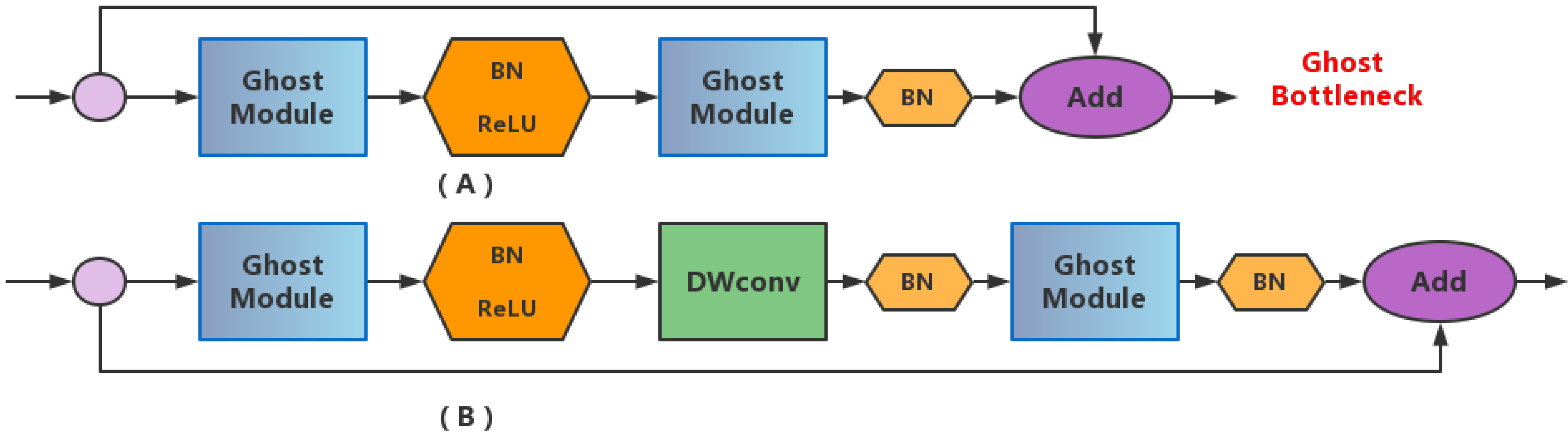
2.6. Lightweight Operation

In the feature maps extracted by deep neural networks, there are partially similar and redundant feature maps, which are called ghost feature maps by Kai Han who is the GhostNet author [38]. The Ghost module is a model compression method that generates a set of feature maps by ordinary convolution and then generates other feature maps by simple linear transformation.

The Ghost bottleneck is stacked by multiple Ghost modules [39], which considerably reduces the computational load while maintaining the accuracy of the model. On this basis, GhostNet mainly consists of a stack of Ghost bottlenecks with the Ghost modules as the building block. In this paper, the enhanced network is handled by the Ghost bottleneck and deep separable convolution, whose specific structure is shown in Figure 4.

2.7. Evaluation Metrics

In terms of the accuracy of the network model, the index of evaluation is precision ratio (P), recall ratio (R), mean Average Precision (mAP), and F1-score.

Precision is used to measure the accuracy of model checking, and Recall is used to assess the comprehensiveness of model detection [40]. Average Precision (AP) is an integration of the Precision over the Recall, and it is indicated as the area of the region surrounded by the curve and the coordinate axis in the P-R plots. The mAP means to take the average of the AP to measure the performance of the whole model [41]. The formulas are shown in (2)–(6).

$$\mathrm{Recall}=\frac{\mathrm{TP}}{\mathrm{TP}+\mathrm{FN}}$$

(2)

$$\mathrm{Precision}=\frac{\mathrm{TP}}{\mathrm{TP}+\mathrm{FP}}$$

(3)

where TP means that jujube in the tested picture were correctly recognized, FP means that other things were misrecognized as jujube, and FN means that jujube was misidentified as other things.

$$\mathrm{AP}={\int }_0^1\mathrm{P}\left(\mathrm{r}\right)\mathrm{dr}$$

(4)

$$\mathrm{mAP}=\frac{{\sum }_{\mathrm{i}=1}^{\mathrm{c}}{\mathrm{AP}}_{\mathrm{i}} }{\mathrm{C}}$$

(5)

where C means the number of categories, i means the serial number.

$$\mathrm{F}1=\frac{2\times \mathrm{Precision}\times \mathrm{Recall}}{\mathrm{Precision}+\mathrm{Recall}}$$

(6)

In terms of the model complexity, it is defined by the number of parameters (weights of the model), the floating point operations (FLOPs), and the overall size of the model:

$$\mathrm{Parameters}=\left[\mathrm{i}\times \left(\mathrm{f}\times \mathrm{f}\right)\times \mathrm{o}\right]+\mathrm{o}$$

(7)

$$\mathrm{FLOPs}=\mathrm{H}\times \mathrm{W}\times \mathrm{Parameters}$$

(8)

where i means the input size, f means the size of the convolutional kernel, o means the output size, and H × W means the size of outputted feature map.

3. Results

3.1. Experiment of Attention Mechanism

This paper used the strategy of multiple combination of four attention mechanism modules to experiment. The same set of parameters was used for each experiment, and the official pre-trained weights of YOLOv5s was used to transfer learning until the model converged. After 50 epochs in the training process, all curves of LOSS reached a relatively stable state. The curve of LOSS was shown in Figure 5, and the conclusion could be seen from the picture: the curve in the early training dropped rapidly, it had leveled off after the 50 epochs and reached convergence, and it had no phenomenon of under-fitting or over-fitting.

In this study, 72 combination schemes were tested by introducing the mixture of different modules to different positions. Finally, a total of 15 schemes of which the mAP reached to 97.6% were selected, and these results are shown in

Table 4. The combination of modules is exponential. This research would present a few of them and draw a figure illustrating the corresponding architecture to explain. “(+)” represents the addition of an attention mechanism to its lower layer, and the unsigned model represents substitution in the current layer.

Model	Precision (%)	Recall (%)	mAP (%)	Max Value of mAP (%)	mAP.5:.95 (%)
YOLOv5s	90.8	88.6	95.7	95.669	80.5
CA	91.7	90.1	96.6	96.59	81.8
ECA	94.2	91	97.3	97.438	87
4SE	93.6	91.2	97.4	97.481	85.8
4ECA	94	91.2	97.6	97.594	86.1
4ECA&CBAM	93.6	91.7	97.6	97.606	86.1
4ECA&CA(+)	91.9	93.2	97.5	97.664	86
4ECA&2SE	93.9	90.9	97.6	97.561	85.9
4ECA&2SE&4CA	93.3	91.8	97.6	97.644	85.9
4CA&CBAM	92.6	92.4	97.6	97.573	85.9
8CA&CBAM	93.9	91.1	97.6	97.601	86
8CA&CBAM(+)	93.2	92.1	97.6	97.608	86.1
8CA&2SE	94	91.3	97.6	97.59	85.9
8CA&2SE(+)	93.8	91.2	97.6	97.561	85.9
7CA&2SE	92.4	92.3	97.6	97.589	86.1
4CA&2SE	92.6	92.9	97.6	97.613	86
4CA&2SE&2TR	94.2	90.9	97.6	97.575	85.5
4CA&CBAM&ECA	93.3	91.9	97.6	97.559	86
4CA&2ECA	92.9	92	97.6	97.569	86.1

.

According to the table, the improvement of network performance by multiple mechanisms of attention was generally better than that of neural network performance by a single attention. The improved network converged after 43,350 iterations, and each index increased in different degrees. To screen a model of the highest accuracy by comparing the F1 and the mAP.5,.95: in three schemes where the F1-score reached 0.93 based on a confidence above 0.610, including ECA + 2SE + 4CA, 4CA + 2SE + 2TR and 4CA + 2ECA, and the mAP.5:.95 of 4CA + 2ECA was the highest one at different thresholds. Therefore, this scheme of 4CA + 2ECA which had the best result was named as YOLOv5-CE, and the mAP of this model was compared with different versions under the YOLOv5 network. The results are shown in Figure 6.

3.2. Optimization Experiment of the C3 Module

The experiment was divided into three improved schemes of (2,3,6,2), (2,4,6,2), and (2,6,6,2). It can be obtained from the above experiments that the parameters, FLOPs, speed of inference, and the 4ECA model size were the most similar to the original network on the basis of the mAP reaching 97.6%. Accordingly, the improved network of YOLOv5_4ECA was trained as the baseline network to test the optimization effect of the C3 module. The results are shown in Figure 7.

As available from the above figure, when the number of C3 modules in layers 2, 4, 6, and 8 of the backbone network is reduced from (×3, ×6, ×9, ×3) to (×2, ×6, ×6, ×2), the accuracy indexes (mAP and mAP.5:.95) remain basically unchanged. Meanwhile, there is a slight decrease in the complexity index, where the parameters decreased by 2.3%, so this scheme had the best effect among three schemes.

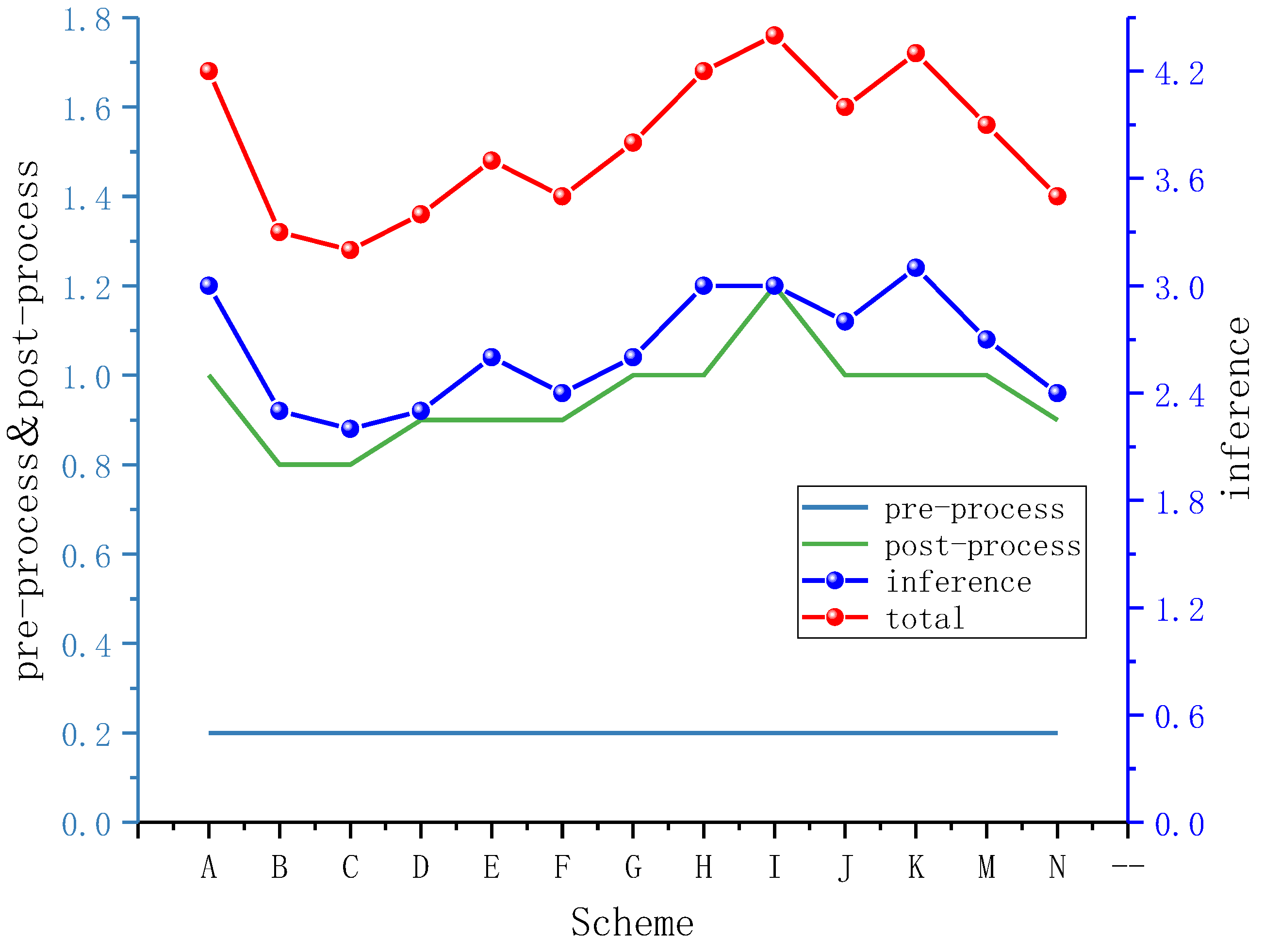
3.3. Performance Analysis of Different Lightweight Schemes

To choose the best lightweight scheme, this paper introduced the Ghost modules and the Deep Separable Convolution to different locations in the baseline network. The specific results are shown in

Table 5. Results of the lightweight experiment. “_neck” means that the location of the introduction is the neck network, “_all” means that the location of the introduction is the full network, and the unmarked means that the location of the introduction is the backbone network.

Location	Precision (%)	Recall (%)	mAP (%)	mAP.5:.95 (%)	Parameters	Floating-Point Operations per Second (G)	Inference Time (ms)	Model Size (MB)
4ECA	94	91.2	97.6	86.1	7,015,540	15.8	3.0	14.4
Ghost	93.4	91.2	97.4	84.5	5,853,052	12.4	3.0	12.1
Ghost_neck	94	90.8	97.4	85.7	6,053,252	13.9	3.1	12.5
Ghost_all	92.8	91.5	97.3	84.2	4,899,580	10.5	2.7	10.2
DWconv	94.3	90.5	97.4	85	5,457,460	12.1	2.5	11.2
DWconv_neck	94.2	90.8	97.4	85.7	6,118,644	14.7	3.0	12.5
DWconv_all	93.4	91.3	97.4	84.7	4,560,564	11	2.3	9.5
Ghost&DWconv_all	91.8	91.4	97	82.9	3,398,076	7.6	2.1	7.5
Ghost_neck&DWconv_all	93.2	91.4	97.4	84.5	3,598,276	9	2.3	7.6
Ghost_all&DWconv_all	92.8	90.1	97	82.1	2,435,778	5.6	2.1	5.5
Ghost&DWconv	93.3	90.6	97.1	82.8	4,294,972	8.7	2.4	9.1
(Ghost&DWconv)_neck	93	91.9	97.4	85.4	5,156,356	12.7	2.9	10.7
Ghost_neck&DWconv	93.6	90.6	97.3	84.7	4,495,172	10.1	2.5	9.4
Ghost&DWconv_neck	92.6	91.7	97.3	84.3	4,956,156	11.3	2.7	10.3

.

From the above table, we see that the best scheme consists of introducing the Ghost module in the neck and replacing the ordinary convolutional layers with depthwise separable convolution. To ensure the validity of the lightweight, 15 schemes with a 97.6% mAP in Table 4 were selected for lightweight manipulation in this paper (Section 3.1). The results are shown in

Table 6. The comparison of a lightweight improved network and an original network.

Lightweight Network	mAP (%)	mAP.5:.95 (%)	Parameters	FLOPs (B)	Detection Time (ms)				Model Size (MB)
					Pre-Process	Inference	Post-Process	Total
YOLOv5s	95.7	80.5	7,015,519	15.8	0.2	3.0	1.0	4.2	14.4
4ECA	97.4	84.5	3,598,276	9	0.2	2.3	0.8	3.3	7.7
ECA & SE	97.4	84.4	3,631,044	9	0.2	2.2	0.8	3.2	7.8
4ECA & SE	97.3	84.1	3,466,945	8.5	0.2	2.3	0.9	3.4	7.0
4ECA & CA	97.3	84.4	3,623,924	8.6	0.2	2.6	0.9	3.7	7.8
4ECA&CBAM	97.3	84.1	4,812,326	9.1	0.2	2.4	0.9	3.5	10.1
4ECA & 2SE & 4CA	97.2	84.1	3,706,172	8.1	0.2	2.6	1.0	3.8	8.1
8CA & CBAM	97.3	84.1	3,751,521	8.1	0.2	3.0	1.0	4.2	8.1
8CA & 2SE(+)	97.3	84.2	3,784,191	8.2	0.2	3.0	1.2	4.4	8.1
4CA&2SE(+)	97.4	84.2	3,741,831	8.1	0.2	2.8	1.0	4.0	8.1
4CA & 2SE & 2TR	97.3	83.9	3,333,031	7.2	0.2	3.1	1.0	4.3	7.2
4CA & CBAM & 3ECA	97.3	84.1	3,709,170	7.6	0.2	2.7	1.0	3.9	7.9
4CA & 2ECA	97.3	84.2	2,495,117	6.1	0.2	2.4	0.9	3.5	5.4

.

As shown in the table above, after lightening the YOLOv5-CE network compared to the original YOLOv5s network, mAP increased by 1.6%, and parameters and FLOPs decreased by 64.43% and 61.49%, respectively. Meanwhile, the model size and the detection time decreased to 37.5% and 83.3%, respectively. The specific changes in the detection time are shown in Figure 8.

The detection time is the average detection time per image in the validation set (contains 1250 images), including the pre-processing, inference, and post-processing steps. It can be seen from Figure 8 that the pre-processing time curve is constant, and the post-processing time curve generates small amplitude fluctuations due to the optimization of the loss function. Therefore, the detection time changes mainly by the inference time. There are two main reasons for the reduction of the detection time and the parameters. On the one hand, the simple linear transformation of the Ghost module is faster than the ordinary convolution operation. The amount of computation of the Ghost module is approximately reduced by s (the number of ghost feature maps) times compared with the ordinary convolution module. On the other hand, the Deep Separable Convolution replaces the big convolution kernel with the relatively small convolution kernel. In terms of inference, the decrease in computation of convolution operations leads to a shorter model detection time.

It is demonstrated that this scheme not only maintained the accuracy of network, but also reduced the parameters, FLOPs, and detection time. Accordingly, this scheme which had the best lightweight effect is named YOLOv5-GCE, and its structure is shown in

Table 7. The YOLOv5 lightweight network structure. The input “−1” in the table represents the input from the previous layer. The tensor information includes the number of input channels of the module, output channels, convolution kernel size, step length, and grouping.

Number	Input	Parameters	Module	Tensor Information	Number	Input	Parameters	Module	Tensor Information
0	−1	3520	Conv	(3, 32, 6, 2, 2)	15	−1	1024	DWconv	(512, 256, 1, 1)
1	−1	704	DWconv	(32, 64, 3, 2)	16	−1	0	Upsample	(None, 2, ’nearest’)
2	−1	18,816	C3	(64, 64, 1)	17	(−1, 7)	0	Concat	(1)
3	−1	1408	DWconv	(64, 128, 3, 2)	18	−1	208,608	Ghost	(512, 256, 1, Fasle)
4	−1	115,712	C3	(128, 128, 2)	19	−1	512	DWconv	(256, 128, 1, 1)
5	−1	6704	CA	(128, 128, 32)	20	−1	0	Upsample	(None, 2, ’nearest ’)
6	−1	2816	DWconv	(128, 256, 3, 2)	21	(−1, 4)	0	Concat	(1)
7	−1	625,152	C3	(256, 256, 3)	22	−1	53,104	Ghost	(256, 128, 1, Fasle)
8	−1	20,040	CA	(256, 256, 32)	23	−1	1408	DWConv	(128, 128, 3, 2)
9	−1	5632	DWconv	(256, 512, 3, 2)	24	(−1, 19)	0	Concat	(1)
10	−1	3	ECA	(512)	25	−1	143,072	Ghost	(256, 256, 1, Fasle)
11	−1	25,648	CA	(512, 512, 32)	26	−1	2816	DWconv	(256, 256, 3, 2)
12	−1	656,896	SPPF	(512, 512, 5)	27	(−1, 15)	0	Concat	(1)
13	−1	3	ECA	(512)	28	−1	564,672	Ghost	(512, 512, 1, Fasle)
14	−1	25,648	CA	(512, 512, 32)	29	(22, 25, 28)	18,879	Detect	/

.

The P-R curves of the improved network and its lightweight network are shown in Figure 9. The mAP of mature fruit is 98.1%, while the mAP of immature fruit decreases from 97.2% to 96.8%. As a result, the mAP of the overall network decreased from 97.7% to 97.4%. This is because the color of the immature fruit is similar to the background containing the leaves and the crown, and thus the ability of the lightweight networks that extract features from small targets in this background was subsequently weakened.

3.4. Ablation Experiment

The ablation study is to see the effects on performance by removing some features of the detection algorithm. In order to verify the effect of every improved point for the network performance, this paper selected six improved methods and the original YOLOv5s network to perform the ablation experiment.

YOLOv5 had a mechanism of Early Stopping which automatically stopped training when mAP was not increased within 100 consecutive experiments. When the epoch was set to 300, it automatically stopped training at approximately the 260th epoch. This means that the experiment reached complete convergence and mAP was no longer increased, when the model training reached about the 160th epoch. In order to ensure the effectiveness of the model, the training results after the 200th epoch were selected. The whole training process of the improved network is shown in Figure 10.

The results of the ablation experiment are shown in

Table 8. Improved network ablation experiments. “√” represents that the improved method is applied in the model. “×” means that the improved method is not used in the model.

Model	Data Balance	C3	Attention	Loss Function	Multi-Scale	Lightweight	mAP (%)	mAP.5:.95 (%)	Parameters	FLOPs (G)	Model Size (MB)
YOLOv5s	×	×	×	×	×	×	87.8	74.7	7,015,540	15.8	14.4
Improvement 1	√	×	×	×	×	×	95.7	80.5	7,015,519	15.8	14.4
Improvement 2	√	√	×	×	×	×	95.7	81.9	6,851,441	15.3	13.8
Improvement 3	√	√	√	×	×	×	97.6	85.9	5,942,252	12.5	12.2
Improvement 4	√	√	√	√	×	×	97.7	89.5	5,942,252	12.5	12.2
Multi-scale	√	√	√	√	√	×	97.7	89.5	5,942,252	15.2	12.2
Improvement 5	√	√	√	√	×	√	97.4	84.2	2,495,117	6.1	5.4

. The first improvement is the balance of data, the second improvement is optimization of the C3 module, the third improvement is the mixed introduction of multiple mechanisms of attention, the fourth improvement is optimization of the loss function, and the fifth improvement is the lightweight operation.

From the above table, the mAP increased by 7.9% after using the balanced datasets, which contained 12,502 images, taken as the raw data. After the optimization of the C3 module, the decline of the parameters and FLOPs were small, and the accuracy index (mAP and mAP.5:.95) remained basically unchanged. Based on this improvement, the mAP increased by 1.9% and the rest of the indicators of the accuracy increased by introducing the hybrid attention mechanisms. Meanwhile, the parameters, FLOPs, and model size reduced to 84.7%, 79.11%, and 84.72% of the original YOLOv5s network. Then, it was demonstrated that the optimization of loss function and the multi-scale training had less of an effect on the accuracy of the model, while it was found to reduce the occurrence of false detection and missed detection by the comparison of the detection effect of the pictures. Finally, in the lightweight experiment, the mAP and mAP (.5,.95) increased by 1.7% and 3.7% compared with the original YOLOv5s network, and the parameters, FLOPs, and model size reduced to 35.57%, 38.61%, and 37.50% of the original YOLOv5s network, respectively.

In order to show the recognition effect of the improved algorithm to the field flat jujube, the pictures with different obstacles, different light conditions, and different backgrounds were selected for detection and comparison. The results are shown in Figure 11.

3.5. Comparison Experiments with Different Networks

Currently, the most commonly used YOLO target detection algorithms contain YOLOv3, YOLOv4, YOLOv5, and YOLOx. The VGG-16 and Darknet-19 network as the backbone network of YOLOv1 and YOLOv2 [42], respectively, and the YOLOv3 [43] takes advantage of the Darknet-53 backbone network which relies on 53 convolutional layers to improve the ability of feature extraction. YOLOv4 [44] uses the CSPDarknet53 as the backbone network, and it adds the mosaic and cut-mix data augmentation methods in the input; and, the SPP module and the PAN structure are added in the neck network. On the basis of the four structures (s, m, l, and x) of the YOLOv5, YOLOx [45] uses the mosaic and the mix-up data augmentation methods in the input, and it replaces the YOLO head with the decoupled head. These algorithms have a different dimension, average accuracy, speed of detection, and training.

In order to validate the effectiveness of improvement, the mainstream YOLO target detection algorithms (v3, v4, v5n, v5s_5.0, v5s_6.0, and x-s) and the improved algorithms (YOLOv5s-CE and YOLOv5-GCE) were selected for the experiments of comparison, and the results are shown in

Table 9. Comparison results of the mainstream YOLO target detection algorithms and improved algorithms.

Model	Precision (%)	Recall (%)	mAP (%)	Parameters	FLOPs (G)	Model Size (MB)
YOLOv3	87.6	87.5	90.7	61,631,434	116.3	234.6
YOLOv4	86	89.1	91.7	63,953,841	127.2	244.3
YOLOx-s	90	90.9	96.3	13,714,753	26.8	34.3
YOLOv5s-5.0	90.6	87.4	95.1	7,056,607	16.3	14.5
YOLOv5s-6.0	90.8	88.6	95.7	7,015,519	15.8	14.4
YOLOv5-CE	92.9	92	97.7	5,942,252	12.5	12.2
YOLOv5-GCE	94	90	97.4	2,495,117	6.1	5.4
YOLOv5n	62.4	74.1	73.9	1,761,871	4.2	3.8

.

From the above table, all the indicators of YOLOv5s_6.0 were better than that of YOLOv5s_5.0, and although the model size of YOLOv5n was 26.39% of the original YOLOv5s_6.0 network, the accuracy also decreased significantly. In order to show the detection effect of these algorithms visually, we plotted them in Figure 12.

As can be seen from Figure 12, the detection accuracy of the improved algorithm (YOLOv5-CE) is higher than the other seven algorithms. The YOLOv5-GCE network has a more obvious advantage in accuracy and complexity than YOLOv3, YOLOv4, and YOLOx-s. Meanwhile, its parameters and model size decreased to 35.57% and 44.26% of the YOLOv5-CE, respectively, and the model size was compressed to 5.4 MB.

4. Discussion

Deep learning combined with transfer learning are used to detect the field flat jujube in this paper. The major improvements include structural improvements, the introduction of attention mechanisms, the optimization of loss function, and lightweight operations. Although the mAP of the improved network reaches 97.7% and it has a good effect on recognition of the flat jujube in a natural environment, increasing rate recognition and accuracy. There is still the phenomena of false and missed detection. Additionally, there are still some areas for improvement in this document.

In terms of computer vision on fruit detection and classification, Ibrahim et al. [46] used the fruit images for 52 species belonging to four different families to build a deep learning analysis dataset, and they put forward a novel Convolution Neural Network (CNN) model architecture to extract the fruit features. Compared with the above paper, our proposed architecture is relatively simple, and subsequent studies should attempt to apply the proposed algorithm to other objects to enhance the generalization of the model.

In order to obtain a better effect of training, a larger dataset is needed to take full advantage of deep learning. In the stage of data acquisition, we should consider the effects of other conditions (such as uneven illumination, recognition at night, greasy weather, overexposure). To get high-resolution pictures, the Single Lens Reflex (SLR) camera with the function of auto focus high pixels is used in the process of collecting data. As a result, there is a blurry background and the replacement of front and rear scene in some pictures. These problematic pictures will affect the identification effect and even contribute to the rate of missed and false detections. Therefore, the loss by the function of auto focus should be taken into account, and we should use cameras that turn off the function of auto focus to shoot to ensure the quality of pictures. Future studies should rely on a variety of lightweight networks (such as MobileNet, EfficientNet, ShuffleNet, and GhostNet, etc.) while maintaining model stability and accuracy to achieve real-time recognition of the flat jujube.

5. Conclusions

In view of the problem of low efficiency of accurate identification for flat jujube in the natural environment, this paper proposes a target detection algorithm based on improved YOLOv5. In terms of the improvement of accuracy, two attention mechanisms (CA, ECA) are introduced to improve network performance. In terms of the reduction of complexity, this research makes lightweight operation on the model by improving structure and the number of the C3 modules, and introducing the Ghost module and the Depthwise Separable Convolution. With regard to the optimization of the learning process, we proposed multi-scale training. Meanwhile, the loss function and the post-processing are optimized accordingly. The following conclusions can be drawn from our experiments:

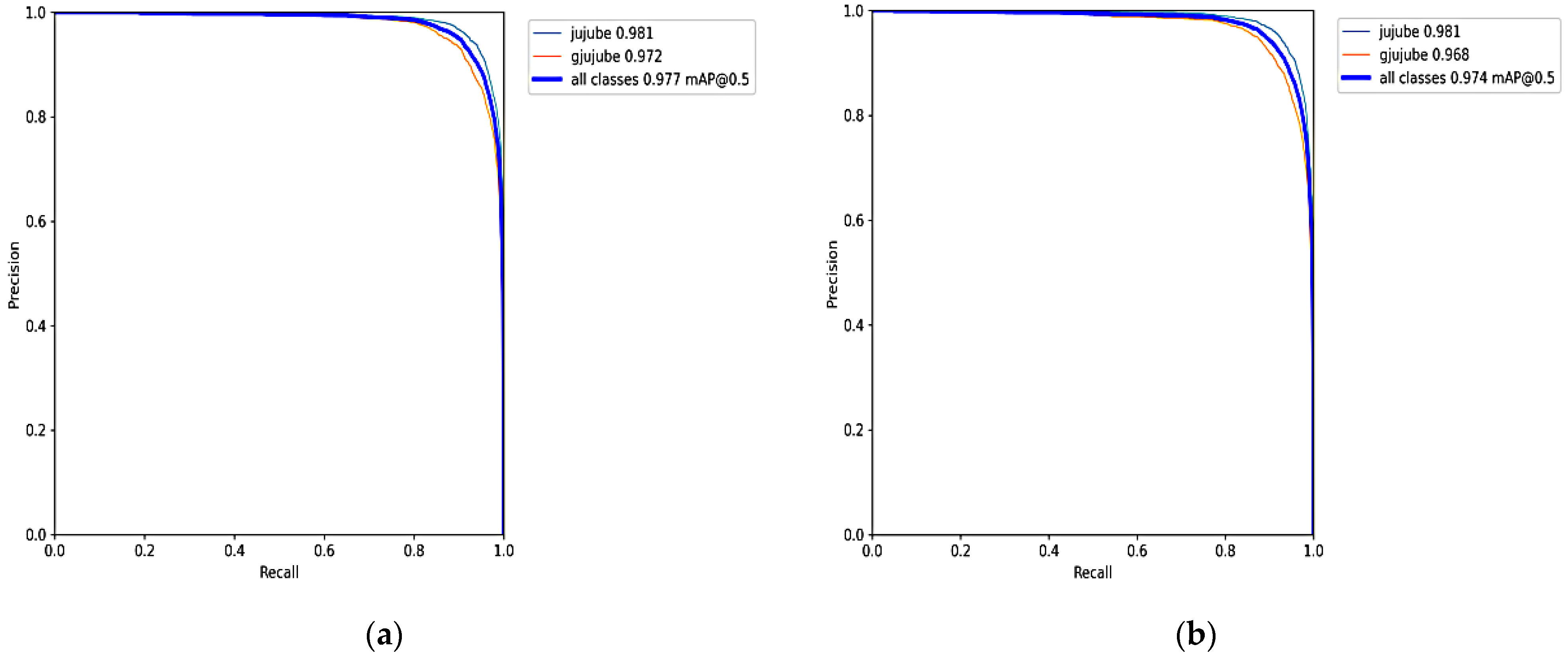
• Through the mixed introduction of multiple attention, the AP of mature and immature jujube reaches 98.1% and 97.2%, respectively. The mAP of the YOLOv5-CE network reaches 97.7%; it increases by 2% compared with the original YOLOv5s network.
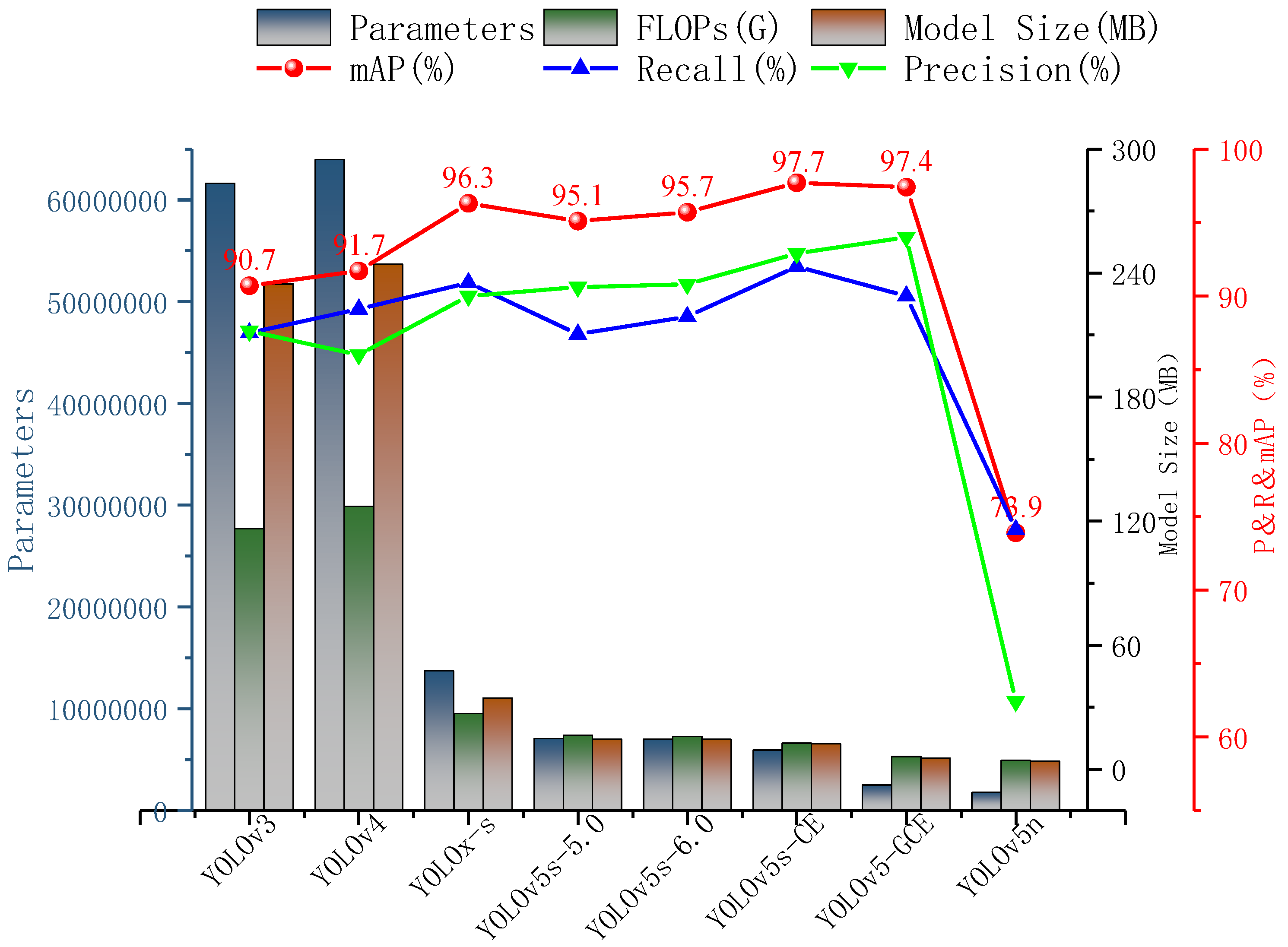
• After the lightweight operation on the improved network, the mAP reaches 97.4%; it increases by 1.7% compared with the original YOLOv5s network. In terms of the complexity of the model, the parameters and the FLOPs decrease by 64.43% and 61.39%, the detection time and the model size are compressed to 3.5 ms and 5.4 MB, respectively.
• Compared with the original YOLOv5s, YOLOv5n, YOLOx-s, YOLOv4, and YOLOv3 model, the mAP of YOLOv5-GCE increases by 1.7%, 23.5%, 9%, 5.7%, and 6.7%, respectively. Additionally, the model size of YOLOv5-GCE reaches 5.4 MB, which is slightly larger than YOLOv5n (3.8 MB), but it is compressed by 62.5%, 84.3%, 97.8%, and 97.7% compared with the rest of the models, respectively.

This research uses the method of deep learning to identify the flat jujube in the natural environment for the first time. Through the improvement and the lightweight operation on the YOLOv5 network, it realizes real-time detection of high precision on the field flat jujube, and it reduces the rate of false identifications for field flat jujube in a near-color background containing leaves and crown. The proposed algorithm has a greater advantage in performance, meeting the requirement of accuracy and immediacy for picking robots. Moreover, it is conducive to the lightweight deployment of the model in subsequent hardware devices, particularly those asking for real-time detection of the flat jujube field mounted on mobile terminals.

References

1. Kateb, F.A.; Monowar, M.M.; Hamid, A.; Ohi, A.Q.; Mridha, M.F. FruitDet: Attentive Feature Aggregation for Real-Time Fruit Detection in Orchards. Agronomy 2021, 11, 2440. [Google Scholar] [CrossRef]
2. Zhang, W.; Wang, J.; Liu, Y.; Chen, K.; Li, H.; Duan, Y.; Wu, W.; Shi, Y.; Guo, W. Deep-learning-based in-field citrus fruit detection and tracking. Hortic. Res. 2022, 9, 6526907. [Google Scholar] [CrossRef] [PubMed]
3. Sozzi, M.; Cantalamessa, S.; Cogato, A.; Kayad, A.; Marinello, F. Automatic Bunch Detection in White Grape Varieties Using YOLOv3, YOLOv4, and YOLOv5 Deep Learning Algorithms. Agronomy 2022, 12, 319. [Google Scholar] [CrossRef]
4. Tassis, L.M.; de Souza, J.E.T.; Krohling, R.A. A deep learning approach combining instance and semantic segmentation to identify diseases and pests of coffee leaves from in-field images. Comput. Electron. Agric. 2021, 186, 106191. [Google Scholar] [CrossRef]
5. Math, R.M.; Dharwadkar, N.V. Early detection and identification of grape diseases using convolutional neural networks. J. Plant Dis. Prot. 2022, in press. [Google Scholar] [CrossRef]
6. Fan, X.; Xu, Y.; Zhou, J.; Li, Z.; Peng, X.; Wang, X. Detection system for grape leaf diseases based on transfer learning and updated CNN. Trans. Chin. Soc. Agric. Eng. (Trans. CSAE) 2021, 37, 151–159. [Google Scholar] [CrossRef]
7. Wang, X.; Tang, J.; Whitty, M. Data-centric analysis of on-tree fruit detection: Experiments with deep learning. Comput. Electron. Agric. 2022, 194, 106748. [Google Scholar] [CrossRef]
8. Kimutai, G.; Ngenzi, A.; Said, R.N.; Kiprop, A.; Förster, A. An Optimum Tea Fermentation Detection Model Based on Deep Convolutional Neural Networks. Data 2020, 5, 44. [Google Scholar] [CrossRef]
9. Janarthan, S.; Thuseethan, S.; Rajasegarar, S.; Lyu, Q.; Zheng, Y.; Yearwood, J. Deep Metric Learning Based Citrus Disease Classification With Sparse Data. IEEE Access 2020, 8, 162588–162600. [Google Scholar] [CrossRef]
10. Luo, Y.; Wei, Y.; Lin, L.; Lin, F.; Su, F.; Sun, W. Origin discrimination of Fujian white tea using gas chromatography-ion mobility spectrometry. Trans. Chin. Soc. Agric. Eng. (Trans. CSAE) 2021, 37, 264–273. [Google Scholar] [CrossRef]
11. Caladcad, J.A.; Cabahug, S.; Catamco, M.R.; Villaceran, P.E.; Cosgafa, L.; Cabizares, K.N.; Hermosilla, M.; Piedad, E.J. Determining Philippine coconut maturity level using machine learning algorithms based on acoustic signal. Comput. Electron. Agric. 2020, 172, 105327. [Google Scholar] [CrossRef]
12. Turkoglu, M.; Hanbay, D.; Sengur, A. Multi-model LSTM-based convolutional neural networks for detection of apple diseases and pests. J. Ambient Intell. Humaniz. Comput. 2019, 1–11. [Google Scholar] [CrossRef]
13. Ren, R.; Zhang, S.; Sun, H.; Gao, T. Research on Pepper External Quality Detection Based on Transfer Learning Integrated with Convolutional Neural Network. Sensors 2021, 21, 5305. [Google Scholar] [CrossRef] [PubMed]
14. Hussain, D.; Hussain, I.; Ismail, M.; Alabrah, A.; Ullah, S.S.; Alaghbari, H.M. A Simple and Efficient Deep Learning-Based Framework for Automatic Fruit Recognition. Comput. Intell. Neurosci. 2022, 2022, 6538117. [Google Scholar] [CrossRef]
15. Ukwuoma, C.C.; Zhiguang, Q.; Bin Heyat, B.; Ali, L.; Almaspoor, Z.; Monday, H.N. Recent Advancements in Fruit Detection and Classification Using Deep Learning Techniques. Math. Probl. Eng. 2022, 2022, 9210947. [Google Scholar] [CrossRef]
16. Shahi, T.B.; Sitaula, C.; Neupane, A.; Guo, W. Fruit classification using attention-based MobileNetV2 for industrial applications. PLoS ONE 2022, 17, e0264586. [Google Scholar] [CrossRef]
17. Khudayberdiev, O.; Zhang, J.; Abdullahi, S.M.; Zhang, S. Light-FireNet: An efficient lightweight network for fire detection in diverse environments. Multimedia Tools Appl. 2022, 1–20. [Google Scholar] [CrossRef]
18. Park, C.; Lee, S.; Han, H. Efficient Shot Detector: Lightweight Network Based on Deep Learning Using Feature Pyramid. Appl. Sci. 2021, 11, 8692. [Google Scholar] [CrossRef]
19. Zheng, T.; Jiang, M.; Feng, M. Vision based target recognition and location for picking robot. Instrum. J. Available online: https://kns.cnki.net/kcms/detail/detail.aspx?doi=10.19650/j.cnki.cjsi.J2107650 (accessed on 13 April 2022). [CrossRef]
20. Akshatha, K.R.; Karunakar, A.K.; Shenoy, S.B.; Pai, A.K.; Nagaraj, N.H.; Rohatgi, S.S. Human Detection in Aerial Thermal Images Using Faster R-CNN and SSD Algorithms. Electronics 2022, 11, 1151. [Google Scholar] [CrossRef]
21. Gu, Y.; Wang, S.; Yan, Y.; Tang, S.; Zhao, S. Identification and Analysis of Emergency Behavior of Cage-Reared Laying Ducks Based on YoloV5. Agriculture 2022, 12, 485. [Google Scholar] [CrossRef]
22. Zhang, X.; Gao, Q.; Pan, D.; Zhang, W. Picking recognition research of pineapple in complex field environment based on improved YOLOv3. J. Chin. Agric. Mech. 2021, 42, 201–206. [Google Scholar] [CrossRef]
23. Zhang, H.; Fu, Z.; Han, W.; Yang, G.; Niu, D.; Zhou, X. Detection Method of Maize Seedlings Number Based on Improved YOLO. J. Agric. Mach. 2021, 52, 221–229. [Google Scholar] [CrossRef]
24. Hnewa, M.; Hayder, R. Integrated Multiscale Domain Adaptive YOLO. arXiv 2022, arXiv:2202.03527. [Google Scholar]
25. Kim, N.; Kim, J.-H.; Won, C.S. FAFD: Fast and Accurate Face Detector. Electronics 2022, 11, 875. [Google Scholar] [CrossRef]
26. Gonzales-Martinez, R.; Machacuay, J.; Rotta, P.; Chinguel, C. Hyperparameters Tuning of Faster R-CNN Deep Learning Transfer for Persistent Object Detection in Radar Images. IEEE Lat. Am. Trans. 2022, 20, 677–685. [Google Scholar] [CrossRef]
27. Hooda, M.; Rana, C.; Dahiya, O.; Shet, J.P.; Singh, B.K. Integrating LA and EDM for Improving Students Success in Higher Education Using FCN Algorithm. Math. Probl. Eng. 2022, 2022, 7690103. [Google Scholar] [CrossRef]
28. Kavitha, T.S.; Prasad, K.S. A novel method of compressive sensing MRI reconstruction based on sandpiper optimization algorithm (SPO) and mask region based convolution neural network (mask RCNN). Multimedia Tools Appl. 2022, 1–24. [Google Scholar] [CrossRef]
29. Ortenzi, L.; Figorilli, S.; Costa, C.; Pallottino, F.; Violino, S.; Pagano, M.; Imperi, G.; Manganiello, R.; Lanza, B.; Antonucci, F. A Machine Vision Rapid Method to Determine the Ripeness Degree of Olive Lots. Sensors 2021, 21, 2940. [Google Scholar] [CrossRef]
30. Faisal, M.; Albogamy, F.; Elgibreen, H.; Algabri, M.; Alqershi, F.A. Deep Learning and Computer Vision for Estimating Date Fruits Type, Maturity Level, and Weight. IEEE Access 2020, 8, 206770–206782. [Google Scholar] [CrossRef]
31. Redmon, J.; Divvala, S.; Girshick, R.; Farhadi, A. You Only Look Once: Unified, Real-Time Object Detection. In Proceedings of the IEEE Conference on Computer Vision and Pattern Recognition (CVPR), Las Vegas, NV, USA, 26 June–1 July 2016; Available online: https://arxiv.org/abs/1506.02640 (accessed on 13 April 2022).
32. Zheng, J.; Sun, S.; Zhao, S. Fast ship detection based on lightweight YOLOv5 network. IET Image Process. 2022, 16, 1585–1593. [Google Scholar] [CrossRef]
33. Park, S.-S.; Tran, V.-T.; Lee, D.-E. Application of Various YOLO Models for Computer Vision-Based Real-Time Pothole Detection. Appl. Sci. 2021, 11, 11229. [Google Scholar] [CrossRef]
34. Sharma, T.; Debaque, B.; Duclos, N.; Chehri, A.; Kinder, B.; Fortier, P. Deep Learning-Based Object Detection and Scene Perception under Bad Weather Conditions. Electronics 2022, 11, 563. [Google Scholar] [CrossRef]
35. Hou, Q.; Zhou, D.; Feng, J. Coordinate attention for efficient mobile network design. In Proceedings of the IEEE/CVF Conference on Computer Vision and Pattern Recognition, Nashville, TN, USA, 20–25 June 2021; pp. 13713–13722. [Google Scholar]
36. Wang, J.; Sun, Z.; Guo, P.; Zhang, L. Improved leukocyte detection algorithm of YOLOV5. Comput. Eng. Appl. 2022, 58, 134–142. [Google Scholar] [CrossRef]
37. Chaudhari, S.; Mithal, V.; Polatkan, G.; Ramanath, R. An Attentive Survey of Attention Models. ACM Trans. Intell. Syst. Technol. 2021, 12, 1–32. [Google Scholar] [CrossRef]
38. Han, K.; Wang, Y.; Tian, Q.; Guo, J.; Xu, C.; Xu, C. Ghostnet: More features from cheap operations. In Proceedings of the IEEE/CVF Conference on Computer Vision and Pattern Recognition, Seattle, WA, USA, 13–19 June 2020. [Google Scholar]
39. Sandler, M.; Howard, A.; Zhu, M.; Zhmoginov, A.; Chen, L.-C. MobileNetV2: Inverted residuals and linear bottlenecks. In Proceedings of the 2018 International Conferenceon Computer Visionand Pattern Recognition, Salt Lake City, UT, USA, 18–23 June 2018; IEEE: Piscataway, NJ, USA, 2018; pp. 4510–4520. [Google Scholar] [CrossRef] [Green Version]
40. Hsu, W.-Y.; Lin, W.-Y. Adaptive Fusion of Multi-Scale YOLO for Pedestrian Detection. IEEE Access 2021, 9, 110063–110073. [Google Scholar] [CrossRef]
41. Liu, Y.; Lu, B.; Peng, J.; Zhang, Z. Research on the use of YOLOv5 object detection algorithm in mask wearing recognition. World Sci. Res. J. 2020, 6, 276–284. [Google Scholar]
42. Redmon, J.; Farhadi, A. YOLO9000: Better, faster, stronger. In Proceedings of the IEEE Conference on Computer Vision and Pattern Recognition, Honolulu, HI, USA, 21–26 July 2017. [Google Scholar]
43. Redmon, J.; Farhadi, A. Yolov3: An incremental improvement. arXiv 2018, arXiv:1804.02767. [Google Scholar]
44. Bochkovskiy, A.; Wang, C.-Y.; Liao, H.-Y.M. Yolov4: Optimal speed and accuracy of object detection. arXiv 2020, arXiv:2004.10934. [Google Scholar]
45. Ge, Z.; Liu, S.; Wang, F.; Li, Z.; Sun, J. Yolox: Exceeding yolo series in 2021. arXiv 2021, arXiv:2107.08430. [Google Scholar]
46. Ibrahim, N.M.; Gabr, D.G.I.; Rahman, A.-U.; Dash, S.; Nayyar, A. A deep learning approach to intelligent fruit identification and family classification. Multimed. Tools Appl. 2022, 1–16. [Google Scholar] [CrossRef]
Figure 1. Data samples under different environments. (A) occluded by branches (B) occluded by leaves (C) overlap (D) sky background (E) soil background (F) crown background (G) sunlight angle (H) sidelight angle (I) backlight angle.
Agriculture 12 00717 g001
Figure 2. The structure of improved C3 module and ECA (Efficient Channel Attention) module. C, H, and W refer to the channels, height, and width of the input image. Conv means that the convolutional layer (A) The red dotted box indicates that the convolution layer has been removed. The blue dotted box indicates that the convolutional layer (Kernel size: 1 × 1), BN (Batch Normalization) layer, and SiLU (Sigmoid Weighted Liner Unit) activation function together form the CBS (Convolutional layer, Batch Normalization, Sigmoid Weighted Liner Unit) module. (B) GAP indicates that Global Average Pooling. “⊗” indicates that element-wise product. The purple dotted box indicates that the fast 1D convolution to replace FC (Full Connection) layers in channel attention module.
Agriculture 12 00717 g002
Figure 3. Structure of loss function. (a) GIOU (Generalized Intersection over Union): A and B indicate that the boxes of true and predicted, the red dotted box indicates the special position of A and B, the green area means the required intersection area. (b) C indicates the diagonal distance from the minimum circumscribed rectangle bounding A and B. d indicates that the Euclidean distance between the center points of the boundary box A and B.
Agriculture 12 00717 g003
Figure 4. The structure diagram of Ghost Bottleneck. BN means that Batch Normalization layer. Add operation means that the superposition of information. ReLU means that the Rectified Linear Unit. (A) Stride = 1 (B) Stride = 2. DWconv means that the depthwise separable convolution.
Agriculture 12 00717 g004
Figure 5. Convergence of the loss functions of training and validation sets. (A) Training loss (B) Validation loss.
Agriculture 12 00717 g005
Figure 6. The accuracy comparative results of the YOLOv5n, YOLOv5s, YOLOv5m and YOLOv5s-CE at different IoU thresholds. (A) mAP (mean Average Precision) : IOU = 0.5 (B) mAP.5:.95 : IOU = 0.5~0.95 (stride = 0.05).
Agriculture 12 00717 g006
Figure 7. The Optimization of the C3 module. Content within the “()” represents the number of C3 modules in the backbone network.
Agriculture 12 00717 g007
Figure 8. The detection time curves under different schemes. “A–N” represents the different schemes presented in Table 6.
Agriculture 12 00717 g008
Figure 9. PR_curve of the YOLOv5s-CE and YOLOv5-GCE (a) Improved network; (b) Lightweight Improved network.
Agriculture 12 00717 g009
Figure 10. The complete training process of YOLOv5-GCE network.
Agriculture 12 00717 g010
Figure 11. Identification effect of different algorithms under the different environments. (A,C,E) represent the identification effect of YOLOv5s algorithm. (B,D,F) represent the identification effect of YOLOv5-GCE algorithm. The different environments contain obstacle (branches, leaves, and jujube), background (soil, sky, and crown), and light (sunlight, sidelight, and backlight). The green and the blue dotted boxes indicate the missed and false detections, respectively.
Agriculture 12 00717 g011
Figure 12. Comparison results in terms of accuracy (P, R, and mAP) and complexity (Parameters, FLOPs, and Model Size) of detection algorithms.
Agriculture 12 00717 g012