Article

Interaction Simulation of Vadose Zone Water and Groundwater in Cele Oasis: Assessment of the Impact of Agricultural Intensification, Northwestern China

1
State Key Laboratory of Desert and Oasis Ecology, Xinjiang Institute of Ecology and Geography, Chinese Academy of Sciences, Urumqi 830011, China
2
Cele National Station of Observation and Research for Desert Grassland Ecosystem in Xinjiang, Cele 848300, China
3
University of Chinese Academy of Sciences, Beijing 100049, China
4
State Key Laboratory of Biogeology and Environmental Geology, China University of Geosciences, Wuhan 430000, China
*
Author to whom correspondence should be addressed.
Agriculture 2022, 12(5), 641; https://doi.org/10.3390/agriculture12050641
Submission received: 20 March 2022 / Revised: 23 April 2022 / Accepted: 27 April 2022 / Published: 28 April 2022
(This article belongs to the Special Issue Precision Water Management in Dryland Agriculture)

Abstract

:
Agricultural intensification has boosted land productivity, but it has also created new sustainability issues. As one of the most important human habitations and agricultural farming areas in arid areas, the Cele Oasis has a very developed agricultural system. This paper studies the long-term effects of different types of agricultural intensification strategies on groundwater level fluctuations in the Cele Oasis. A soil water flow (HYDRUS-1D) and aquifer simulation (MODFLOW) coupling model were used to construct the geometric structures of the vadose zone and saturated zone in the Cele Oasis and to analyze the recharge and discharge mechanism of the oasis. The results showed that HYDRUS-1D accurately simulated soil moisture transport in the Cele Oasis, providing reliable data for calibration of the MODFLOW model. The groundwater level simulated by MODFLOW was in good agreement with the observed value. The results of the R2, RMSE, and NSE were ranges of 0.77–0.90, 0.45–0.74 m, and 0.76–0.87, respectively. The errors were acceptable limits. The coupling model predicted the responses of different agricultural types and cropping scenarios to groundwater. Predictions showed that the groundwater level in the Cele Oasis remained stable under the current cropping scenario (100% cropping intensity), and that the groundwater level decreased slightly under the cropping scenario (110% cropping intensity and 130% cropping intensity). When the cropping scenario was at 170% cropping intensity, the groundwater level decreased rapidly, and the maximum drawdown value was 7 m. Therefore, the maximum cropping intensity of the Cele Oasis in the future should be 130% of the current cropping intensity.

1. Introduction

In arid and semi-arid regions, where surface water is greatly affected by short-term changes in weather patterns, sustainably obtained groundwater is critical for sustaining human life, enhancing the intensification and diversification of agricultural systems, combating climate change and variability, and promoting economic development [1]. Groundwater is often considered a stable and reliable source of fresh water. Globally, 301 million hectares of irrigated land exist, 38% of which is irrigated by groundwater [2,3]. Global groundwater extraction has more than quadrupled over the past 50 years as a result of population growth, industrial centralization, agricultural intensification, and increasing numbers of efficient water pumps. Groundwater systems are under increasing pressure in different regions, with more water being withdrawn from aquifers than is replenished. This has resulted in a gradual decline in groundwater levels over time [4,5]. In addition, future climate change and population growth will force governments to make significant efforts to attain food security, and the impact of intensified agriculture on groundwater systems will, therefore, become more pronounced in drylands [1,6,7].
The sustainable development of aquifers is generally understood as a dynamic equilibrium between extraction and recharge, which means that groundwater is considered a renewable resource in nature [8]. However, this concept oversimplifies the hydrogeological system and the vadose zone between the surface and the groundwater table affects groundwater transport, which determines the availability of groundwater recharge [9,10]. Recharge estimation plays an important role in the management of groundwater systems, and the amount and timing of recharge are affected by climatic and geological factors [11,12,13]. Therefore, modeling vadose water transport in aquifers allows for more realistic assessments of groundwater recharge and accurate predictions of groundwater level rise or fall [14]. Vadose zone flow simulation is a complex process that requires the necessary data. Numerical simulation is an effective method for evaluating groundwater recharge [15]. HYDRUS-1D [16,17], which is an advanced hydrological model, can simulate a one-dimensional variable-saturated soil water, heat, and solute transport. HYDRUS-1D is also widely used to simulate water uptake by crop roots in soil aquifers [18,19,20,21,22].
The hydrological processes that take place in the vadose zone and saturation zone are closely related. The error caused by simplifying estimates and the uncertainty of recharge in vadose zones is directly transferred to the predicted groundwater regression. If this error is ignored, it leads to deviations in the estimated return of irrigated groundwater [23,24]. Therefore, recharge flux simulated using the independent vadose zone model HYDRUS-1D can significantly improve the accuracy of the saturation zone model in predicting groundwater level [1]. MODFLOW and its variants are one of the most popular types of groundwater modeling packages for solving both confined and unconfined equations [25]; a major disadvantage of MODFLOW, however, is that it simplifies the calculation of water transport in the vadose zone. Many attempts have been made to incorporate a vadose zone flow model into MODFLOW and have achieved good results [26,27,28]. The coupled model effectively simulates the vadose-unsaturated hydrological process on a regional scale [14] and can be used to predict the long-term impact of changes in surface water management on groundwater level.
The desert oasis is a unique intrazonal landscape, supporting the survival and development of vegetation and human beings in arid or semi-arid areas [29,30]. Oases account for 4–5% of arid areas in China, but support more than 90% of the population in arid areas and create more than 95% of the social wealth [31]. Although glacier melt water is the main water source for agriculture in summer (May–September), groundwater is the main water source in autumn (October–November) and winter (December–April). The increase in groundwater pumping in autumn and winter leads to a serious decline in groundwater storage in an oasis [32]. In the Cele Oasis, adjustments to the cropping structure and the promotion of a “fruit trees-crops intercropping” cropping structure improve the irrigation system [33]. The irrigation water demand of crops in autumn and winter on groundwater resources directly affects the sustainable development of oasis groundwater systems.
Irrigated agriculture is not only an important part of oasis agricultural economic development, but also one of the main drivers of groundwater resource reduction [34]. Previous research on oases in arid regions of the Northwest China [35,36,37,38] has used mainly MODFLOW to simulate groundwater movement, while ignoring vadose zone water transport. The government has increased cropping intensity in order to achieve economic growth and to meet the challenges of food security in the future. This will pose a significant threat to groundwater security in the Cele Oasis, thus requiring scientific research to mitigate it. The purpose of this study is to evaluate the impact of agricultural intensification on the groundwater level of the Cele Oasis. We used HYDRUS-1D and MODFLOW models to simulate the effects of different cropping intensities on the water table. The results will help in the development of robust aquifer extraction schemes to address the competition between agricultural intensification and groundwater security.

2. Materials and Methods
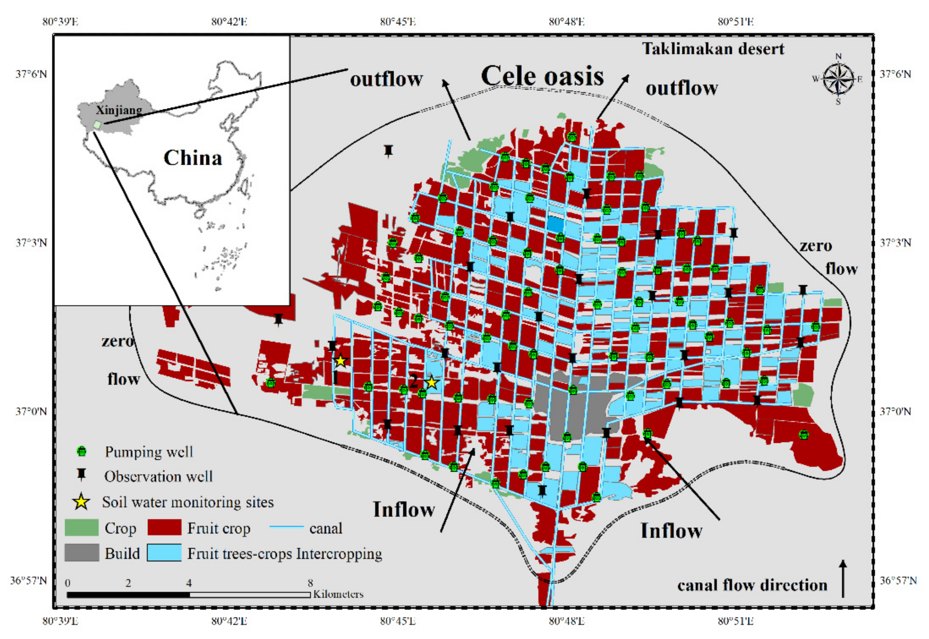
2.1. Study Area

The Cele Oasis lies at coordinates 36°54′–37°09′ N, 80°37′–80°59′ E: the total area between the main part of the oasis and the desert transition zone is 189.64 km2 [30], and the cultivated land area is 22,974.75 ha. The oasis is located on the southern edge of the Taklimakan Desert and the northern foot of the Kunlun Mountains, China; it has a typical continental arid desert climate and an average altitude of 3200 m in the mountains and 1500–1800 m in the plains.
The temperature here is largely different between day and night. The average annual precipitation is 35.5 mm, and the annual evaporation is 2751 mm. The annual average evaporation data come from the 20 cm evaporation pan data of the Cele Station from 1960 to 2010 [39]. The vegetation coverage is low and the ecological environment is very fragile. The Cele River provides a source of surface water for the evolution of the oasis, with an average annual runoff of 1.27 × 10⁸ m3, which flows into the extremely arid Taklimakan Desert.
The land use in the Cele Oasis is predominantly cropland, forest, and build. The cropland landscape covers about 9.6% of the total study area, forest covers 87.8%, and build land covers 13%. The main types of crops in Cele Oasis are red dates, walnuts, wheat, and corn. Crops typically are irrigated five or six times during the growth period, mostly from groundwater. (Figure 1).
The canal system inside the oasis is developed, forming a typical artificial farmland oasis landscape. The direction of flow of the groundwater aquifer in the oasis is the same as that of the surface flow. The buried depth of groundwater is less than 50 m, and the aquifer is a quaternary pore phreatic water system. The soil type in the study area is loamy sand, which has a high infiltration rate. In recent years, due to the impact of climate change and human activity, the agricultural cropping structure of the oasis has changed greatly, which has greatly affected the safety of the aquifer.

2.2. Data Sources

In this study, meteorological data from 2005–2017 were collected from the Cele National Station, taking into account the time-matching of groundwater data and meteorological data and using the FAO-56 Penman–Monteith method [40] to calculate the daily reference evapotranspiration. GF-1 remote sensing data (with a resolution of 2 m) were obtained from the China Resources Satellite Research Center (http://www.cresda.com/CN/ (accessed on 14 July 2016)). ENVI5.2 and ArcGIS software were used to preprocess the data. According to the land use/land cover classification system of the Chinese Academy of Sciences, a land use type map of the Cele Oasis was drawn using the supervised classification method. Fifty sample sites were randomly selected to test the accuracy of the classification results: the kappa coefficient was 0.92, which meets the standards of research accuracy. The Harmonized World Soil Datasets, version 1.2 (FAO/IIASA/ISRIC/ISS-CAS/JRC 2012) from the Food and Agriculture Organization (FAO) was used to obtain the bulk density and soil texture class for different profiles (https://eusoils.jrc.ec.europa.eu/ (accessed on 20 March 2009)). Groundwater level observation data from 25 wells in the area were obtained from Cele Hydrological Stations from 2005 to 2017. From 2012 to 2013, 4 independent hydrogeological surveys and borehole pumping tests were carried out in the 200-ha well-irrigation area in the region. After analyzing the pumping test data, the hydraulic conductivity and specific yield of the aquifer in the region were obtained. From 2015 to 2016, the soil moisture was monitored using soil temperature hygrometry at the field test site of the Cele National Station. The equipment provided automatic monitoring and the monitoring interval was set to 1 h. A hydrogeological map of the study area was obtained from the groundwater resource atlas of Xinjiang.

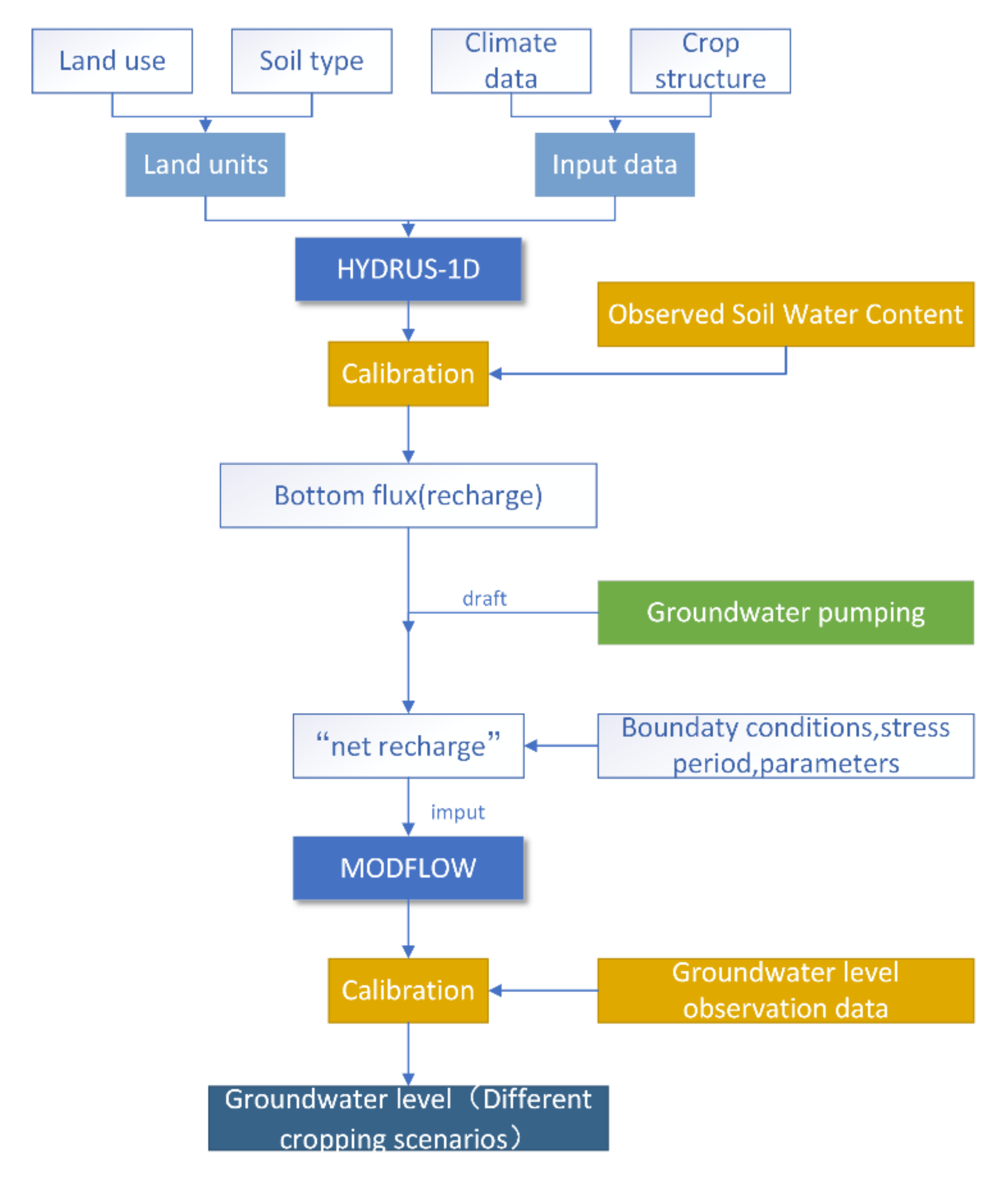
2.3. Modelling Description

HYDRUS-1D software [41] simulated the one-dimensional movement of water in variable-saturated porous media, soil moisture storage, and root water uptake. The model used a finite element numerical method to solve Richard’s equation of variable-saturated flow. In order to input the evapotranspiration (ET) and groundwater recharge calculated by HYDRUS-1D into the MODFLOW (cell) for data exchange, the study area was divided into different sites called “land units” according to the land use map and soil type map, and the recharge of different land type units was simulated. The main land use types in the oasis were cropland (9.6%), forest (87.7%), and build (2.7%). Loamy sand was the main soil type in the Cele Oasis. According to the land use type and soil type spatial distribution map, 3 simulations were constructed using HYDRUS-1D software for cropland loamy sand (CLS), forest loamy sand (FLS), and build loamy sand (BLS) (Table 1). Groundwater modeling system software (GMS), a type of modular three-dimensional steady-state finite difference software, was used to quantify the groundwater in the Cele Oasis.
The coupling modeling method of HYDRUS-1D and MODFLOW software used the drainage in the HYDRUS-1D model as the recharge in the MODFLOW model. The bottom flux calculated using the HYDRUS-1D model subtracted the pumping water from the well to obtain the “net recharge” of groundwater. The bottom boundary condition of the pressure head designated as HYDRUS-1D was used as the groundwater level in MODFLOW [42] to evaluate the influence of the vadose zone on groundwater fluctuation. Due to the deep groundwater in the arid area, the groundwater recharge of soil water in the unsaturated zone can be ignored for groundwater depths greater than 5 m. Therefore, we only considered the one-way process of groundwater recharge from the vadose zone in the Cele Oasis. The MODFLOW model divided the aquifer into blocks or grids and divided the soil or hydrogeological parameters into a region with similar parameters. Different regions corresponded to different HYDRUS-1D soil profiles. Figure 2 shows the coupling model of water flow through soil profile migration. Figure 3 shows a flow chart of the aquifer simulation using HYDRUS-1D and MODFLOW.

2.4. HYDRUS-1D Model

The HYDRUS-1D model is a one-dimensional vertical model, which simulates water, heat, solute transport, and root water uptake in vadose zones [43]. The model used Richard’s equation with added source-sink terms to solve for vertical soil moisture transport [44] (Equation (1)). The model assumed that air does not hinder the flow of water; in addition, the model used the van Genuchten equation [45] or the Brooks and Corey characteristic equation [46] to calculate the unsaturated soil hydraulic characteristics. Table 2 gives the soil hydraulic parameters of three land use types in the Cele Oasis. The one-dimensional Richard’s equation was given by:
θ t = z K h h z K h S
where θ is the volumetric water content (dimensionless), K is the hydraulic conductivity [L T−1], h is the soil water pressure head [L], t is time [T], z is the vertical coordinate [L], S is a sink term [T−1], and K(h) is the unsaturated hydraulic conductivity [L T−1]. The water content, θ (h), and the unsaturated hydraulic conductivity, K(h), made Richard’s equation a highly nonlinear equation that needed to be solved numerically.

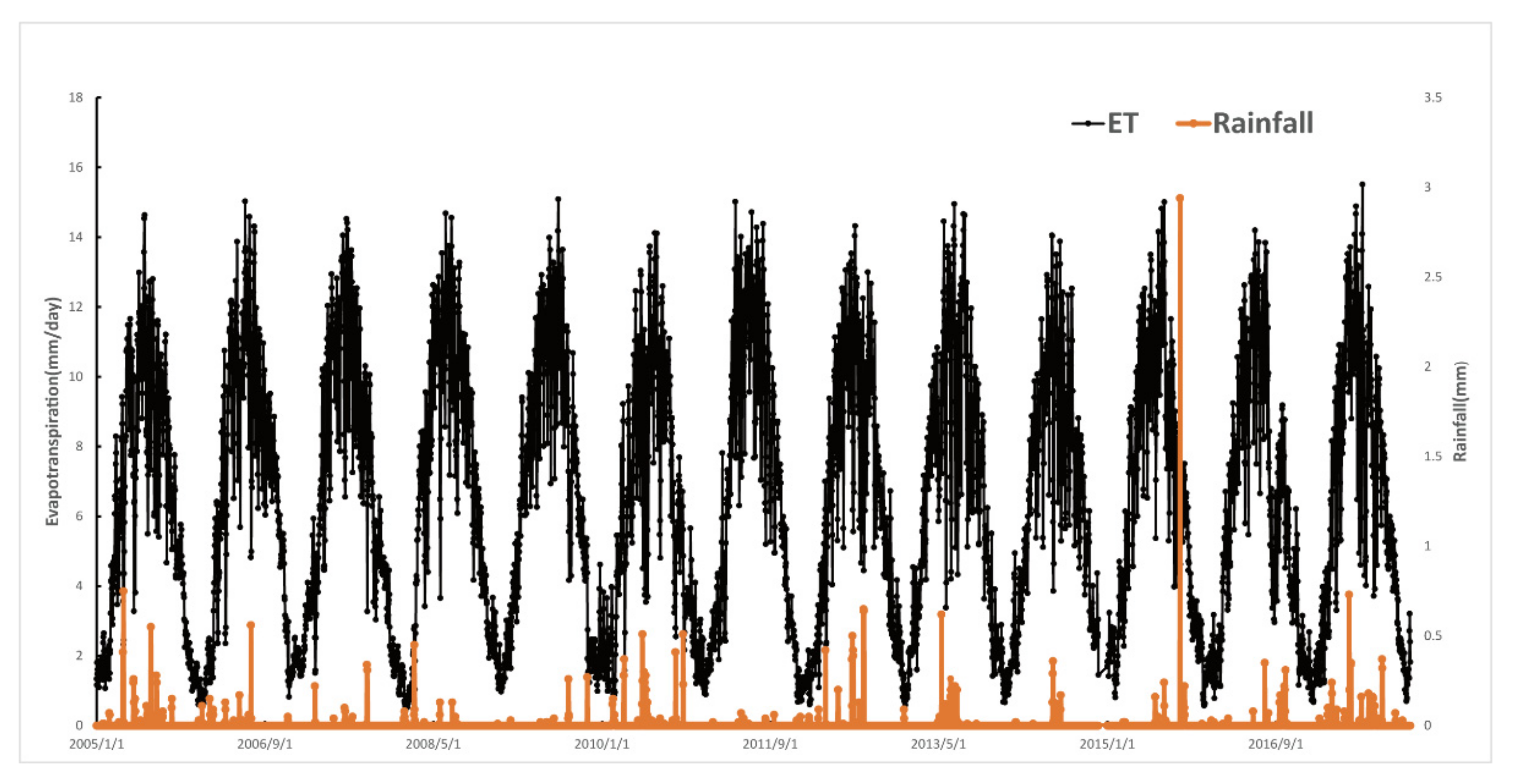
2.4.1. Evaporation and Transpiration

According to climate and soil parameters, ET0 was calculated using the Penman–Monteith model [47,48]. The potential evapotranspiration of crops was calculated using Equation (2):
E T P = K c × E T 0
where K c is the crop coefficient. According to FAO56, the values of K c in this paper were 0.4, 0.8, and 0.5, in the early stage (ground coverage is less than 10%), the middle stage (ground coverage is from 10% to maturity), and in the later stage (ground coverage is from maturity to harvest), respectively [40]. E T 0 was the reference evapotranspiration. E T 0 and precipitation from 2005 to 2017 are shown in Figure 4.
The HYDRUS-1D model calculated the soil evapotranspiration (Ep) and crop evapotranspiration (Tp) separately, given in Equations (3) and (4), respectively:
T p = E T P 1 e k × L A I
E P = E T P e k × L A I = E T P T P
where LAI is the leaf area index, and k is the canopy extinction coefficient.

2.4.2. Soil Hydraulic Parameters

From 2015 to 2016, a 2-m soil moisture monitoring experiment was carried out at the Cele National Station. Therefore, HYDRUS-1D used 2 m as the soil profile depth to simulate the bottom flux of each land unit and considered the soil texture in the Cele Oasis to be uniform; the hydraulic characteristics of the whole soil profile were also considered to be uniform. In the HYDRUS-1D model, the soil volume mass and soil particle size classification were the inputs, and parameters such as saturated water content θs, residual water content θr, and saturated hydraulic conductivity Ks were preliminarily determined using the Rosetta module of a neural network. Compared with the observed water data, the error between the simulated value and the measured value was reduced by adjusting the parameters. The results are shown in Table 2.

2.4.3. Root Water Uptake

HYDRUS-1D used a water stress response function to study root water uptake, and the Feddes model was used to calculate root water uptake [49]. The parameters in the root water uptake-water stress response function were taken from the HYDRUS-1D database [50].

2.4.4. Initial and Boundary Conditions

The initial condition of the HYDRUS-1D model was the initial measured value of soil moisture. The upper boundary used the atmospheric boundary of the surface integrated water, and meteorological data were used to specify the atmospheric boundary conditions. The lower boundary was located in the unsaturated zone because it did not reach the phreatic layer (the groundwater table depth is greater than 5 m), and it was set as the free drainage boundary.

2.5. MODFLOW Model

MODFLOW is one of the most widely used groundwater numerical simulation models and is a physical model. MODFLOW was combined with Darcy’s law and the groundwater flow equilibrium equation, using a finite difference method, to solve the groundwater motion equation. Using the MODFLOW module in GMS software, this paper constructed a MODFLOW model of the Cele Oasis [51] and solved the three-dimensional groundwater flow equation (Equation (5)) to obtain the head value.
x K x x h x + y K y y h y + z K z z h z w = S y h t
where K x x , K y y , and K z z are hydraulic conductivity coefficients (L/T) in the x-, y-, and z- directions, respectively; h is the hydraulic head (L); S y is the specific storage (1/L); and W is the recharge/discharge rate per unit volume (1/T).
In the MODFLOW finite difference method, continuous time and space were divided into a series of discrete blocks or grids, including horizontal and vertical subdivision grids. On the horizontal plane, the Cele Oasis was composed of 24,585 elements on a 200 m × 200 m grid, including 149 rows and 156 columns. The vertical profile of the aquifer was that of a single phreatic aquifer, and the simulation depth was (5–100 m), according to the groundwater level monitoring data and evaporation, and other related hydrological data. From 1 May 2005 to 30 April 2017, the time length was 4382 days, which was divided into 24 pressure periods. The pressure period was divided into a flood stress period (May–September) and a dry season stress period (October–April). The time step was one day. Therefore, the flood stress period was 153 days, and the dry season stress period was 212 days.

2.5.1. Model Parameters

According to the four pumping tests conducted from 2003–2004, Sy = 0.08, and the range of hydraulic conductivity of the aquifer in the Cele Oasis was 1.8–15 m/day. Both the annual total groundwater pumping amount and the monthly groundwater pumping amount in 2010 were obtained from the Cele County Water Resources Bureau and the China Statistical Yearbook of Water Resources (Xinjiang Volume 2005), combined with years of observation experience. Groundwater pumping accounted for 30% of the total amount of pumping water in the flood stress period, and 70% in the dry season stress period. The total amount of groundwater pumping in the flood stress period ranged from 0.00062 m/day in 2005 to 0.00065 m/day in 2017. The total amount of groundwater pumping during the dry season stress period ranged from 0.00104 m/day in 2005 to 0.00154 m/day in 2017. The source of groundwater recharge in the MODFLOW model was the HYDRUS-1D daily recharge flow (bottom flux) minus the pumping water to estimate the “net recharge”.

2.5.2. Initial and Boundary Conditions

According to the groundwater monitoring data of Cele Oasis in May 2005, the kriging interpolation method was used to interpolate 25 observations of well data in ArcGIS software to obtain the initial head. The upper boundary of the oasis is the phreatic surface, where the water exchange boundary with changing positions occurs, including irrigation infiltration and pumping wells. The lower boundary is bounded by a weak permeable layer, which is generalized as an impermeable boundary. The southern mountain outlet area is the flow boundary of lateral inflow. The eastern, northwestern, and northern areas are bound by underground watersheds, which are generalized as zero-flow boundaries. A small amount of lateral outflow is observed in some areas for lateral outflow boundary treatment.

2.5.3. Model Calibration

Observed data collected for 423 days, from 4 May 2016 to 30 April 2017, were selected to verify the HYDRUS-1D model. During this period, a total of 10 irrigation times were used. The observed values were compared with simulated values to verify the accuracy of the HYDRUS-1D model simulation. In the case of MODFLOW, the groundwater monitoring data of 25 observation wells, collected from 2005 to 2017, were used for model calibration, and the simulated and observed groundwater levels as functions of time were compared. The commonly used root mean square error (RMSE) [52] and the Nash–Sutcliffe model efficiency coefficient (NSE) [53] were used to evaluate the accuracy of the simulation results of the model. The RMSE and NSE are given by Equations (6) and (7), respectively.
R M S E = i = 1 n O i P i n 1
N S E = 1 i = 1 n P i O i 2 i = 1 n ( O i O ¯ ) 2
where O i and P i are the ith values of the observed and the simulated dataset, respectively, Ō is the average of the observed values, and n is the total number of observations.

2.6. Scenario Simulation

The industrial foundation of the Cele Oasis is weak, and the low-value-added crops grown there are mainly walnuts, red dates, and wheat. In order to promote the development of the Cele Oasis, the state implemented a policy of “targeted poverty alleviation”. Many institutions promote the improvement of cropping intensity, such as through “fruit trees-crops intercropping”, to drive agricultural production and improve residents’ income. However, this kind of “fruit trees-crops intercropping” increases the groundwater pumping capacity in the dry season (October–April). The long-term impact of this high-intensity groundwater extraction strategy during the drought period is still unclear. Therefore, this paper used 4 different cropping scenarios to evaluate the impact on groundwater. The first scenario was based on the current 100% cropping intensity. In the second, third, and fourth cropping scenarios, 105CI, 110CI, and 115CI were considered, respectively. The four different cropping scenarios assumed that the planting area of forest fruit crops remained unchanged: only the cropping area of wheat/maize changed. (Table 3).
The CropWat Model established by the Land and Water Development Division of FAO was used to calculate the increased irrigation water demand due to the expansion of planting areas. According to the irrigation water storage for different crops obtained from the experimental plot of the Cele Station, the monthly average irrigation water demand for forestry fruit crops was 1.5 × 10³ m3/hm2, and the monthly average irrigation water demand of wheat and maize was 1.05 × 10 m3/hm2. Equation (8) is used to calculate the water extraction of crops in the dry season for different cropping intensities:
D n m = C i A i × W R a u t u m n + w i n t e r 242
where C i is the planting area in scenario i, A t is the total area (ha), W R a u t u m n + w i n t e r is the sum of the crop irrigation water requirement in the dry season (mm), 242 is the number of drafting water days in the dry season, and D n m is the increased draft (mm/day) in scenario i.

3. Results

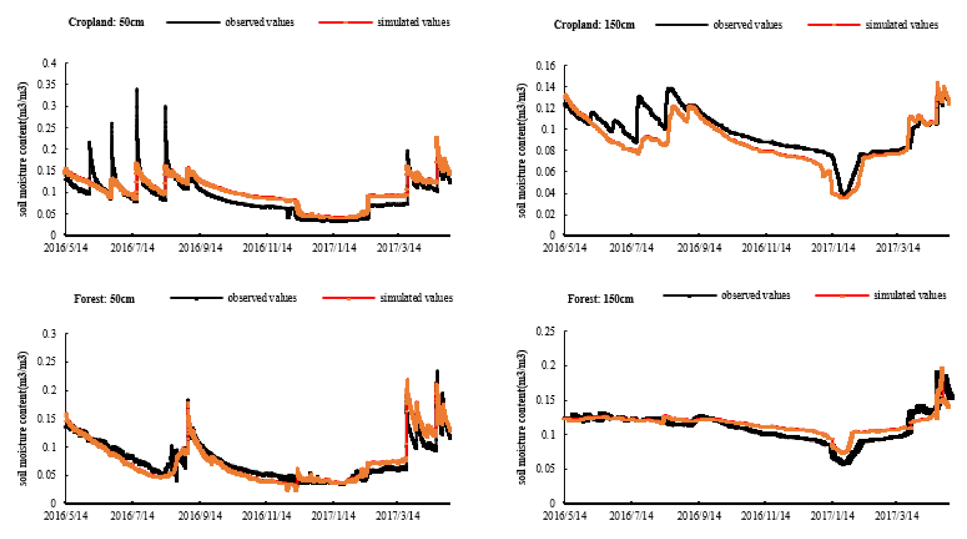
3.1. HYDRUS-1D Calibration Results and Recharge Flux

The HYDRUS-1D model was used to simulate the cropland and forest land units in the study area. The spatial location of soil water monitoring sites is shown in Figure 1. The HYDRUS-1D model was verified by selecting the observed data for 423 days, from 4 May 2016 to 30 April 2017. During this period, a total of 10 irrigations were conducted, in which the sudden increase in soil water content was expressed as irrigation. The soil water observations and simulation values of cropland and forest are shown in Figure 5. The models used 50 cm and 150 cm as examples.
Figure 5 shows that the observed water content and the model simulation results fit each other well. The soil water content increased rapidly after irrigation at 50 cm, whereas soil water content at 150 cm responded only two days after irrigation as the rate of change range was relatively small. Due to the complex soil environment, the NSE values between the simulated and observed values for soil water content in the shallow layers were 0.823 and 0.792, respectively, whereas the NSE values for the deep soil water content were 0.876 and 0.81. The fitting of the simulation values with the observed values was good. In terms of the RMSE, the simulation results for deep soil were better than those for shallow soil. In general, the HYDRUS-1D model had high simulation accuracy for soil moisture content. This model could, therefore, readily be used in the analysis of cropland and forest water migration and in the calculation of cropland and forest water supply to groundwater.
The simulation results showed that the largest cumulative recharge flux came from forest land (walnut, red date, pomegranate) (Table 4), mainly from irrigation infiltration recharge, as high evaporation loss in the Cele Oasis and field bunds prevented runoff from cropland and forest land. Compared to that of cropland and forest land units, the cumulative recharge flux from build land units was low. This is mainly due to hardened roads and a lack of precipitation recharge. Spatially, the bottom fluxes of different land units were fed into each model unit in MODFLOW.

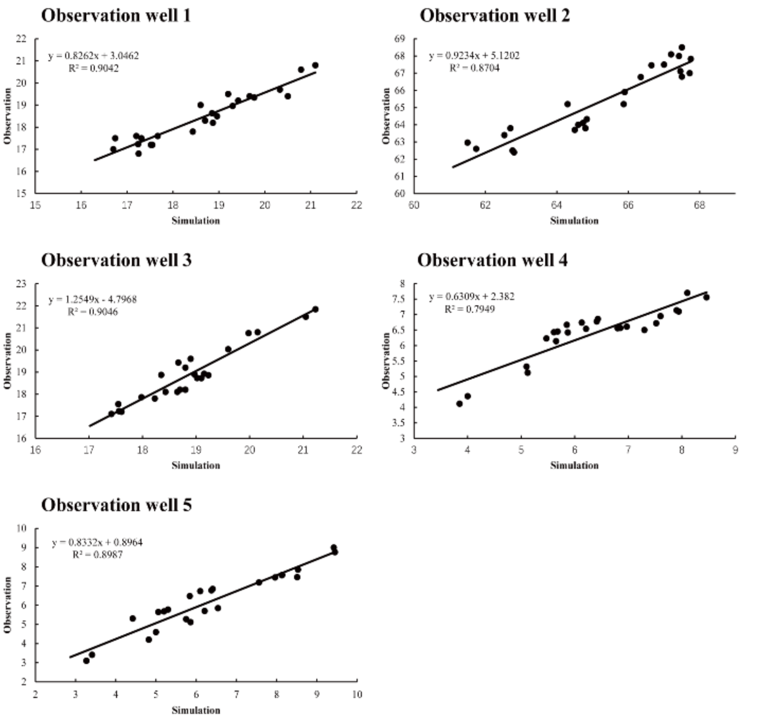
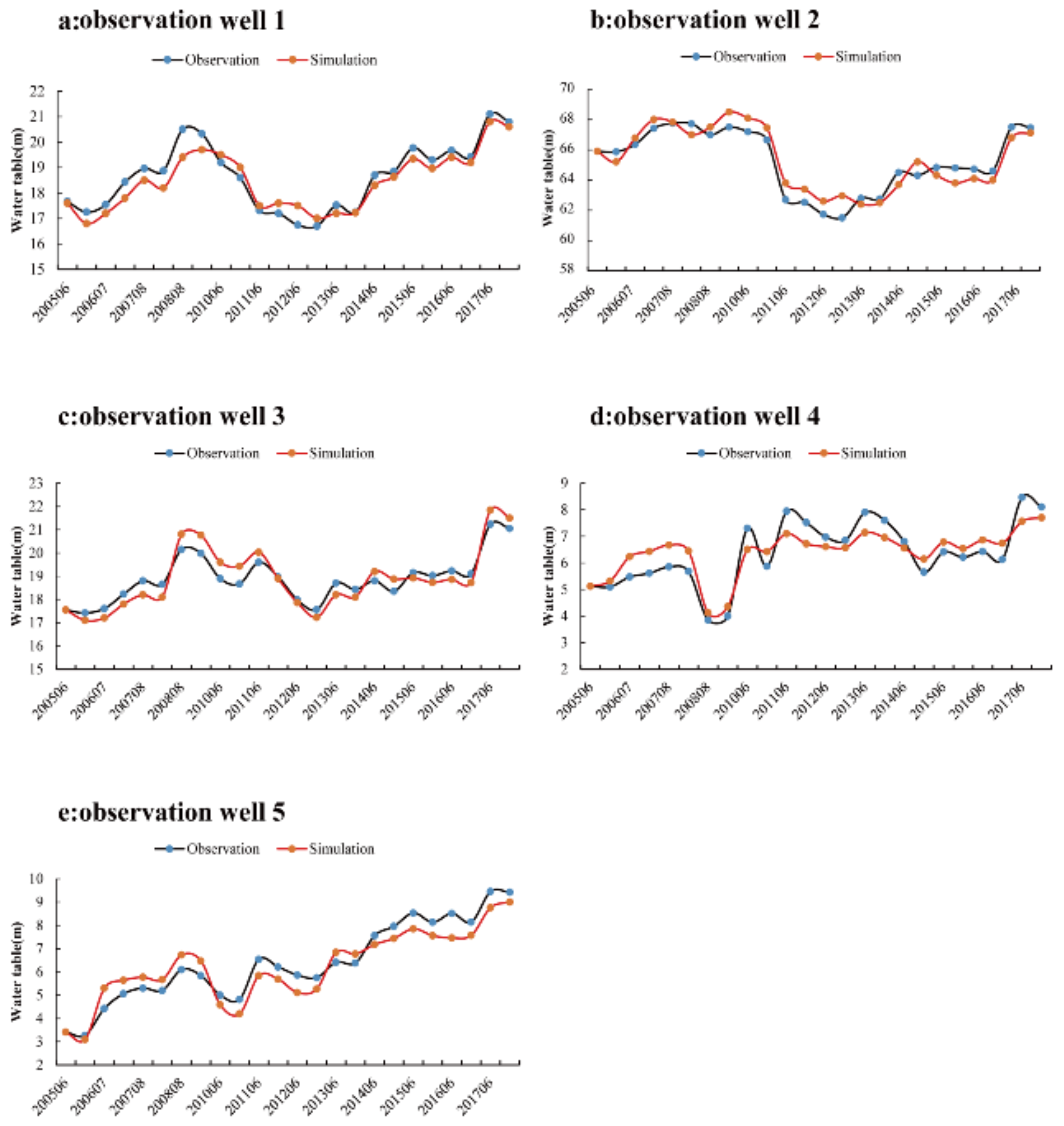
3.2. MODFLOW Calibration Results

The model correction needed to reflect the real groundwater level value. Therefore, the real groundwater level value of the observation well was input into the model, and the actual discharge of the pumping well was adjusted continuously; thus the simulated water level value was basically consistent with the water level value of 25 observation wells. The adjusted K value is shown in Figure 6a. The comparison between the calculated water level after model correction and the observed water level is shown in Figure 6b. Groundwater monitoring data from May 2005 to April 2017 were used to correct the simulated groundwater recharge in the cropping scenario (100CI). The observed data from 5 observation wells in the study area were compared with MODFLOW simulation data (Figure 6a). Figure 7 shows the observed and simulated head values of 5 representative observation wells at 1:1. Figure 8 shows the relationship between the simulated and observed average groundwater levels. As shown in Table 5, the ranges of R2 and RMSE, between the observed and simulated values, were 0.77–0.90 and 0.45–0.74 m, respectively. The lowest NSE value of well-3 and well-4 was 0.76, and the RMSE value of well-1 was highest at 0.74, indicating that the groundwater level simulated by the HYDRUS-1D and MODFLOW coupling models was consistent with the observed values. The simulation accuracy was high. Using GMS software to calculate the water budget of the Cele Oasis aquifer, the results showed that the recharge of the Cele Oasis water resources mainly consisted of melting water from alpine snow and ice, accounting for 96% of the total recharge. During the simulation period, the long-term average annual net inflow volume of the oasis was 1.3 × 10⁸ m3, whereas the long-term average annual net outflow volume was 1.33 × 10⁸ m3. This indicated that the Cele Oasis maintained a dynamic water balance under cropping intensity (100CI).

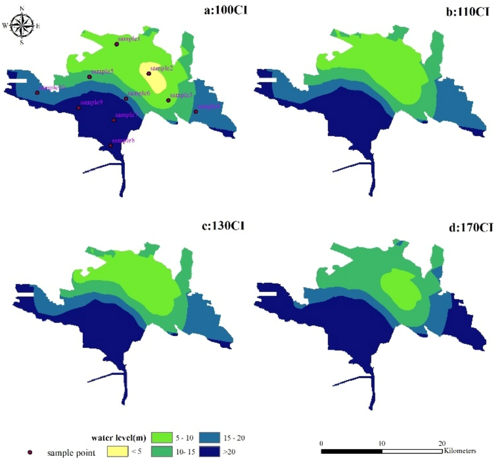
3.3. Effects of Different Cropping Scenarios on Groundwater Level

In order to examine the impacts of different cropping scenarios on the groundwater level, the average groundwater level of the flood period from May 2005 to April 2017 was used as the base year; under four different cropping scenarios, the groundwater level predicted by the flood period in April 2017 was compared with the base year to assess the impact of each cropping scenario on the groundwater level of the aquifer.
As compared to the base year, the spatial distribution of the groundwater level under different cropping scenarios is shown in Figure 9. Ten representative sites were selected (Figure 9a) to evaluate the fluctuation of groundwater level under different cropping scenarios (Table 6). Under the current cropping scenario, the groundwater level in 2017 was 0.23, 2.98 m lower than that in the base year. In the area where the water level was greater than 20 m, the surface water recharge was weak, which caused the water level fluctuation. In the area where the water level was less than 20 m, the surface water can effectively recharge the groundwater and make the groundwater level change only a little, which can be ignored. This indicates that there was considerable interaction between surface water and shallow groundwater. In general, the groundwater level in the Cele Oasis did not show a significant upward/downward trend from 2005 to 2017. This indicates that, under the current cropping intensity (100CI), the Cele Oasis maintains a dynamic water balance and that the sustainable development of the oasis remains stable. Figure 9a shows the spatial distribution of groundwater level in the oasis under the 100CI scenario.
The MODFLOW model was used to simulate groundwater level change for different cropping intensities in the Cele Oasis. The results are shown in Figure 9b–d and Table 6. With increasing cropping intensity (110CI, 130CI, and 170CI), the groundwater level in 2017 was significantly lower than that in the base year (2005). When the cropping intensity was 110%, 130%, and 170%, the groundwater level was 1.32–4.05 m, 2–4.54 m, and 3.09–7.07 m lower than that in the base year, respectively.
Figure 9 shows that when the cropping intensity was greater than 100%, the areas with a groundwater level less than 5 m disappeared. When the cropping intensity was 110% and 130%, the groundwater level does not have a significant decline. When the cropping intensity was 170%, the groundwater level of the oasis dropped rapidly and the area with a water level of 5–10 m was reduced by 208%, compared with the same water level in the 100CI scenario.

4. Discussion

4.1. Modeling Method

In this paper, HYDRUS-1D and MODFLOW models were used to evaluate the influence of long-term groundwater extraction from the Cele Oasis. The HYDRUS-1D model was used to simulate the soil water flow in cropland, forest land, and build land units. Due to the existence of the vadose zone, the exchange between the surface water and groundwater decreased [54]. The difficulties in numerical simulation of coupled flow systems in the vadose zone-saturated zone lie in the nonlinearity of the soil water model, the inhomogeneity of parameters, and the variability of hydrological stress [55,56,57]. These difficulties make the recharge of groundwater from soil water challenging to tackle in MODFLOW modeling [58], and sometimes time-consuming [59]. Mail [1] and Li et al. [59] demonstrated that HYDRUS-1D can accurately estimate groundwater recharge under different cropping conditions for different study areas. In this study, the recharge calculated by HYDRUS-1D for different land units was accurate and was close to the recharge calculated by Qian et al. [60]. HYDRUS-1D simulated soil water content at different depths and the NSE of the observed value was 0.82. This means that there was good agreement between the simulated value and the observed value.
The Cele Oasis is a typical piedmont alluvial plain. The influence of the deep groundwater level on the soil water in the vadose zone can be ignored, which makes the coupling of the vadose zone and the saturated zone become a single coupling. The bottom flux calculated from the HYDRUS-1D model subtracts the pumping water to obtain the “net recharge” of groundwater. The bottom boundary condition of the pressure head designated as HYDRUS-1D was used as the burial depth of the groundwater level in MODFLOW [42] to evaluate the influence of the vadose zone on groundwater fluctuation. The MODFLOW model simulation results were consistent with those of Liu et al. [61], who used an optimization algorithm to calculate groundwater level in the Cele Oasis.

4.2. Increased Cropping Intensity: Enlightenment and Strategies

In arid and semi-arid regions, oases play a vital role in human survival and development. The main industry in oases, agriculture, places a very high demand on groundwater compared with agriculture in other regions [62]. Due to the implementation of the “targeted poverty alleviation” policy, how to increase the cropping intensity and economic development in oases with minimal damage to their sustainable development has become paramount. The results also show that the Cele Oasis needs to maintain a long-term balance between water consumption and water availability, while addressing the shortage of water resources caused by increased cropping intensity.
With improvements in drilling technology and the popularization of high-power pumping pumps, unplanned groundwater extraction causes serious waste of groundwater resources. It leads to an unsustainable groundwater system in the short term [63]. Groundwater management, especially groundwater management in oases, is an increasingly important issue. In this context, the results of this study could be used to optimize the layout of pumping wells in oases, so as to realize the sustainable utilization of groundwater in irrigation areas [64,65].
The Cele River is the main source of surface water in the Cele Oasis, with an annual average net inflow volume of 1.2 × 10⁸ m3. However, more than 59.5% of the irrigation water in the region is from groundwater [60]. The results of this study show that increasing cropping intensity will lead to the unsustainable development of groundwater in the oasis, and that the combined use of surface water and groundwater will help to alleviate shortages of groundwater in the oasis. Liu [61] and Ma et al. [66] improved the layout of pumping wells using optimization algorithms, but there are still pumping wells being overused, leading to serious groundwater extraction. This result predicts that increases in cropping intensity in the future will lead to a significant decline in groundwater levels. Therefore, it is necessary to allocate surface water, improve water conveyance networks, and boost irrigation efficiency so as to ensure the sustainable development of groundwater resources. The average annual runoff of the Cele River is 1.2 × 10⁸ m3, but a large amount of the surface water flows out of the Cele Oasis each year during the flood period which could be used as a potential source of groundwater recharge. Therefore, it is necessary to construct water conservancy projects in the Cele Oasis for groundwater recharge and agricultural irrigation.

5. Conclusions

HYDRUS-1D and MODFLOW models were used to evaluate the effects of different cropping intensities on groundwater in the Cele Oasis. HYDRUS-1D was used to simulate soil moisture migration in the vadose zone, and the cumulative bottom fluxes of different land use units (cropland, forest, build) from 2005 to 2017 were estimated. The results showed that the bottom fluxes of forest land were higher than those of cropland, and the bottom fluxes of build land were the lowest. The bottom fluxes of the three types of units were 43.2 mm, 159.6 mm, and 4.8 mm, respectively. The bottom fluxes of the three types of units were used as a recharge source for MODFLOW. By comparing the observed groundwater level data with the simulated data, it was found that MODFLOW accurately simulated groundwater level change. This indicates that the HYDRUS-1D and MODFLOW models successfully simulated the interaction between soil water and groundwater in the Cele Oasis. By comparing the effects of different cropping intensities on groundwater, the results showed that there was no significant change in the groundwater level under the current cropping intensity (100CI) scenario. When the cropping intensity increased to 110% and 130%, the groundwater level decreased slightly, and the maximum drawdown depth was 1.56 m. When the cropping intensity reached 170%, the groundwater level decreased significantly. The results indicated that the maximum degree of agricultural intensification in the Cele Oasis was 130% of the current cropping intensity. When it was greater than 130%, the groundwater in the Cele Oasis was not compensated by irrigation water, resulting in a sharp drop in the water level and leading to concerns about the groundwater safety and stability of the oasis. The spatial distribution of the groundwater level in the oasis shows that the northwest region is more vulnerable to increases in groundwater exploitation. Therefore, in the process of agricultural intensification, attention should be paid to ecological security, especially in an oasis area with a fragile ecological environment in an arid region.

Author Contributions

Conceptualization, D.X. and H.D.; methodology, D.X. and Y.L. (Yunfei Liu); data curation, Y.L. (Yi Liu), L.Z. and W.L.; writing—original draft preparation, D.X.; writing—review and editing, H.D.; project administration, H.D. and Y.L. (Yi Liu); funding acquisition, H.D. All authors have read and agreed to the published version of the manuscript.

Funding

This research was funded by the National Natural Science Foundation of China, grant number 42171042, and Western Light—western region leading scientists supporting project, Chinese Academy of Sciences, grant number 2018-XBYJRC-002.

Institutional Review Board Statement

Not applicable.

Informed Consent Statement

Not applicable.

Data Availability Statement

The data presented in this study are available upon reasonable request from the corresponding author.

Conflicts of Interest

The authors declare no conflict of interest.

References

  1. Mali, S.S.; Scobie, M.; Schmidt, E.; Okwany, R.O.; Kumar, A.; Islam, A.; Bhatt, B.P. Modelling vadose zone flows and groundwater dynamics of alluvial aquifers in Eastern Gangetic Plains of India: Evaluating the effects of agricultural intensification. Environ. Earth Sci. 2021, 80, 19. [Google Scholar] [CrossRef]
  2. Fienen, M.N.; Arshad, M. The International Scale of the Groundwater Issue. In Integrated Groundwater Management: Concepts, Approaches and Challenges; Jakeman, A.J., Hunt, R.J., Rinaudo, J.D., Eds.; Springer International Publishing: Cham, Switzerland, 2016; pp. 21–48. [Google Scholar]
  3. Siebert, S.; Burke, J.; Faures, J.M.; Frenken, K.; Hoogeveen, J.; Döll, P.; Portmann, F.T. Groundwater use for irrigation—A global inventory. Hydrol. Earth Syst. Sci. 2010, 14, 1863–1880. [Google Scholar] [CrossRef] [Green Version]
  4. Casanova, J.; Devau, N.; Pettenati, M. Managed Aquifer Recharge: An Overview of Issues and Options. In Integrated Groundwater Management: Concepts, Approaches and Challenges; Jakeman, A.J., Hunt, R.J., Rinaudo, J.D., Eds.; Springer International Publishing: Cham, Switzerland, 2016; pp. 413–434. [Google Scholar]
  5. Foster, S.; Chilton, J.; Nijsten, G.J.; Richts, A. Groundwater—A global focus on the ‘local resource’. Curr. Opin. Environ. Sustain. 2013, 5, 685–695. [Google Scholar] [CrossRef]
  6. Brown, T.C.; Foti, R.; Ramirez, J.A. Projected freshwater withdrawals in the United States under a changing climate. Water Resour. Res. 2013, 49, 1259–1276. [Google Scholar] [CrossRef]
  7. Sauer, T.; Havlik, P.; Schneider, U.; Schmid, E.; Kindermann, G.E.; Obersteiner, M. Agriculture and resource availability in a changing world: The role of irrigation. Water Resour. Res. 2010, 46, 12. [Google Scholar] [CrossRef] [Green Version]
  8. Vélez-Nicolás, M.; García-López, S.; Ruiz-Ortiz, V.; Sánchez-Bellón, Á. Towards a Sustainable and Adaptive Groundwater Management: Lessons from the Benalup Aquifer (Southern Spain). Sustainability 2020, 12, 5215. [Google Scholar] [CrossRef]
  9. Arora, B.; Dwivedi, D.; Faybishenko, B.; Jana, R.B.; Wainwright, H.M. Understanding and Predicting Vadose Zone Processes. In Reactive Transport in Natural and Engineered Systems; Druhan, J.L., Tournassat, C., Eds.; Mineralogical Society of America and The Geochemical Society: Chantilly, VA, USA, 2019; pp. 303–328. [Google Scholar]
  10. Zeng, J.; Guo, B. Multidimensional simulation of PFAS transport and leaching in the vadose zone: Impact of surfactant-induced flow and subsurface heterogeneities. Adv. Water Resour. 2021, 155, 18. [Google Scholar] [CrossRef]
  11. Ng, G.-H.; McLaughlin, D.; Entekhabi, D.; Scanlon, B. Using data assimilation to identify diffuse recharge mechanisms from chemical and physical data in the unsaturated zone. Water Resour. Res. 2009, 45, 18. [Google Scholar] [CrossRef] [Green Version]
  12. Smerdon, B.D.; Allen, D.; Neilsen, D. Evaluating the use of a gridded climate surface for modelling groundwater recharge in a semi-arid region (Okanagan Basin, Canada). Hydrol. Process. 2010, 24, 3087–3100. [Google Scholar] [CrossRef]
  13. Kim, J.H.; Jackson, R.B. A Global Analysis of Groundwater Recharge for Vegetation, Climate, and Soils. Vadose Zone J. 2012, 11. [Google Scholar] [CrossRef] [Green Version]
  14. Lyu, S.; Chen, W.; Wen, X.; Chang, A.C. Integration of HYDRUS-1D and MODFLOW for evaluating the dynamics of salts and nitrogen in groundwater under long-term reclaimed water irrigation. Irrig. Sci. 2019, 37, 35–47. [Google Scholar] [CrossRef]
  15. Scanlon, B.R.; Healy, R.W.; Cook, P.G. Choosing appropriate techniques for quantifying groundwater recharge. Hydrogeol. J. 2002, 10, 18–39. [Google Scholar] [CrossRef]
  16. Kassaye, K.T.; Boulange, J.; Tu, L.H.; Saito, H.; Watanabe, H. Soil water content and soil temperature modeling in a vadose zone of Andosol under temperate monsoon climate. Geoderma 2021, 384, 14. [Google Scholar] [CrossRef]
  17. Gurwin, J. Ocena Odnawialności Struktur Wodonośnych Bloku Przedsudeckiego. Integracja Danych Monitoringowych i GIS/RS z Numerycznymi Modelami Filtracji [Renewal Assessment of Water-Bearing Structures within the Fore-Sudetic Block. Integration of Monitoring and GIS/RS Data with Numerical Flow Models]; Wydawnictwo Uniwersytetu Wrocławskiego: Wroclaw, Poland, 2010; p. 218. [Google Scholar]
  18. Dabach, S.; Lazarovitch, N.; Šimůnek, J.; Shani, U. Numerical Investigation of Irrigation Scheduling Based on Soil Water Status. Irrig. Sci. 2013, 31, 27–36. [Google Scholar] [CrossRef]
  19. Szymkiewicz, A.; Savard, J.; Jaworska-Szulc, B. Numerical Analysis of Recharge Rates and Contaminant Travel Time in Layered Unsaturated Soils. Water 2019, 11, 545. [Google Scholar] [CrossRef] [Green Version]
  20. Tonkul, S.; Baba, A.; Şimşek, C.; Durukan, S.; Demirkesen, A.C.; Tayfur, G. Groundwater Recharge Estimation Using HYDRUS 1D Model in Alaşehir Sub-Basin of Gediz Basin in Turkey. Environ. Monit. Assess. 2019, 191, 610. [Google Scholar] [CrossRef]
  21. Neto, D.C.; Chang, H.K.; van Genuchten, M.T. A Mathematical View of Water Table Fluctuations in a Shallow Aquifer in Brazil. Groundwater 2016, 54, 82–91. [Google Scholar] [CrossRef]
  22. Dafny, E.; Šimůnek, J. Infiltration in layered loessial deposits: Revised numerical simulations and recharge assessment. J. Hydrol. 2016, 538, 339–354. [Google Scholar] [CrossRef] [Green Version]
  23. Kendy, E.; Bredehoeft, J.D. Transient effects of groundwater pumping and surface-water-irrigation returns on streamflow. Water Resour. Res. 2006, 42. [Google Scholar] [CrossRef]
  24. Currie, D.; Laattoe, T.; Walker, G.; Woods, J.; Smith, T.; Bushaway, K. Modelling Groundwater Returns to Streams From Irrigation Areas with Perched Water Tables. Water 2020, 12, 956. [Google Scholar] [CrossRef] [Green Version]
  25. Boyce, S.E.; Nishikawa, T.; Yeh, W.W.-G. Reduced order modeling of the Newton formulation of MODFLOW to solve unconfined groundwater flow. Adv. Water Resour. 2015, 83, 250–262. [Google Scholar] [CrossRef] [Green Version]
  26. Havard, P.L.; Prasher, S.O.; Bonnell, R.; Madani, A. Linkflow, a Water Flow Computer Model for Water Table Management: Part I. Model Development. Trans. ASAE 1995, 38, 481–488. [Google Scholar] [CrossRef]
  27. Facchi, A.; Ortuani, B.; Maggi, D.; Gandolfi, C. Coupled SVAT–groundwater model for water resources simulation in irrigated alluvial plains. Environ. Model. Softw. 2004, 19, 1053–1063. [Google Scholar] [CrossRef]
  28. Xu, X.; Huang, G.; Zhan, H.; Qu, Z.; Huang, Q. Integration of SWAP and MODFLOW-2000 for modeling groundwater dynamics in shallow water table areas. J. Hydrol. 2012, 412, 170–181. [Google Scholar] [CrossRef]
  29. Hao, X.M.; Li, W.H. Oasis cold island effect and its influence on air temperature: A case study of Tarim Basin, Northwest China. J. Arid Land 2016, 8, 172–183. [Google Scholar] [CrossRef] [Green Version]
  30. Xue, J.; Gui, D.; Zhao, Y.; Lei, J.; Zeng, F.; Feng, X.; Mao, D.; Shareef, M. A decision-making framework to model environmental flow requirements in oasis areas using Bayesian networks. J. Hydrol. 2016, 540, 1209–1222. [Google Scholar] [CrossRef]
  31. Chen, Y.; Yang, G.; Zhou, L.; Liao, J.; Wei, X. Quantitative Analysis of Natural and Human Factors of Oasis Change in the Tail of Shiyang River over the Past 60 Years. Acta Geol. Sin.-Engl. Ed. 2020, 94, 637–645. [Google Scholar] [CrossRef]
  32. Dassi, L.; Tarki, M.; El Mejri, H.; Ben Hammadi, M. Effect of overpumping and irrigation stress on hydrochemistry and hydrodynamics of a Saharan oasis groundwater system. Hydrol. Sci. J.-J. Sci. Hydrol. 2018, 63, 227–250. [Google Scholar] [CrossRef]
  33. Xue, J.; Huang, C.; Chang, J.; Sun, H.; Zeng, F.; Lei, J.; Liu, G. Water use efficiencies, economic tradeoffs, and portfolio optimizations of diversification farm systems in a desert oasis of Northwest China. Agrofor. Syst. 2021, 95, 1703–1718. [Google Scholar] [CrossRef]
  34. Colaizzi, P.D.; Gowda, P.H.; Marek, T.H.; Porter, D.O. Irrigation in the texas high plains: A brief history and potential reductions in demand. Irrig. Drain. 2009, 58, 257–274. [Google Scholar] [CrossRef]
  35. Chen, S.; Yang, W.; Huo, Z.; Huang, G. Groundwater simulation for efficient water resources management in Zhangye Oasis, Northwest China. Environ. Earth Sci. 2016, 75, 13. [Google Scholar] [CrossRef]
  36. Zhu, X.; Wu, J.; Nie, H.; Guo, F.; Wu, J.; Chen, K.; Liao, P.; Xu, H.; Zeng, X. Quantitative assessment of the impact of an inter-basin surface-water transfer project on the groundwater flow and groundwater-dependent eco-environment in an oasis in arid northwestern China. Hydrogeol. J. 2018, 26, 1475–1485. [Google Scholar] [CrossRef]
  37. Yao, Y.; Zheng, C.; Liu, J.; Cao, G.; Xiao, H.; Li, H.; Li, W. Conceptual and numerical models for groundwater flow in an arid inland river basin. Hydrol. Process. 2015, 29, 1480–1492. [Google Scholar] [CrossRef]
  38. Yang, G.; Tian, L.; Li, X.; He, X.; Gao, Y.; Li, F.; Xue, L.; Li, P. Numerical assessment of the effect of water-saving irrigation on the water cycle at the Manas River Basin oasis, China. Sci. Total Environ. 2020, 707, 8. [Google Scholar] [CrossRef]
  39. Rumbaur, C.; Thevs, N.; Disse, M.; Ahlheim, M.; Brieden, A.; Cyffka, B.; Duethmann, D.; Feike, T.; Frör, O.; Gärtner, P.; et al. Sustainable management of river oases along the Tarim River (SuMaRiO) in Northwest China under conditions of climate change. Earth Syst. Dyn. 2015, 6, 83–107. [Google Scholar] [CrossRef] [Green Version]
  40. Allen, R.G.; Pereira, L.S.; Raes, D.; Smith, M. Crop Evapotranspiration-Guidelines for Computing Crop Water Requirements-FAO Irrigation and Drainage Paper 56; FAO: Rome, Italy, 1998; Volume 300, p. D05109. [Google Scholar]
  41. Rassam, D.; Šimůnek, J.; Mallants, D.; van Genuchten, M.T. The HYDRUS-1D Software Package for Simulating the Movement of Water, Heat, and Multiple Solutes in Variably Saturated Media: Tutorial; CSIRO Land and Water: Canberra, Australia, 2018; p. 183. [Google Scholar]
  42. Twarakavi, N.K.C.; Šimůnek, J.; Seo, S. Evaluating interactions between groundwater and vadose zone using the HYDRUS-based flow package for MODFLOW. Vadose Zone J. 2008, 7, 757–768. [Google Scholar] [CrossRef] [Green Version]
  43. Šimůnek, J.; van Genuchten, M.T.; Šejna, M. Recent Developments and Applications of the HYDRUS Computer Software Packages. Vadose Zone J. 2016, 15, 25. [Google Scholar] [CrossRef] [Green Version]
  44. Ren, D.; Xu, X.; Hao, Y.; Huang, G. Modeling and assessing field irrigation water use in a canal system of Hetao, upper Yellow River basin: Application to maize, sunflower and watermelon. J. Hydrol. 2016, 532, 122–139. [Google Scholar] [CrossRef]
  45. Vangenuchten, M.T. A closed-form equation for predicting the hydraulic conductivity of unsaturated soils. Soil Sci. Soc. Am. J. 1980, 44, 892–898. [Google Scholar] [CrossRef] [Green Version]
  46. Mualem, Y. New model for predicting hydraulic conductivity of unsaturated porous-media. Water Resour. Res. 1976, 12, 513–522. [Google Scholar] [CrossRef] [Green Version]
  47. Wang, K.C.; Dickinson, R.E. A review of global terrestrial evapotranspiration: Observation, modeling, climatology, and climatic variability. Rev. Geophys. 2012, 50. [Google Scholar] [CrossRef]
  48. Ahmadi, S.H.; Javanbakht, Z. Assessing the physical and empirical reference evapotranspiration (ETo) models and time series analyses of the influencing weather variables on ETo in a semi-arid area. J. Environ. Manag. 2020, 276, 111278. [Google Scholar] [CrossRef]
  49. Ritchie, J.T. Model for predicting evaporation from a row crop with incomplete cover. Water Resour. Res. 1972, 8, 1204–1213. [Google Scholar] [CrossRef] [Green Version]
  50. Van den Broek, B.J.; van Dam, J.C.; Elbers, J.A.; Feddes, R.A.; Huygen, J.; Kabat, P.; Wesseling, J.G. SWATRE: Instructions for input; Internal Note; Winand Staring Centre: Wageningen, The Netherlands, 1991. [Google Scholar]
  51. McDonald, M.G.; Harbaugh, A.W. A modular three-dimensional finite difference ground-water flow model. In Techniques of Water-Resources Investigations; U.S. Geological Survey: Washington, DC, USA, 1988; p. 588. [Google Scholar]
  52. Chai, T.; Draxler, R.R. Root mean square error (RMSE) or mean absolute error (MAE)?—Arguments against avoiding RMSE in the literature. Geosci. Model Dev. 2014, 7, 1247–1250. [Google Scholar] [CrossRef] [Green Version]
  53. Woertgen, C.; Rothoerl, R.D.; Holzschuh, M.; Metz, C.; Brawanski, A. Comparison of serial S-100 and NSE serum measurements after severe head injury. Acta Neurochir. 1997, 139, 1161–1164. [Google Scholar] [CrossRef] [PubMed]
  54. Kong, J.; Xin, P.; Hua, G.-F.; Luo, Z.-Y.; Shen, C.-J.; Chen, D.; Li, L. Effects of vadose zone on groundwater table fluctuations in unconfined aquifers. J. Hydrol. 2015, 528, 397–407. [Google Scholar] [CrossRef]
  55. Zha, Y.; Yang, J.; Yin, L.; Zhang, Y.; Zeng, W.; Shi, L. A modified Picard iteration scheme for overcoming numerical difficulties of simulating infiltration into dry soil. J. Hydrol. 2017, 551, 56–69. [Google Scholar] [CrossRef]
  56. Krabbenhøft, K. An alternative to primary variable switching in saturated–unsaturated flow computations. Adv. Water Resour. 2007, 30, 483–492. [Google Scholar] [CrossRef]
  57. Zeng, J.; Yang, J.; Zha, Y.; Shi, L. Capturing soil-water and groundwater interactions with an iterative feedback coupling scheme: New HYDRUS package for MODFLOW. Hydrol. Earth Syst. Sci. 2019, 23, 637–655. [Google Scholar] [CrossRef] [Green Version]
  58. Ali, R.; McFarlane, D.; Varma, S.; Dawes, W.; Emelyanova, I.; Hodgson, G.; Charles, S. Potential climate change impacts on groundwater resources of south-western Australia. J. Hydrol. 2012, 475, 456–472. [Google Scholar] [CrossRef]
  59. Li, Y.; Šimůnek, J.; Jing, L.; Zhang, Z.; Ni, L. Evaluation of water movement and water losses in a direct-seeded-rice field experiment using Hydrus-1D. Agric. Water Manag. 2014, 142, 38–46. [Google Scholar] [CrossRef] [Green Version]
  60. Qian, J.P.; Zhao, J.P.; Gui, D.W.; Feng, X. Effects of Ecological Water Use and Irrigation on Groundwater Depth in Cele Oasis. Bull. Soil Water Conserv. 2018, 38, 96–102. [Google Scholar]
  61. Liu, Y.; Shen, M.; Zhao, J.; Dai, H.; Gui, D.; Feng, X.; Ju, J.; Sang, S.; Zhang, X.; Hu, B. A New Optimization Method for the Layout of Pumping Wells in Oases: Application in the Qira Oasis, Northwest China. Water 2019, 11, 970. [Google Scholar] [CrossRef] [Green Version]
  62. Ling, H.; Xu, H.; Shi, W.; Zhang, Q. Regional climate change and its effects on the runoff of Manas River, Xinjiang, China. Environ. Earth Sci. 2011, 64, 2203–2213. [Google Scholar] [CrossRef]
  63. Bekri, E.; Disse, M.; Yannopoulos, P. Optimizing water allocation under uncertain system conditions for water and agriculture future scenarios in Alfeios River Basin (Greece)—Part B: Fuzzy-boundary intervals combined with multi-stage stochastic programming model. Water 2015, 7, 6427–6466. [Google Scholar] [CrossRef] [Green Version]
  64. Campana, P.E.; Olsson, A.; Li, H.; Yan, J. An economic analysis of photovoltaic water pumping irrigation systems. Int. J. Green Energy 2016, 13, 831–839. [Google Scholar] [CrossRef]
  65. Ketabchi, H.; Ataie-Ashtiani, B. Ataie-Ashtiani, Coastal groundwater optimization—advances, challenges, and practical solutions. Hydrogeol. J. 2015, 23, 1129–1154. [Google Scholar] [CrossRef]
  66. Ma, T.; Wang, J.; Liu, Y.; Sun, H.; Gui, D.; Xue, J. A Mixed Integer Linear Programming Method for Optimizing Layout of Irrigated Pumping Well in Oasis. Water 2019, 11, 1185. [Google Scholar] [CrossRef] [Green Version]
Figure 1. Location of the study area (Cele Oasis) and division areas of cropping structure.
Agriculture 12 00641 g001
Figure 2. Conceptual framework for simulating water transport in vadose zones and aquifers using HYDRUS-1D and MODFLOW models.
Agriculture 12 00641 g002
Figure 3. Flow chart of the aquifer simulation using HYDRUS-1D and MODFLOW.
Agriculture 12 00641 g003
Figure 4. Rainfall and daily reference evapotranspiration from the simulation period (2005–2017).
Agriculture 12 00641 g004
Figure 5. Comparison of simulated and observed soil water content (cropland, forest).
Agriculture 12 00641 g005
Figure 6. Comparison of the observation well and the water level in the model under steady-state conditions. (a): Spatial distribution of hydraulic conductivity in shallow aquifers. (b): Water level comparison between observation well and model under steady state condition.
Agriculture 12 00641 g006
Figure 7. Observation wells 1–5, scatter plots of groundwater level of observed and simulated values in the study area.
Agriculture 12 00641 g007
Figure 8. (ae) Time comparison of groundwater level elevation observed and simulated by 5 observation wells during calibration period.
Agriculture 12 00641 g008
Figure 9. (ad) Spatial distribution maps of groundwater level in 2017 under different cropping intensity scenarios, (a) Current cropping intensity (100%), (b) 110% cropping intensity, (c) 130% cropping intensity, (d) 170% cropping intensity.
Agriculture 12 00641 g009
Table 1. Area of different land units.
Soil TypeLand UseLand UnitArea (km2)
Loamy sandCroplandCLS10.28
ForestFLS93.99
BuildBLS2.87
total 107.14
Table 2. The van Genuchten (1980) soil hydraulic parameters for the loamy sand in the Cele Oasis.
Land UseSoil Typeθr
(cm3cm−3)
θs
(cm3cm−3)
α
(cm−3)
nKs
(cm day−1)
l
CroplandLoamy sand0.060.5240.0311.57102.30.5
ForestLoamy sand0.0610.4320.0261.647.50.5
BuildLoamy sand0.0730.4260.0281.561.30.5
Note: θr is the soil residual water content, θs is the soil saturated water content, α and n are curve fitting parameters, Ks is the saturated hydraulic conductivity, and l is the molecular diffusion coefficient.
Table 3. Crop area under different model scenarios.
Model
Scenarios
Crop
Intensity
SummerAutumnWinter
Forestry
Fruit
Wheat *Maize *Forestry
Fruit
WheatMaizeForestry
Fruit
WheatMaize
100CI10090 km210 km2090 km2010 km290 km210 km20
110CI11090 km220 km2090 km2020 km290 km220 km20
130CI13090 km240 km2090 km2040 km290 km240 km20
170CI17090 km280 km2090 km2080 km290 km280 km20
* Wheat and maize are successional crops: wheat (November–June), maize (July–October).
Table 4. Cumulative recharge fluxes of different simulation units from May 2005 to April 2017.
Soil TypeLand UseRunoff (mm)Root-Water Uptake (mm)Bottom Flux (mm)
Loam sandCropland057.643.2
Forest0312159.6
Build19.76-4.8
Table 5. Error indicators between observed groundwater level and simulated value in different distribution areas.
Observation WellR2RMSENSE
Well-10.900.450.87
Well-20.870.740.86
Well-30.870.470.76
Well-40.770.590.76
Well-50.890.580.85
Table 6. Fluctuations of groundwater levels compared with base year.
Random
Sample
Base Year100CI110CI130CI170CI
Sample 17.020.251.411.654.21
Sample 24.370.231.791.574.33
Sample 37.960.341.911.734.07
Sample 414.51.292.872.775.55
Sample 512.40.651.322.004.16
Sample 617.520.811.612.154.43
Sample 742.32.984.054.547.07
Sample 855.312.543.433.895.41
Sample 923.12.843.694.153.09
Sample 1015.821.442.152.835.06
Positive value represents the decline of water level.
Publisher’s Note: MDPI stays neutral with regard to jurisdictional claims in published maps and institutional affiliations.

