Abstract
Free surface evaporation is an important process in regional water cycles and energy balance. The accurate calculation of free surface evaporation is of great significance for evaluating and managing water resources. In order to improve the accuracy of estimating reservoir evaporation in data-scarce arid regions, the applicability of the energy balance method was assessed to calculate water surface evaporation based on the evaporator and reservoir evaporation experiment. A correlation analysis was used to assess the major meteorological factors that affect water surface temperature to obtain the critical parameters of the machine learning models. The water surface temperature was simulated using five machine learning algorithms, and the accuracy of results was evaluated using the root mean square error (RMSE), correlation coefficient (r), mean absolute error (MAE), and Nash efficiency coefficient (NSE) between observed value and calculated value. The results showed that the correlation coefficient between the evaporation capacity of the evaporator, calculated using the energy balance method and the observed evaporation capacity, was 0.946, and the RMSE was 0.279. The r value between the calculated value of the reservoir evaporation capacity and the observed value was 0.889, and the RMSE was 0.241. The meteorological factors related to the change in water surface temperature were air temperature, air pressure, relative humidity, net radiation and wind speed. The correlation coefficients were 0.554, −0.548, −0.315, −0.227, and 0.141, respectively. The RMSE and MAE values of five models were: RF (0.464 and 0.336), LSSVM (0.468 and 0.340), LSTM (1.567 and 1.186), GA-BP (0.709 and 0.558), and CNN (1.113 and 0.962). In summary, the energy balance method could accurately calculate the evaporation of evaporators and reservoirs in hyper-arid areas. As an important calculation parameter, the water surface temperature is most affected by air temperature, and the RF algorithm was superior to the other algorithms in predicting water surface temperature, and it could be used to predict the missing data. The energy balance model and random forest algorithm can be used to accurately calculate and predict the evaporation from reservoirs in hyper-arid areas, so as to make the rational allocation of reservoir water resources.
1. Introduction
Evapotranspiration is a key process in regional water cycles and energy balance [1,2], and it includes water surface evaporation, soil evaporation, and vegetation transpiration. Compared with vegetation transpiration and soil evaporation, studies on water surface evaporation are fewer. The direct means of measuring water surface evaporation are scarce and their accuracy is low. There are several parameters affecting water surface evaporation such as climatological, meteorological, hydrogeological, topographical, and physiological factors. The parameters mainly affecting water surface evaporation as a climate variable are solar radiation, air temperature, humidity and wind speed [3]. Therefore, the accurate measurement and calculation of water surface evaporation are always challenging in hydrometeorology [4,5].
The arid areas of China account for approximately 25% of the total land area and are mainly distributed in the hinterland of the Eurasian continent, far from the sea. The climate is extremely dry and characterized by scarce precipitation (<200 mm) [6,7]. The water resources in arid areas mainly come from glacial snow meltwater, which is unevenly distributed throughout the year and primarily concentrated in spring and summer, resulting in a severe shortage of water resources. Agricultural irrigation consumes the most of water resources in arid areas. To ensure water is supplied for irrigation throughout the year, it is necessary to regulate and store the meltwater through built reservoirs and downstream tail lakes. The water of reservoirs and lakes evaporate into the atmosphere and participate in the water cycle [8,9]. In this context, the accurate estimation of water surface evaporation is of great significance for the rational utilization of reservoir water resources and the determination of different crops of irrigation quantity.
There are many calculation methods for water surface evaporation, including the energy balance method [10,11], mass transfer method [12,13], water balance method [14,15], and empirical method [16,17,18]. Theoretically, the water balance method is the most direct method for evaporation estimation. The principle of the water balance method is simple and easy to understand, but it is difficult to estimate the amount of water lost by infiltration or exchanged with groundwater [19,20,21], making it difficult to obtain satisfactory results. The premise of accurately calculating the water surface evaporation by the mass transfer method is that the observation of water surface convection process and wind speed is accurate. However, the actual water surface convection process is complex and the wind speed changes rapidly, which is difficult to observe accurately [22,23], resulting in errors in the calculation of water surface evaporation by the mass transfer method. The energy balance method is used to infer the evaporation basic physical law and energy conservation [24]. Compared with other methods, the basic theory of the energy balance method is clear, and its calculation is more accurate. Moreover, the energy balance method is more universal than other methods and can be better applied to the evaporation calculation of large-scale bodies of water [25,26]. However, the accuracy and applicability of this method needs to be verified in hyper-arid areas.
In the energy balance method, the water temperature is an important calculation parameter which represents the internal energy of the water body, and the evaporation intensity is closely related to the internal energy [27]. It is generally believed that water surface evaporation consists of two processes: water surface volatilization and water vapor diffusion to the surroundings. The water surface temperature, as a factor affecting these two processes [28], affects the intensity of the water surface evaporation. Therefore, the water surface temperature measurements and predictions are crucial to accurately calculate evaporation. To determine the relationship between the water surface temperature and meteorological factors, conventional inversions and predictions of the water surface temperature mostly use multivariate statistical regression models or univariate linear regression models [29]. Although these models are simple to operate and have good interpretability, they have difficulty solving complex problems, resulting in poor inversion or prediction accuracy [30]. In contrast, machine learning algorithms do not rely on a fixed model framework. These algorithms continuously correct errors and improve the complex relationship between variables in the process of “self-learning”—such algorithms are effective in solving nonlinear problems [31,32,33]. At present, most machine learning algorithms have different applicability due to different data types and sample sizes in respective research. Thus, it is necessary to examine the applicability of different algorithms for predicting water surface temperatures in different research areas. The main aim of this study is to estimate the water surface evaporation in the southern margin of the Tarim Basin by using the energy balance method, and to provide a scientific basis for the rational utilization and accurate management of water resources in this area. Machine learning algorithms are used to simulate the water surface temperature. By evaluating the applicability of these machine learning algorithms, this study provides support for the inversion and prediction of water surface temperatures and makes the calculation of water surface evaporation more accurate.
2. Materials and Methods
2.1. Overview of the Study Area
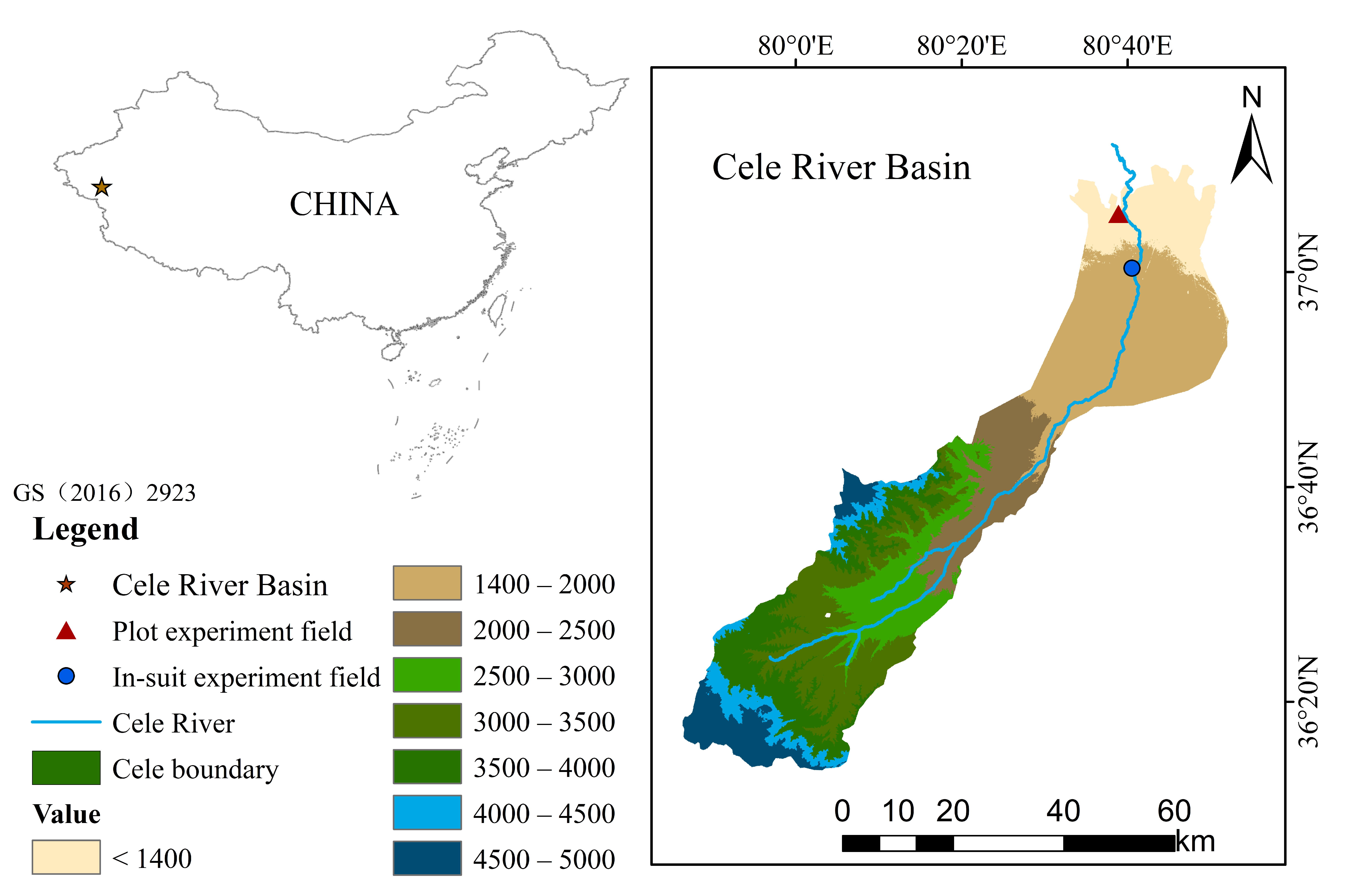
The Cele Oasis is located in the lower reaches of the Cele River on the southern margin of the Tarim Basin, China (35°17′ N–9°30′ N, 80°03′ E–80°10′ E) (Figure 1). The average altitude of the oasis is 1365 m, the length from east to the west is 10 km, and the distance from north to south is 20 km. The glacial meltwater of the Kunlun Mountains constitutes the Cele River, meeting the local water needs. The Cele Oasis is situated in a warm temperate desert climate, with plenty of light, significant temperature differences between day and night, and little rainfall throughout the year. The average annual rainfall in the Cele Oasis is approximately 35 mm and is mainly concentrated between May and August. The multi-year average evaporation is 2500 mm, while the average annual temperature is 11.7 °C.
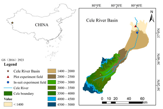
Figure 1.
Location of the study area.
2.2. Experimental Design and Data Introduction
The experiment was divided into two parts: a land plot experiment and a reservoir in-situ experiment. The plot experiment was performed at the National Field Scientific Observation and Research Station of the Cele Desert Grassland Ecosystem in Cele Oasis, the southern margin of the Tarim basin (Figure 1). The land plot experiment is located in the transition zone between the desert and the oasis. The site is open, flat, without shelter, and is well ventilated. Therefore, the site was suitable for evaporation observation experiments. The evaporator was composed of a main evaporation bucket and make-up bucket. According to the FAO standard, the opening of the bucket should be 5–7.5 cm above the ground. However, in this research, due to the large number of small animals such as birds and rabbits, it is difficult to prevent them from drinking the water from the evaporator when the opening of the bucket is 7.5 cm above the ground, resulting in the impact of the experimental data. Therefore, in this research, the opening of the bucket was 10 cm above the ground, the water surface in the evaporation bucket was flush with the ground and the depth of the water was 200 cm. The observation time was 09:00 a.m. every day (Beijing time. The local time is approximately 2 h later than Beijing time). Using the measuring cylinder to fill up the evaporator and records the water volume. The water volume was converted into the depth of the water layer evaporated per unit area of the evaporator, which was the evaporation capacity of that day. The water temperature observation interval of the evaporating dish was one hour. The temperature observations used a PT-100 thermal resistance sensor placed on the water surface (accuracy 0.1 °C). In order to prevent evaporation being affected by floating debris on the water surface, the water surface was regularly cleaned and kept free of obstructions. Since evaporation is directly affected by water temperature, to reduce the impact of changes in water temperature caused by each water replenishment on evaporation, a bucket of water was placed in the experimental field to maintain the water temperature of replenishment as close as possible to the water temperature in the evaporator. The plot experiment began 1 July 2021 and ended at 21 October 2021.
The site of the in-situ experiment in this study was in the XianFeng reservoir, close to the Cele national station. To obtain the evaporation data of the agricultural reservoir, an evaporator was placed 20 m offshore in the reservoir and fixed with a steel frame platform (Figure 2) to keep the evaporator stable. A HOBO water level gauge (U20L-01) was placed at the bottom of the evaporator and 5 cm below the water surface. The HOBO gauge was equipped with a water temperature sensor, which could monitor the water temperature synchronously and had a monitoring interval of 1 h. The reservoir water was added to the evaporator, and the water surface height of evaporator was consistent with that of reservoir. To avoid the influence of salinity in the evaporator on evaporation, water was removed every 3~4 days, and refilled with the reservoir water. Then, the water change in the evaporator was manually measured for comparing and correcting the detection data of the HOBO gauge. The reservoir in-situ experiment was carried out from 6 September to 21 October 2021.
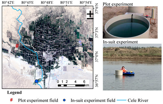
Figure 2.
Locations of plot experiment and in-situ experiment.
The daily average data for various meteorological parameters, such as humidity and wind speed were obtained from the Cele meteorological station. Radiation data were measured using a four-component radiometer with an erection height of 1.5 m.
2.3. Methods
- (1)
- Energy balance method
Based on energy balance theory [10,34], a mathematical model of evaporator evaporation is established to calculate water evaporation. The water–energy balance can be expressed as:
where Rnw is the net radiation at the water surface (W⋅m−2), Hsw is the sensible heat-flux (W⋅m−2), LE is the latent heat-flux (W⋅m−2), Sw is the change in energy stored in the body of water (W⋅m−2), Rs↓ denotes the incoming short-wave radiation(W⋅m−2), αw is the fraction of radiation that penetrates the water surface (αw = 0.087), Rl↓ is the incoming long-wave reflected radiation(W⋅m−2), β is the broadband surface emissivity (β = 0.03), εw is the emissivity of the water body (εw = 0.97), σ is the Stefan–Boltzmann constant, Tw is the water surface temperature (K). The evaporation is converted from the latent heat-flux:
where λ is the latent heat of vaporization (J⋅kg−1) and E is the evaporation rate (mm⋅d−1).
where ρa is the air density (kg⋅m3), cp is the air specific heat capacity (J⋅kg−1⋅K−1), U is the wind speed (m⋅s−1), Ta is the air temperature (K), and CH is the bulk transfer coefficient. CH is calculated as follows:
where qs is the air specific humidity corresponding to the saturated water vapor pressure es with a water surface temperature of Tw, and qa is the air specific humidity corresponding to the air temperature of Ta, qs and qa are calculated as follows:
where es and ea are the saturated water vapor pressure on the water surface and the water vapor pressure at 2 m high, respectively (hPa), and P is the air pressure (hPa), The saturated water vapor pressure on the water surface can be expressed using the water surface temperature Tw:
The change in energy stored in the body of water can be expressed as:
where ρw is the water density (kg⋅m3), cw is the water-specific heat capacity (J⋅kg−1⋅K−1), δz is the depth of the water body (m), and is the rate of change rate of water temperature with time.
- (2)
- Machine learning algorithm
At present, commonly used prediction algorithms mainly include the support vector machine (SVM), regression tree (DT), random forest (RF), cyclic neural network (RNN), and convolutional neural network (CNN) algorithms. In this study, the random forest (RF), least squares support vector machine (LSSVM), long short-term memory network (LSTM), genetic algorithm-back propagation neural network (GA-BP), and convolutional neural network (CNN) algorithms are selected to predict the water surface temperature, and their applicability in terms of water surface temperature prediction are compared.
The random forest (RF) algorithm consists of an ensemble of a large number of classification or regression trees. In RF, each tree grows with a self-serving sample of the original data, and in order to perform the best division, the number of m variables selected randomly by variables is searched [35]. The formation of the classification tree is not dependent on the values of the variables, and the splitting procedure is repeated in each tree until reaching a predefined stop condition [36]. The LSSVM aims to operate on a structural risk minimization principle, where a regularization constraint is placed on the input weights of the mode [37]. This algorithm reduces error and leads to consistent solutions compared with the SVM algorithm. Neural networks are distributed, adaptive, generally nonlinear learning machines that are built from many different nonlinear processing elements called “neurons”, each of which receives connections from other neurons and/or itself according to the training algorithm [38]. The signals flowing on the connections are scaled by adjustable parameters known as weights. In this method, the number of input and output neurons is dependent on the application and is automatically assigned. For the specific details of each machine learning algorithm, see above and these references [36,39,40,41,42,43,44].
- (3)
- Model performance indexes
To compare the difference between the predicted value of the model and the observed value, four indexes are used: the correlation coefficient (r), root mean square error (RMSE), mean absolute error (MAE), and Nash efficiency coefficient (NSE):
where xi is the i-th observation, is the average of the observed values, yi is the i-th value estimated by the model, is the average of the estimated values, and N is the sample size.
3. Results
3.1. Comparison of Evaporation Calculation Results with Observed Values
The water depth of the plain reservoir in the hyper-arid area is shallow and the environment is extremely dry, hot, and windy. Therefore, the water bodies in the upper and lower layers of the reservoir are fully mixed. With shallow water and sufficient agitation, the water body parameters at different depths, such as water temperature, salinity, and velocity, show significant similarity. Therefore, the reservoir water body can be regarded as a uniform temperature state.
The energy balance method is used to calculate the evaporation in the plot experiment and reservoir in-situ experiment. The daily variation and correlation between the calculated values and the observed values of water surface temperature are shown in Figure 3, and the calculation accuracy between the calculated values and the observed values of water surface temperature is shown in Table 1.
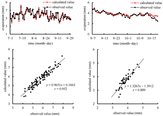
Figure 3.
Dynamic curve and relationship between observed daily evaporation and calculated results (on the left is a comparison between the calculated and observed values of the plot experiment; on the right is a comparison between calculated and observed values in the reservoir in-situ experiment).

Table 1.
Calculation accuracy of energy balance method.
In the plot experiment, the evaporator evaporation value calculated using the energy balance method is close to the observed value (Figure 3), and the change trend between calculated value and observed value is the same, with a good correlation. In the calculation for the reservoir evaporation, the change trend between the observed evaporation and the calculated value is similar, but the fluctuation range of the calculated value is smaller than observed value. The maximum daily evaporation is 4.75 mm, the minimum daily evaporation is 3.24 mm, and the coefficient of variation is 0.08. The observed evaporation varies greatly, and the coefficient of variation is 0.13. In the case of severe evaporation, the observed evaporation value is higher than the calculated evaporation value; in the case of weak evaporation, the observed evaporation value is lower than the calculated evaporation value.
Table 1 shows that the energy balance method performs well in the evaporation calculation of the plot experiment and reservoir in-situ experiment. In the plot experiment, the RMSE between the calculated value and the observed value is 0.337, the MAE is 0.355, the NSE is 0.88, and the r value is as high as 0.952. Compared with the plot experiment, the difference between the calculated value and the observed value in the reservoir in-situ experiment is greater, and the r value is slightly lower, 0.889.
3.2. Analysis of Water Surface Temperature Variation and Relate Influencing Factors
The energy balance method provides a high accuracy in the calculation of water surface evaporation in arid areas. As a critical parameter in the energy balance model, the water surface temperature plays an important role in the accuracy of the evaporation calculation. To accurately simulate changes in the water surface temperature, it is necessary to explore the relationship between the water surface temperature and meteorological factors.
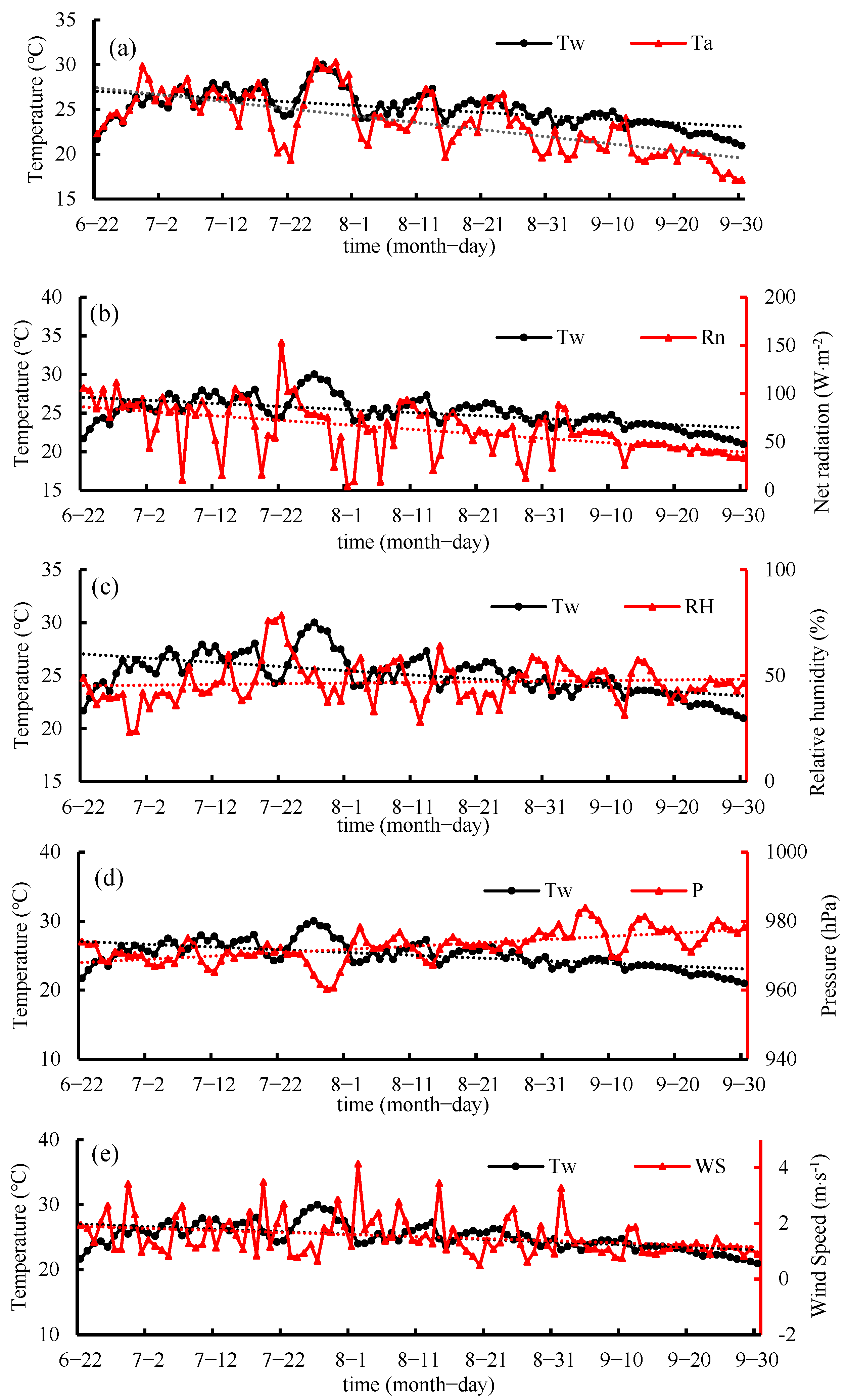
The variations in the water surface temperature (Tw) and air temperature (Ta) over time are shown in Figure 4a. During the observation period, the change trend of the water surface temperature was more consistent with the air temperature, which increases first and then decreases, and their fluctuation laws are similar. Moreover, the fluctuation of the water surface temperature was relatively gentle, but the fluctuation of air temperature was more intense, especially in the period of sudden temperature drop. The change trends of net radiation (Rn) and relative humidity (RH) with time are shown in Figure 4b,c. Over all, the relative humidity showed a downward trend first and then an upward trend, but the change was relatively gentle. The daily average net radiation fluctuated between 4–155 W/m2, which was more violent from July to August, became gentle in the first ten days of September and manifested a negative correlation with humidity in the overall trend. In contrast with the change trend of the wind speed (WS) (Figure 4e), the air pressure (P) experienced a decline first and then rose (Figure 4d). During the observation period, the wind speed fluctuated up and down between 0.4–4.2 m/s with time.

Figure 4.
Variation of water surface temperature and meteorological factors with time (a–e) show the comparison between air temperature, net radiation, relative humidity, air pressure, wind speed and water surface temperature respectively).
According to the above analysis, there is a correlation between the fluctuation pattern of the water surface temperature and meteorological factors. Therefore, a correlation analysis between the water surface temperature and meteorological elements is shown in Table 2. Clearly, the correlation between the water surface temperature and air temperature is the highest, while the correlation between the water surface temperature and wind speed is the lowest.
Table 2.
Correlation between water surface temperature and meteorological factors.
The water surface temperature is greatly affected by the air temperature. The higher the air temperature, the higher the water surface temperature. Moreover, the air pressure and net radiation significantly influence the water surface temperature, but the correlation between the water surface temperature and wind speed is poor.
3.3. Analysis of Machine Learning Water Temperature Prediction Results
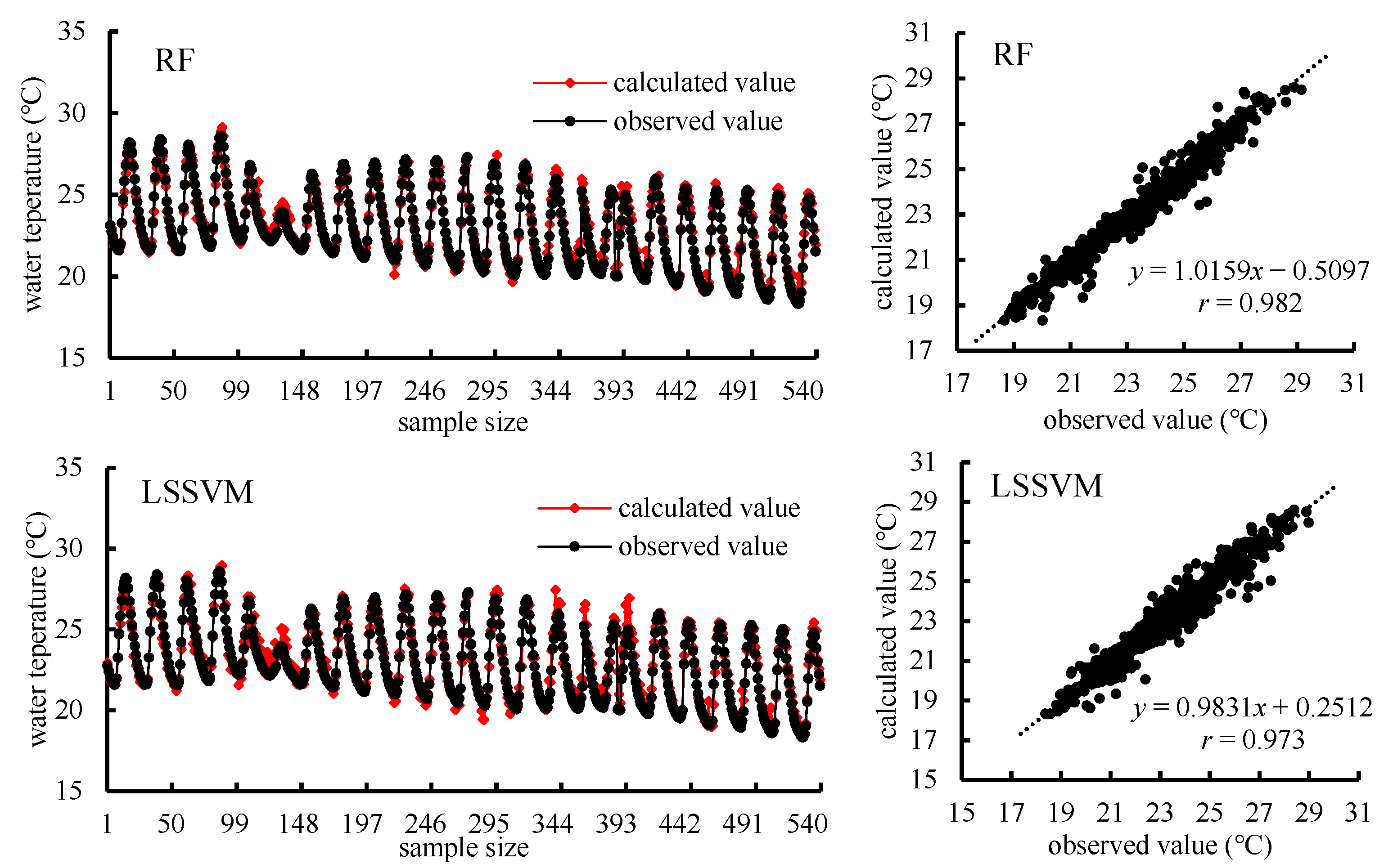
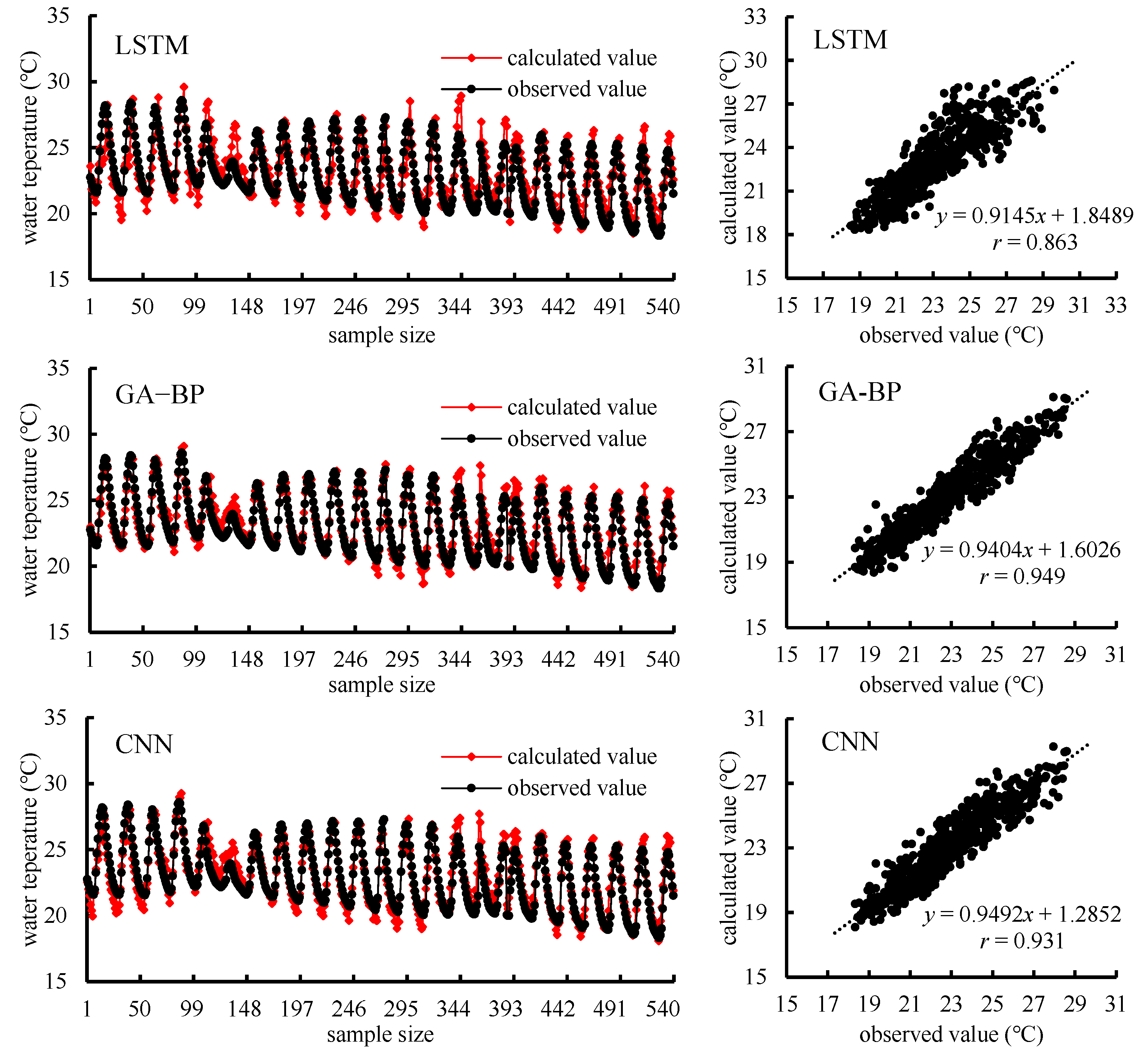
Based on the above research results, the air temperature, air pressure, relative humidity, and net radiation are selected as the algorithm input data, and the hourly water surface temperature is selected as the algorithm output data. When applying the machine learning algorithm, the total sample is divided into a training set sample (accounting for 75% of the total sample) and a verification set sample (remaining samples). With the aid of a correlation analysis between the simulated values and the observed values, the suitability of various algorithms for predicting the water surface temperature are examined. The left side of Figure 5 shows a comparison of hourly simulated and observed values of different machine learning algorithms. The changing trends of the RF and LSSVM algorithms are very similar to the observed values. Compared with the other algorithms, the peak value of the LSTM, GA-BP, and CNN algorithms is higher and the valley value is lower than those of the observed values. On the right side of Figure 5 is a scatter diagram of simulated and observed values corresponding to five machine learning algorithms. Clearly, the r values of the simulated and observed values of all the algorithms are not less than 0.864, indicating that these five machine learning algorithms can be used for short-term water surface temperature prediction.
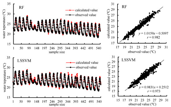
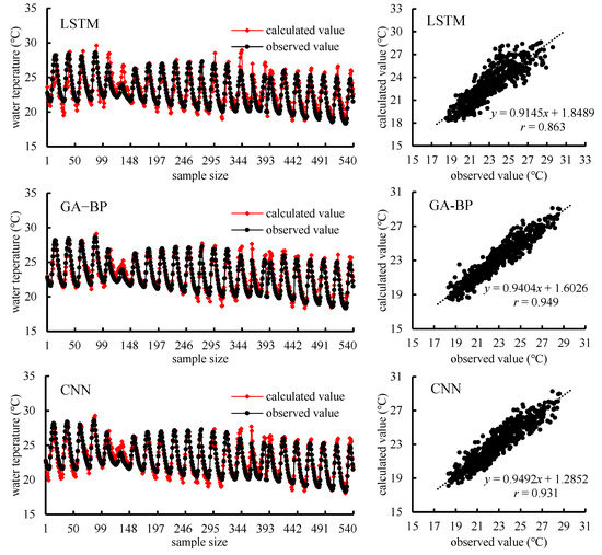
Figure 5.
Dynamic curve and relationship between observed value and calculated value of hourly water temperature.
The r, RMSE, NSE and MAE are used to compare the model simulation results; then, the best machine learning algorithm for water surface temperature prediction in the study area is analyzed.
The statistical indexes related to the prediction results for the five machine learning algorithms (Table 3) reveal that r of the RF algorithm is 0.982, which is higher than that of the other four algorithms. A comparison of the RMSE and MAE values for the five models, i.e., RF (0.464 and 0.336), LSSVM (0.468 and 0.340), LSTM (1.567 and 1.186), GA-BP (0.709 and 0.558), and CNN (1.113 and 0.962), indicate that the RF and LSSVM algorithms perform better than the others with less of a difference between the simulated and observed values. The NSE value of the RF model is 0.968, indicating that this algorithm has a high precision and reliability. The above analysis indicates that the RF algorithm performs best in the prediction of the water surface temperature.
Table 3.
Statistics of fitting results for five machine learning algorithms.
4. Discussion
4.1. Applicability of Energy Balance Method
Agricultural reservoirs in arid areas have shallow water bodies and large areas, and the water surface evaporation is great. Presently, there are no large evaporation tanks with an area of 20 m2 or more available in these areas, and traditional small evaporators are incapable of meeting the requirements of accurate calculations. In this study, an in-situ observation study of land evaporators and reservoirs validates the rationality of the energy balance method. Experimental observation shows that the evaporation of the reservoir is less than that of the land evaporator, which is in line with the research results of others [45,46]. However, there is an error between the reservoir evaporation calculated by the energy balance method and the observed value. This might occur because the evaluation of the energy balance closure of a reservoir system requires accurate estimation of all the energy components in the energy balance method, but there is a lack of surface temperature and soil heat flux data around the reservoir in the in-situ experiment, resulting in a poor closure of the daily energy balance [47]. In this study, the calculation of three parameters (Rnw, Hsw, Sw) in the energy balance method depends on the water surface temperature. One of these is the heat storage of the water body [28,48], which represents the energy stored in the water body as a function of water surface temperature. These parameters (Rnw, Hsw, Sw) will have a significant impact on the closure of the energy balance in the reservoir studied. Since the reservoir was considered as a water body with a uniform temperature in this research, these parameters (Rnw, Hsw, Sw) of the energy balance method are inaccurately calculated, causing some deviation in the results. The calculation error of the water heat storage is the main reason for the calculation error of evaporation. In this study, the shallow water body is regarded as a uniform temperature state. When the heat received from the outside is large and constant, the heat storage in the lower layer of the uniform temperature water body is greater than the actual value, resulting in the reduction of the heat used for evaporation, so the calculated evaporation is less than the observed value. On the contrary, when the heat received from the outside is small and constant, the heat storage in the lower layer of the uniform temperature water body is less than the actual value, resulting in an increase in the heat used for evaporation. Therefore, the calculated evaporation is greater than the observed value. However, in terms of the accuracy indexes (r, RMSE, NSE and MAE), the calculated evaporation is still within an acceptable range, and it can be used to calculate the reservoir water surface evaporation.
4.2. Analysis of Factors Influencing the Water Surface Temperature
The material and energy exchange between water and the atmosphere comprehensively affects the water surface temperature. The factors affecting the water surface temperature mainly include atmospheric forcing, energy distribution, and water surface feedback, in terms of energy balance [49]. These factors are reflected in meteorological elements as temperature, radiation, relative humidity, wind speed, and air pressure. As a result of a change in cloud cover, the solar radiation received by the water surface changes, thereby accelerating or slowing its temperature rise [50,51]. An increase in air temperature and specific humidity also causes a change in water temperature. Many lake studies show that air temperature is the dominant factor in changes in the water surface temperature, and the contribution rate can reach 60% [52]. Changes in the water surface roughness caused by wind speed, alter the heat exchange coefficient between water and air, thus altering the water surface temperature [53,54]. However, in this study, the correlation between the water surface temperature and wind speed is weak, which may be due to the shallow water body and large daily variation in wind speed. After the water body is fully mixed under the influence of wind speed, becoming a uniform temperature water body, the influence of wind speed on water surface temperature is diminished. In addition to being affected by these meteorological factors, the water surface temperature is affected by the characteristics of the water body itself, such as the water level, salinity, water quality [55].
4.3. Main Limitations of the Machine Learning Algorithms
All the machine learning algorithms used in this study can simulate the water surface temperature accurately in a short time sequence. However, except for the cases concerning the RF and LSSVM algorithms, the simulated valley value is lower than the observed value, and the peak value is higher than the observed value in other algorithms. The parameters in the algorithms may need to be further adjusted. Most machine learning algorithms need to use a large number of data and parameters in the process of training and simulation. Too little data or missing values in the data will lead to large error in the simulation results [56]. The set learning time is too long, which sometimes leads to the over fitting of the model, making the simulation results unreliable [57].
Consequently, future research should focus on how to further reduce the amount of input data in the energy balance model, how to accurately simulate water temperature, and how to reduce or eliminate the impact of heat storage terms. In addition, it is not clear whether this method could be applied to the simulation of water surface evaporation in other seasons or other climatic regions due to the short observation time and mainly being concentrated in the summer and autumn of hyper-arid areas. Therefore, more field experiments are needed to verify and improve the model.
5. Conclusions
The energy balance model can satisfactorily simulate the daily variation of evaporator and reservoir evaporation. Under continuous simulation, the RMSE and MAE of the simulated daily evaporation of the evaporator are 0.279 mm/day and 0.245 mm/day, respectively. The correlation coefficient between the daily evaporation simulation values and observed values is 0.946. The RMSE and MAE of the simulated daily evaporation of the reservoir are 0.241 mm/day and 0.257 mm/day, respectively, and the correlation coefficient between the simulated value and the observed value is 0.889.
The main meteorological factors influencing the water surface temperature in the study area, in order of decreasing influence, are air temperature, air pressure, relative humidity, net radiation, and wind speed, of which the water surface temperature is only positively correlated with air temperature, and other meteorological factors are negatively correlated.
In the five machine learning algorithms in this research, the estimation accuracy of the RF model is highest, and its error is the smallest. The RMSE and MAE of the RF model are 0.464 and 0.336, respectively, and the NSE of the RF model is 0.968. That indicates this algorithm has a high reliability and the best applicability of all the models. In general, the RF model, as machine learning algorithm, can be effectively applied to the simulation and prediction of water surface temperature.
These results could not only be used to predict the water surface temperature in the future and to simulate missing data in the past, but also could contribute to the analysis and identification of energy balance. The energy balance model can accurately calculate the water surface evaporation of agricultural reservoirs in hyper-arid areas, and provide a scientific basis for the calculation of a reservoir’s available water and the rational allocation of water resources.
Author Contributions
Conceptualization, C.Y. and D.G.; methodology, C.Y. and Y.L. (Yunfei Liu); Data curation, Y.L. (Yunfei Liu) and W.L.; writing—original draft preparation, C.Y.; writing—review and editing, D.G.; project administration, Y.L. (Yi Liu) and D.G.; funding acquisition, D.G. All authors have read and agreed to the published version of the manuscript.
Funding
This research was funded by National Natural Science Foundation of China, grant number 42171042.
Institutional Review Board Statement
Not applicable.
Informed Consent Statement
Not applicable.
Data Availability Statement
The data presented in this study are available upon request from the corresponding author.
Conflicts of Interest
The authors declare no conflict of interest.
References
- Al-Mukhtar, M. Modeling the monthly pan evaporation rates using artificial intelligence methods: A case study in Iraq. Environ. Earth Sci. 2021, 80, 39. [Google Scholar] [CrossRef]
- Maria Antony Raj, M.; Kalidasa Murugavel, K.; Rajaseenivasan, T.; Srithar, K. A review on flash evaporation desalination. Desalination Water Treat. 2016, 57, 13462–13471. [Google Scholar] [CrossRef]
- Dimitriadou, S.; Nikolakopoulos, K.G. Evapotranspiration Trends and Interactions in Light of the Anthropogenic Footprint and the Climate Crisis: A Review. Hydrology 2021, 8, 163. [Google Scholar] [CrossRef]
- Sun, Z.; Zhu, G.; Zhang, Z.; Xu, Y.; Yong, L.; Wan, Q.; Ma, H.; Sang, L.; Liu, Y. Identifying surface water evaporation loss of inland river basin based on evaporation enrichment model. Hydrol. Processes 2021, 35, e14093. [Google Scholar] [CrossRef]
- Althoff, D.; Rodrigues, L.N.; da Silva, D.D. Evaluating Evaporation Methods for Estimating Small Reservoir Water Surface Evaporation in the Brazilian Savannah. Water 2019, 11, 1942. [Google Scholar] [CrossRef] [Green Version]
- Song, X.P.; Hansen, M.C.; Stehman, S.V.; Potapov, P.V.; Tyukavina, A.; Vermote, E.F.; Townshend, J.R. Global land change from 1982 to 2016. Nature 2018, 560, 639–643. [Google Scholar] [CrossRef]
- Huang, S.; Li, P.; Huang, Q.; Leng, G.; Hou, B.; Ma, L. The propagation from meteorological to hydrological drought and its potential influence factors. J. Hydrol. 2017, 547, 184–195. [Google Scholar] [CrossRef]
- Ogilvie, A.; Riaux, J.; Massuel, S.; Mulligan, M.; Belaud, G.; Le Goulven, P.; Calvez, R. Socio-hydrological drivers of agricultural water use in small reservoirs. Agric. Water Manag. 2019, 218, 17–29. [Google Scholar] [CrossRef]
- Ronco, P.; Zennaro, F.; Torresan, S.; Critto, A.; Santini, M.; Trabucco, A.; Zollo, A.L.; Galluccio, G.; Marcomini, A. A risk assessment framework for irrigated agriculture under climate change. Adv. Water Resour. 2017, 110, 562–578. [Google Scholar] [CrossRef]
- Majidi, M.; Alizadeh, A.; Farid, A.; Vazifedoust, M. Development and application of a new lake evaporation estimation approach based on energy balance. Hydrol. Res. 2018, 49, 1528–1539. [Google Scholar] [CrossRef]
- Majidi, M.; Alizadeh, A.; Farid, A.; Vazifedoust, M. Estimating Evaporation from Lakes and Reservoirs under Limited Data Condition in a Semi-Arid Region. Water Resour. Manag. 2015, 29, 3711–3733. [Google Scholar] [CrossRef]
- Valipour, M.; Sefidkouhi, M.A.G.; Raeini, M. Selecting the best model to estimate potential evapotranspiration with respect to climate change and magnitudes of extreme events. Agric. Water Manag. 2017, 180, 50–60. [Google Scholar] [CrossRef]
- Muhammad, M.K.I.; Nashwan, M.S.; Shahid, S.; Ismail, T.B.; Song, Y.H.; Chung, E.S. Evaluation of Empirical Reference Evapotranspiration Models Using Compromise Programming: A Case Study of Peninsular Malaysia. Sustainability 2019, 11, 4267. [Google Scholar] [CrossRef] [Green Version]
- Pillco Zolá, R.; Bengtsson, L.; Berndtsson, R.; Martí-Cardona, B.; Satgé, F.; Timouk, F.; Bonnet, M.P.; Mollericon, L.; Gamarra, C.; Pasapera, J. Modelling Lake Titicaca’s daily and monthly evaporation. Hydrol. Earth Syst. Sci. 2019, 23, 657–668. [Google Scholar] [CrossRef] [Green Version]
- Schoups, G.; Nasseri, M. GRACEfully Closing the Water Balance: A Data-Driven Probabilistic Approach Applied to River Basins in Iran. Water Resour. Res. 2021, 57, e2020WR029071. [Google Scholar] [CrossRef]
- Jing, W.; Yaseen, Z.M.; Shahid, S.; Saggi, M.K.; Tao, H.; Kisi, O.; Salih, S.Q.; Al-Ansari, N.; Chau, K.W. Implementation of evolutionary computing models for reference evapotranspiration modeling: Short review, assessment and possible future research directions. Eng. Appl. Comput. Fluid Mech. 2019, 13, 811–823. [Google Scholar] [CrossRef] [Green Version]
- Cai, W.; Ullah, S.; Yan, L.; Lin, Y. Remote Sensing of Ecosystem Water Use Efficiency: A Review of Direct and Indirect Estimation Methods. Remote Sens. 2021, 13, 2393. [Google Scholar] [CrossRef]
- Ghiat, I.; Mackey, H.R.; Al-Ansari, T. A Review of Evapotranspiration Measurement Models, Techniques and Methods for Open and Closed Agricultural Field Applications. Water 2021, 13, 2523. [Google Scholar] [CrossRef]
- Kwarteng, E.A.; Gyamfi, C.; Anyemedu, F.O.K.; Adjei, K.A.; Anornu, G.K. Coupling SWAT and bathymetric data in modelling reservoir catchment hydrology. Spat. Inf. Res. 2021, 29, 55–69. [Google Scholar] [CrossRef]
- Song, W.-K.; Chen, Y. Modelling of evaporation from free water surface. Geomech. Eng. 2020, 21, 237–245. [Google Scholar]
- Huth, T.; Hudson, A.M.; Quade, J.; Guoliang, L.; Hucai, Z. Constraints on paleoclimate from 11.5 to 5.0 ka from shoreline dating and hydrologic budget modeling of Baqan Tso, southwestern Tibetan Plateau. Quat. Res. 2015, 83, 80–93. [Google Scholar] [CrossRef]
- Dlouhá, D.; Dubovský, V.; Pospíšil, L. Optimal Calibration of Evaporation Models against Penman-Monteith Equation. Water 2021, 13, 1484. [Google Scholar] [CrossRef]
- Han, S.; Tian, F. Integration of Penman approach with complementary principle for evaporation research. Hydrol. Process. 2018, 32, 3051–3058. [Google Scholar] [CrossRef]
- Vargas Godoy, M.R.; Markonis, Y.; Hanel, M.; Kyselý, J.; Papalexiou, S.M. The Global Water Cycle Budget: A Chronological Review. Surv. Geophys. 2021, 42, 1075–1107. [Google Scholar] [CrossRef]
- Yin, J.; Calabrese, S.; Daly, E.; Porporato, A. The Energy Side of Budyko: Surface-Energy Partitioning From Hydrological Observations. Geophys. Res. Lett. 2019, 46, 7456–7463. [Google Scholar] [CrossRef] [Green Version]
- Sinclair, T.R. “Natural Evaporation from Open Water, Bare Soil and Grass” by Harold L. Penman, Proceedings of the Royal Society of London (1948) A193:120-146. Crop Sci. 2019, 59, 2297–2299. [Google Scholar] [CrossRef]
- Duan, Z.; Bastiaanssen, W.G.M. Evaluation of three energy balance-based evaporation models for estimating monthly evaporation for five lakes using derived heat storage changes from a hysteresis model. Environ. Res. Lett. 2017, 12, 024005. [Google Scholar] [CrossRef] [Green Version]
- Chen, B.; Zuo, H.; Gao, X.; Guo, Y.; Lu, S.; Yang, Y. Study on Pan Evaporation and Energy Change Process by Micro-Meteorological Method. Plateau Meteorol. 2017, 36, 87–97. [Google Scholar]
- Ouellet-Proulx, S.; St-Hilaire, A.; Boucher, M.A. Implication of evaporative loss estimation methods in discharge and water temperature modelling in cool temperate climates. Hydrol. Process. 2019, 33, 2867–2884. [Google Scholar] [CrossRef]
- Yaseen, Z.M.; Al-Juboori, A.M.; Beyaztas, U.; Al-Ansari, N.; Chau, K.W.; Qi, C.; Ali, M.; Salih, S.Q.; Shahid, S. Prediction of evaporation in arid and semi-arid regions: A comparative study using different machine learning models. Eng. Appl. Comput. Fluid Mech. 2020, 14, 70–89. [Google Scholar] [CrossRef] [Green Version]
- Cifuentes, J.; Marulanda, G.; Bello, A.; Reneses, J. Air Temperature Forecasting Using Machine Learning Techniques: A Review. Energies 2020, 13, 4215. [Google Scholar] [CrossRef]
- Ferreira, L.B.; Cunha, F.F.; Silva, G.H.; Campos, F.B.; Dias, S.H.; Santos, J.E. Generalizability of machine learning models and empirical equations for the estimation of reference evapotranspiration from temperature in a semiarid region. An. Acad. Bras. Cienc. 2021, 93, e20200304. [Google Scholar] [CrossRef] [PubMed]
- Bard, N.; Foerster, J.N.; Chandar, S.; Burch, N.; Lanctot, M.; Song, H.F.; Parisotto, E.; Dumoulin, V.; Moitra, S.; Hughes, E.; et al. The Hanabi challenge: A new frontier for AI research. Artif. Intell. 2020, 280, 103216. [Google Scholar] [CrossRef]
- Li, Z.; Pan, N.; He, Y.; Zhang, Q. Evaluating the best evaporation estimate model for free water surface evaporation in hyper-arid regions: A case study in the Ejina basin, northwest China. Environ. Earth Sci. 2016, 75, 295. [Google Scholar] [CrossRef]
- Shabani, S.; Samadianfard, S.; Sattari, M.T.; Mosavi, A.; Shamshirband, S.; Kmet, T.; Várkonyi-Kóczy, A.R. Modeling Pan Evaporation Using Gaussian Process Regression K-Nearest Neighbors Random Forest and Support Vector Machines; Comparative Analysis. Atmosphere 2020, 11, 66. [Google Scholar] [CrossRef] [Green Version]
- Zimmerman, N.; Presto, A.A.; Kumar, S.P.; Gu, J.; Hauryliuk, A.; Robinson, E.S.; Robinson, A.L.; Subramanian, R. A machine learning calibration model using random forests to improve sensor performance for lower-cost air quality monitoring. Atmos. Meas. Tech. 2018, 11, 291–313. [Google Scholar] [CrossRef] [Green Version]
- Kisi, O.; Choubin, B.; Deo, R.C.; Yaseen, Z.M. Incorporating synoptic-scale climate signals for streamflow modelling over the Mediterranean region using machine learning models. Hydrol. Sci. J. 2019, 64, 1240–1252. [Google Scholar] [CrossRef]
- Tezel, G.; Buyukyildiz, M. Monthly evaporation forecasting using artificial neural networks and support vector machines. Theor. Appl. Climatol. 2016, 124, 69–80. [Google Scholar] [CrossRef]
- Ghorbanzadeh, O.; Blaschke, T.; Gholamnia, K.; Meena, S.R.; Tiede, D.; Aryal, J. Evaluation of Different Machine Learning Methods and Deep-Learning Convolutional Neural Networks for Landslide Detection. Remote Sens. 2019, 11, 196. [Google Scholar] [CrossRef] [Green Version]
- Naghibi, S.A.; Ahmadi, K.; Daneshi, A.A. Application of Support Vector Machine, Random Forest, and Genetic Algorithm Optimized Random Forest Models in Groundwater Potential Mapping. Water Resour. Manag. 2017, 31, 2761–2775. [Google Scholar] [CrossRef]
- Alom, M.Z.; Taha, T.M.; Yakopcic, C.; Westberg, S.; Sidike, P.; Nasrin, M.S.; Hasan, M.; Van Essen, B.C.; Awwal, A.A.; Asari, V.K. A State-of-the-Art Survey on Deep Learning Theory and Architectures. Electronics 2019, 8, 292. [Google Scholar] [CrossRef] [Green Version]
- Wu, Y.; Yuan, M.; Dong, S.; Lin, L.; Liu, Y. Remaining useful life estimation of engineered systems using vanilla LSTM neural networks. Neurocomputing 2018, 275, 167–179. [Google Scholar] [CrossRef]
- Ahmadi, M.H.; Ahmadi, M.A.; Nazari, M.A.; Mahian, O.; Ghasempour, R. A proposed model to predict thermal conductivity ratio of Al2O3/EG nanofluid by applying least squares support vector machine (LSSVM) and genetic algorithm as a connectionist approach. J. Therm. Anal. Calorim. 2019, 135, 271–281. [Google Scholar] [CrossRef]
- Deo, R.C.; Kisi, O.; Singh, V.P. Drought forecasting in eastern Australia using multivariate adaptive regression spline, least square support vector machine and M5Tree model. Atmos. Res. 2017, 184, 149–175. [Google Scholar] [CrossRef] [Green Version]
- De Farias Mesquita, J.B.; Neto, I.E.L.; Raabe, A.; de Araújo, J.C. The influence of hydroclimatic conditions and water quality on evaporation rates of a tropical lake. J. Hydrol. 2020, 590, 125456. [Google Scholar] [CrossRef]
- Rodrigues, C.M.; Moreira, M.; Guimarães, R.C.; Potes, M. Reservoir evaporation in a Mediterranean climate: Comparing direct methods in Alqueva Reservoir, Portugal. Hydrol. Earth Sci. 2020, 24, 5973–5984. [Google Scholar] [CrossRef]
- Tanny, J.; Cohen, S.; Assouline, S.; Lange, F.; Grava, A.; Berger, D.; Teltch, B.; Parlange, M.B. Evaporation from a small water reservoir: Direct measurements and estimates. J. Hydrol. 2008, 351, 218–229. [Google Scholar] [CrossRef] [Green Version]
- Lensky, N.G.; Dvorkin, Y.; Lyakhovsky, V.; Gertman, I.; Gavrieli, I. Water, salt, and energy balances of the Dead Sea. Water Resour. Res. 2005, 41, 1–13. [Google Scholar] [CrossRef]
- Tan, Z.; Yao, H.; Zhuang, Q. A Small Temperate Lake in the 21st Century: Dynamics of Water Temperature, Ice Phenology, Dissolved Oxygen, and Chlorophyll a. Water Resour. Res. 2018, 54, 4681–4699. [Google Scholar] [CrossRef]
- Yang, K.; Yu, Z.; Luo, Y.; Zhou, X.; Shang, C. Spatial-Temporal Variation of Lake Surface Water Temperature and Its Driving Factors in Yunnan-Guizhou Plateau. Water Resour. Res. 2019, 55, 4688–4703. [Google Scholar] [CrossRef]
- Gooseff, M.N.; Strzepek, K.; Chapra, S.C. Modeling the potential effects of climate change on water temperature downstream of a shallow reservoir, Lower Madison River, MT. Clim. Change 2005, 68, 331–353. [Google Scholar] [CrossRef]
- Schmid, M.; Köster, O. Excess warming of a Central European lake driven by solar brightening. Water Resour. Res. 2016, 52, 8103–8116. [Google Scholar] [CrossRef]
- Hatmaja, R.B.; Wisha, U.J.; Radjawane, I.M.; Al Tanto, T. Correlation and coherence analysis between sea surface temperature (SST) and surface wind in the Equatorial Western Sumatra Waters. In Proceedings of the 1st International Conference On Tropical Meteorology and Atmospheric Sciences (ICTMAS), Bandung, Indonesia, 19–20 September 2018. [Google Scholar]
- Koue, J.; Shimadera, H.; Matsuo, T.; Kondo, A. Numerical Analysis of Sensitivity of Structure of the Stratification in Lake Biwa, Japan by Changing Meteorological Elements. Water 2018, 10, 1492. [Google Scholar] [CrossRef] [Green Version]
- Biazar, S.M.; Fard, A.F.; Singh, V.P.; Dinpashoh, Y.; Majnooni-Heris, A. Estimation of evaporation from saline water. Environ. Monit. Assess. 2020, 192, 694. [Google Scholar] [CrossRef]
- Ding, S.; Zhao, H.; Zhang, Y.; Xu, X.; Nie, R. Extreme learning machine: Algorithm, theory and applications. Artif. Intell. Rev. 2015, 44, 103–115. [Google Scholar] [CrossRef]
- Wang, P.; Zheng, X.; Ku, J.; Wang, C. Multiple-Instance Learning Approach via Bayesian Extreme Learning Machine. IEEE Access 2020, 8, 62458–62470. [Google Scholar] [CrossRef]


Publisher’s Note: MDPI stays neutral with regard to jurisdictional claims in published maps and institutional affiliations. |
© 2022 by the authors. Licensee MDPI, Basel, Switzerland. This article is an open access article distributed under the terms and conditions of the Creative Commons Attribution (CC BY) license (https://creativecommons.org/licenses/by/4.0/).