A Deep Learning-Based Model to Reduce Costs and Increase Productivity in the Case of Small Datasets: A Case Study in Cotton Cultivation

Abstract

In this paper, a deep-learning model is proposed as a viable approach to optimize the information on soil parameters and agricultural variables’ effect in cotton cultivation, even in the case of small datasets. In this study, soil is analyzed to reduce the planting costs by determining the various combinations of soil components and nutrients’ precise amounts. Such factors are essential for cotton cultivation, since their amounts are often not precisely defined, and especially traditional farming methods are characterized by excessive distribution volumes producing significant economic and environmental impact. Not only can artificial intelligence decrease the charges, but it also increases productivity and profits. For this purpose, a deep learning algorithm was selected among other machine learning algorithms by comparison based on the accuracy metric to build the predictive model. This model gets the combination of the factors amounts as input and predicts whether the cotton growth will be successful or not. The predictive model was built by this algorithm based on 13 physical and chemical factors has 98.8% accuracy.

1. Introduction

Machine learning (ML) is a technique widely implemented for finding patterns and linear and non-linear relationships between different variables. From the statistic point of view, a model is counted as linear if the model’s parameters are linear [1]. ML has various subcategories such as Classification, Regression, or Clustering, which can be utilized in order to analyze and to help make decisions [2]. Machine learning is gaining an increasing interest in agriculture, where complex relationships often have to be investigated to solve complex agri-engineering problems [3]. On the other hand, agricultural practices suffer from the availability of a reduced amount of data and information on the many relevant parameters. Among others, soil organic matter (SOM) and pH are critical factors regarding the degradation that might occur due to unsuitable management practices [4]. For preventing such occurrence and to predict the accuracy of prediction in terms of SOM, Yang et al. [5] employed four different machine learning approaches, namely: partial least squares regression (PLSR), least squares-support vector machines (LS-SVM), extreme learning machines (ELM), and cubist regression model (Cubist). Ashapure et al. [6] took advantage of the Machine learning method to estimate the yield of planted crops. Three features were utilized for the scope: multi-temporal features, non-temporal features, and irrigation status. The machine learning algorithm was based on an artificial neural network (ANN), and two other algorithms named support vector regression (SVR) and random forest regression (RFR) were employed and compared with ANN: ultimately the ANN model outperformed the other ones. Osco et al. [7] utilized ML algorithms applied to maize images in order to build a regression model, which can help increase corn productivity by estimating the nitrogen and plant height. Parent et al. [8] used machine learning to make decisions, which can help crop fertilization and soil conservation methods.

As mentioned, many factors are influential in agriculture and especially in cotton planting, which is used as a case study in this paper. Therefore, knowing the impact of different factors on crop yields and the actual value of each factor is of importance in order to optimize field production. As highlighted by literature, one of the state-of-the-art methods to achieve such a goal is through the adoption of machine learning algorithms [9]. Papageorgiou et al. [10] utilized the machine learning algorithm as a decision support system in order to predict the crop yield and improve crop management. Schuster et al. [11] was aimed at finding the best suited area for cotton cultivation, and for this goal, applied k-means machine learning as a functional method to identify and choose the management zones. In the reported research, two sets of attributes were utilized (crop yield and field slope and conductivity), and the application of the ML algorithm allowed identification of the optimal zones for cotton growth. Hong et al. [12] examined 257 soil samples in order to determine which elements in the soil can directly correlate to the organic matter in rice and cotton cultivations. In order to enhance the accuracy of the information, he applied extreme learning machine (ELM), which is a feedforward neural network where the parameters of hidden nodes do not need to be adjusted, and support vector machine (SVM) were applied, wavebands were utilized as input. Consequently, both algorithms could measure the organic matter, although the former was more accurate than the latter.

1.1. Cotton

Cotton is known as the most valuable non-food crop. Cotton products generate revenue for more than 250 million people worldwide. This outstanding crop is functional in different areas, making currency and paper, cooking oil, animal feed packaging, and biofuels [13]. The importance of cotton can be examined from different perspectives. One of the most outstanding values of cotton is its undeniably direct impact on the economy of a country: it is expected that the cotton market value will grow, from $38.54 billion in 2020 to $46.56 billion in 2027. Therefore, this industry’s consumption, production, export, and imports are expected to increase rapidly [14].

In the cotton industry, the feasibility of cotton harvesting mainly depends on the characteristics of the soil in which the cotton is planted. Soil components such as salinity, gravimetric water content, or bulk density can positively affect cotton growth and quality [15]. Although traditional farming methods are still employed in some regions, artificial intelligence can be utilized to decrease costs and increase productivity in product planting and harvesting.

Many factors have been analyzed in cotton cultivation, and research results can highly improve the cotton planting process. Sadras et al. stated that environmental factors such as the duration of the season or average humidity could affect the cotton yield [16]. Bakhsh et al. suggested that the most critical factors in cotton cultivation must include plant protection, fertilizers, and land preparation [17]. Braunack described the components that can directly correlate to the cotton-growing known as a cultivator, growing region, the amount of nitrogen and phosphorus in the soil, the amount of rainfall, season length, and the appropriate date for defoliation [18]. Besides the environmental effect, the row space is crucial in this field due to boll weevil; hence, considering the space can markedly affect the crops. If it is not considered due to lack of experience, the farmer may lose many crops [19].

In addition to other factors, it was concluded that the quality of the soil where cotton is grown is highly significant in cotton crop growth [20]. Hulugalle et al. studied soil nutrients and resiliency in terms of growing cotton [21]. During three different periods, the effect of various factors on cotton growth was investigated by the authors, and soil pH, electrical conductivity, and moisture were required to be concentrated on as the most crucial elements [21]. The presence of substances such as calcium (Ca), magnesium (Mg), potassium (K), sodium (Na), and nitrate-Nitrogen (N) indicates the fertility area for planting cotton. Ouattara conducted research by examining the effects of rainfall on the cotton-growing, and he verified that rainfall is a fundamental contributing factor in cotton fiber yields [22]. After doing considerable research, Gemtos et al. identified Mg as an essential soil factor for growing high-quality cotton [23,24].

Ali et al. pointed out the factors that can have adverse effects on cotton yields; among others, high temperature, greenhouse gas emission, drought stress, salinity stress, insects, or pests attack were selected as the underlying factors to be considered in cotton growth [25]. Therefore, farmers and stakeholders should take soil related factors into consideration in order to generate high-quality cotton to be used in various industries. Furthermore, such information might be iterated on a relatively long time scale in order to overcome variability due to weather or ascribable to other time-dependent sources [26,27].

1.2. Soil Characteristics Effect on Cotton Cultivation

Soil nutrient content impacts cotton planting efficiency and growth. For instance, nitrogen is recommended in the range of 90 to 140 kg/ha. Moreover, the multiple phases in the agricultural process and the impact of the ecosystem’s dynamic changes might alter soil parameters and its nutrient content. For this reason, the availability and number of elements should be monitored and adjusted [28]. Consequently, based on these reasons, the relative costs might be increased. Machine learning methods can be thus employed in order to predict soil nutrient substances to decrease the fertilizer cost and raise profits, and this prediction also optimizes the working time and enhances soil health [29].

In this paper, soil, one of the significant factors in cotton cultivation, is analyzed with the aim of decreasing the charges by specifying the various combinations of soil components and nutrients’ precise amounts. For this purpose, machine learning and deep learning algorithms are employed, eventually making a predictive model based on independent variables. Such independent variables, like pH, temperature, humidity, density, electrical conductivity, grain surface, nitrogen, phosphorus, calcium, particle spacing, potassium, and magnesium are the ones that are essential for cotton cultivation but are often prone to uncertainty and excessive applications in the traditional farming methods, with a negative impact on costs as well as on the environment. Not only can artificial intelligence reduce expenses, but it also increases productivity and profits by supporting the farmers in their management decisions. The lower are cultivation costs, the higher will be the investment in improving the quality of prerequisites for planting and harvesting. This predictive model is aimed at supporting farmers to practically reach the proper combination of factors for growing cotton with the lowest costs. This is achieved:

• considering and analyzing 13 essential factors in soil for cotton planting.
• utilizing artificial intelligence methods for reducing costs and increasing productivity and profits in cotton cultivation.
• solving uncertainty for selecting the factors amounts.

The remainders of the paper are organized as follows. Section 2 describes machine learning and deep learning algorithms and the other methods utilized for preprocessing and evaluation. In Section 3, experimental results are presented. Section 4 expresses the conclusion.

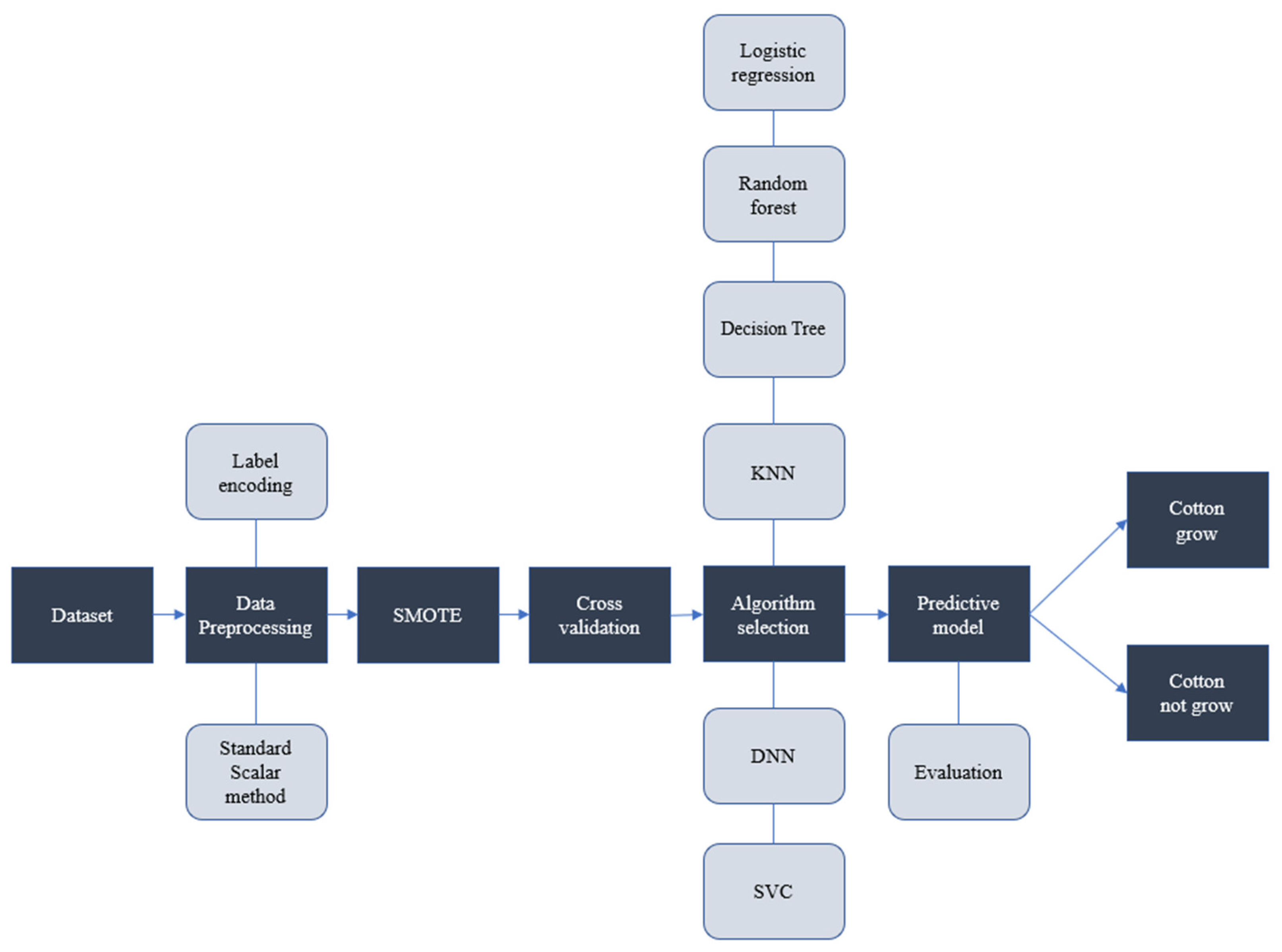
2. Materials and Methods

In this section, the machine learning and deep learning processes, which are utilized to build the predictive model, are briefly described. The Synthetic Minority Oversampling Technique is presented, as a method used for preprocessing steps in imbalanced datasets. A method to validate the predictive model, the K-fold cross-validation, is eventually described.

2.1. Machine Learning

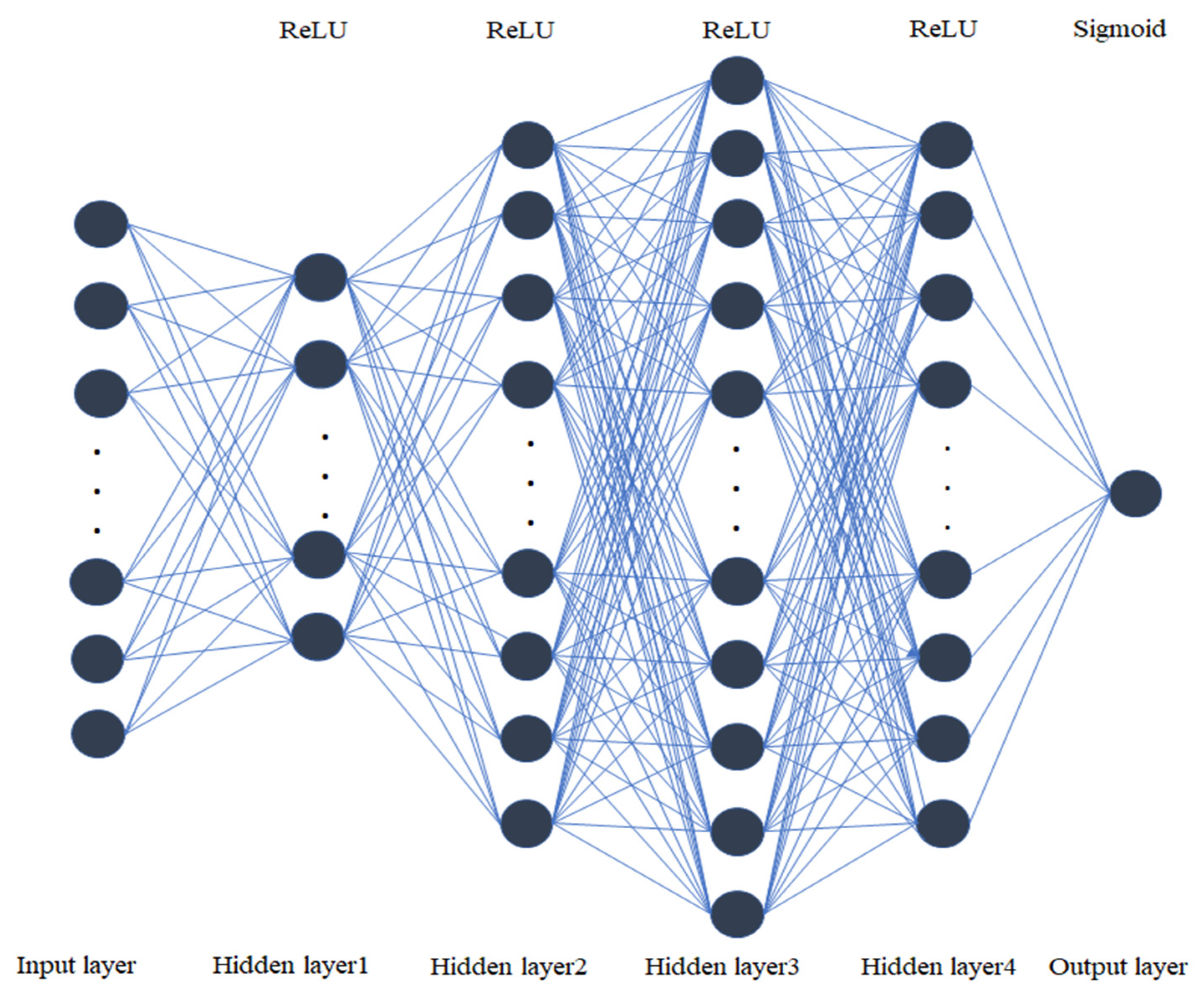
The classification method aims to build a predictive model that can opportunely process and organize a set of input data into specific classes. Figure 1 illustrates the classification process, in which Synthetic Minority Oversampling Technique (SMOTE) is utilized to solve the imbalanced dataset problem, and the logistic regression, random forest, decision tree, k-nearest neighbors (KNN), and support vector classifier (SVC) are used to build the classifier.

Deep learning is a subset of machine learning algorithms characterized by various architectures, including deep neural networks (DNNs), convolutional neural networks (CNNs), recurrent neural networks (RNNs), etc.

2.2. Deep Learning

A deep neural network is utilized to build the predictive model. DNN is an artificial neural network (ANN) algorithm with several hidden layers [30,31]. The proposed DNN model in this paper has four hidden layers. Figure 2 provides a graphical representation of the proposed DNN schema.

The DNN model is created with Stochastic Gradient Descent (SGD) in seven steps:

• the weights are initialized with small values randomly (i.e., values close to 0);
• each feature is placed in one input node in the input layer;
• Forward-Propagation operation is applied: the neurons from the input layer to the output layer are activated so that the weights limit each neuron’s activation; such operation proceeds until convergence is reached on y prediction.
• the error is calculated by comparing the prediction and actual value;
• in this step, a backpropagation operation is exerted: the weights are updated based on how much they are relevant for the error, while the learning rate value determines the weight update.
• steps 1 to 5 are repeated, but the weights are updated after Batch learning;
• when the process is done, an epoch is completed: more epochs are done to train a better model.

Each layer has its own bias and weights, and each layer’s calculation and applying activation function is mentioned in Equations (1)–(5):

$$h_i^{\left(1\right)}=f^{\left(1\right)} ({\displaystyle \sum }_j{w}_{ij}^{\left(1\right)} X_j+b_i^{\left(1\right)})$$

(1)

$$h_i^{\left(2\right)}=f^{\left(2\right)} ({\displaystyle \sum }_j{w}_{ij}^{\left(2\right)} h_j^{\left(1\right)}+b_i^{\left(2\right)})$$

(2)

$$h_i^{\left(3\right)}=f^{\left(3\right)} ({\displaystyle \sum }_j{w}_{ij}^{\left(3\right)} h_j^{\left(2\right)}+b_i^{\left(3\right)})$$

(3)

$$h_i^{\left(4\right)}=f^{\left(4\right)} ({\displaystyle \sum }_j{w}_{ij}^{\left(4\right)} h_j^{\left(3\right)}+b_i^{\left(4\right)})$$

(4)

$$y_i=f^{\left(5\right)} ({\displaystyle \sum }_j{w}_{ij}^{\left(5\right)} h_j^{\left(4\right)}+b_i^{\left(5\right)})$$

(5)

where y_i is the prediction, w indicates the weight, h_i^(N) are units in the N-th hidden layer, f is the activation function, X_j represents the input observations. The rectified linear unit (ReLU) is utilized for four hidden layers as an activation function, which is formulated in agreement with Equation (6):

$$f \left(X\right)=max \left(0,X\right)$$

(6)

The problem in this paper is a binary classification; therefore, the sigmoid function is employed as an activation function for the output layer. The sigmoid function is formulated as reported in Equation (7):

$$f \left(X\right)=\frac{1}{1+e^{-X}}$$

(7)

The backpropagation is applied to adjust the weights for minimizing the loss function. This operation compares the probability of the actual value and the probability of the prediction value to minimize cost function and improve the DNN model performance. The cost function considered in this model is the Cross-entropy function, which is formulated as follows (8).

$$Cost=-\frac{1}{m}{\displaystyle \sum }_{i=1}\left[ {\overline{y}}_i log \left(y_i\right)+\left(1-{\overline{y}}_i\right) log \left(1-y_i\right)\right]$$

(8)

Several optimization algorithms were developed based on the SGD algorithm, such as adaptive gradient algorithm (AdaGrad), adaptive moment estimation (Adam), root means square propagation (RMSProp). In other words, these algorithms are extensions of the SGD algorithm.

Adam is an optimization algorithm that can be counted as a combination of AdaGrad and RMSProp algorithms [32]. Adam takes advantage of both algorithms, which utilize the moving average of the gradient like AdaGrad and implements the squared gradients to scale the learning rate like RMSProp. Adam updates the weights in a way formulated in Equation (9).

$$\begin{gathered} m_{t+1}\leftarrow {\beta }_1{m}_t+\left(1-{\beta }_1\right) \nabla C_t \\ {v}_{t+1}\leftarrow {\beta }_2{v}_t+\left(1-{\beta }_2\right) {\left(\nabla C_t\right)}^2 \\ \widehat{m}=\frac{m_{t+1}}{1-{\beta }_1^{t+1}} \\ \widehat{v}=\frac{v_{t+1}}{1-{\beta }_2^{t+1}} \\ {w}_{t+1} \leftarrow w_t-\eta \frac{\widehat{m}}{\sqrt{\widehat{v} }+ϵ} \end{gathered}$$

(9)

where w is model weight, m is the first moment (i.e., m is mean), v is the second moment (i.e., v is uncentered variance), C is the cost function, β₁ and β₂ are hyperparameters, ϵ is a small scalar, and η is the learning rate (step size). The hyperparameters will be optimized by the GridSearch method.

2.3. Data Standardization and Label-Encoding Technique

The factors considered as independent variables to build the predictive model are reported in

Table 1. The independent variables for cotton grow prediction.

Variable	Type	Value	Role
pH	Numerical	Range of numbers	Independent
Temperature	Numerical	Range of numbers	Independent
Humidity	Numerical	Range of numbers	Independent
Density	Numerical	Range of numbers	Independent
Electrical conductivity	Numerical	Range of numbers	Independent
Grain Surface	Categorical	Smooth, Scaly, Gritty, Fibrous	Independent
Nitrogen (N)	Numerical	Range of numbers	Independent
Phosphorus (P)	Numerical	Range of numbers	Independent
Calcium (Ca)	Numerical	Range of numbers	Independent
Particle Spacing	Categorical	Close, Crowded	Independent
Potassium (K)	Numerical	Range of numbers	Independent
Magnesium (Mg)	Numerical	Range of numbers	Independent
Particle Width	Categorical	Narrow, Broad	Independent
Cotton grows	Categorical	Yes (1), No (0)	Dependent

.

In a dataset with independent variables not in the same range, the features that exhibit larger variance than others maybe dominate the target and make the algorithm impotent to learn appropriately from other independent variables. The StandardScalar method is utilized to avoid such limitations [33]: the problem is solved by standardizing the independent variables (i.e., the mean is removed, and unit variance is scaled for independent variables). The operation is formulated in Equation (10), where s is the standard deviation, and μ is the mean.

$$Z=\frac{X-\mu }{S}$$

(10)

Based on Table 1, there are three categorical independent variables. These features should be converted into numerical features; accordingly, the Label-encoding or OneHot-encoding techniques should be utilized to solve this problem. There are several categories in each categorical feature: for this reason, OneHote-encoding might be not a good choice due to the generation of many columns and to the increased complexity in the analysis process. Therefore, the Label-encoding technique, which handles the categorical variables by assigning a unique integer to each label, was preferred in this paper.

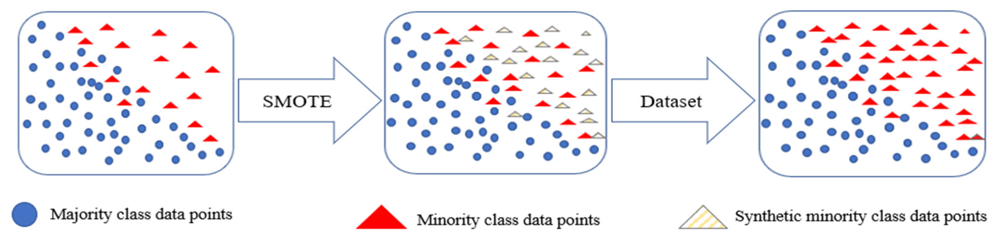
2.4. Synthetic Minority Oversampling Technique

There are too few samples of the minority class in the dataset; therefore, the predictive model cannot adequately learn the decision boundary: the SMOTE is utilized to solve this problem as described in [34].

In this technique, a random sample from the minority class is selected, and the K number of the nearest neighbors is determined for that sample. One of the neighbors is picked randomly, and a synthetic sample is made at a randomly chosen point between the two samples in feature space. This process is repeated to produce enough samples for the minority class. Figure 3 illustrates the SMOTE process.

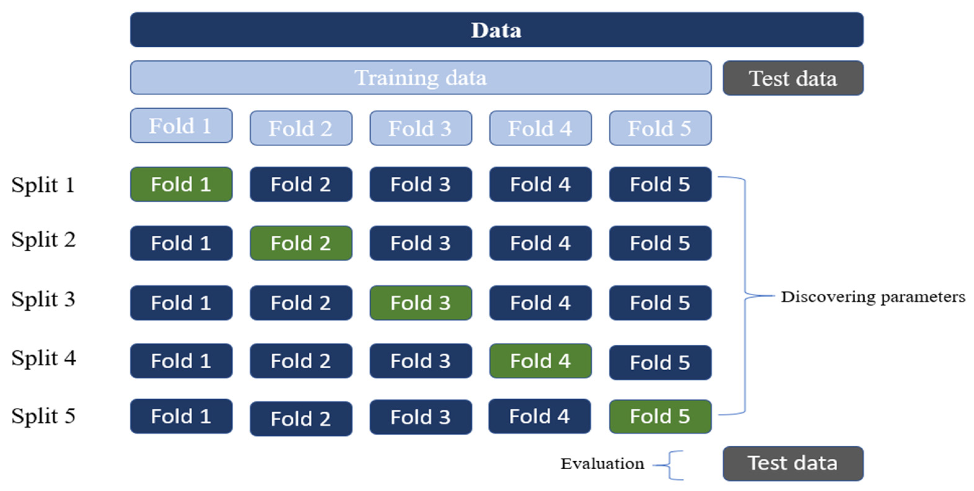
2.5. K-Fold Cross-Validation

K-fold cross-validation is exerting to small datasets to avoid overfitting (i.e., the machine learning model has adequately learned but cannot converge to an appropriate prediction). In this statistical method, the training set is apportioned into K smaller sections; subsequently, the machine learning model is prepared by using K-1 of the units, and the remaining section is utilized for the validation. This process repeats, and each time the training units and validation section change, the test part is used for the final assessment; consequently, the average of accuracies is calculated. Figure 4 shows the K-fold cross-validation process.

2.6. Performance Evaluation Metrics

There are several methods commonly applied to evaluate the performance of the classification model, such as Precision, Recall, F1-score, and Accuracy. The Precision, Recall, F1-score, and Accuracy metrics are calculated based on Equations (11)–(14).

$$\mathrm{Precision} =\frac{\mathrm{TP}}{\mathrm{TP} + \mathrm{FP}}$$

(11)

$$\mathrm{Recall} =\frac{\mathrm{TP}}{\mathrm{TP} + \mathrm{FN}}$$

(12)

$$\mathrm{Accuracy} =\frac{\mathrm{TP} + \mathrm{TN}}{\mathrm{TP} + \mathrm{TN} + \mathrm{FP} + \mathrm{FN}}$$

(13)

$$\mathrm{F}1-\mathrm{score} =\frac{\mathrm{TP}}{\mathrm{TP} +\frac{1}{2}\left(\mathrm{FP} + \mathrm{FN}\right)}$$

(14)

where TP, TN, FP, and FN are described as follows:

−

True Positive (TP): the predictive model predicted is positive, and the primary value is positive;

−

True Negative (TN): the predictive model is predicted negative, and the primary value is negative;

−

False Positive (FP): the predictive model is predicted positive, but the primary value is negative (Type 1 error);

−

False Negative (FN): the predictive model is predicted negative, but the primary value is positive (Type 2 error).

2.7. Confidence Interval

The confidence interval is a statistical method that is implemented to quantify and determine the uncertainty of a prediction. This method can interpret the predictive model’s skill and prepare a more robust model. The size of the confidence interval determines the precision of the estimation. Choosing a smaller confidence interval brings a more precise estimate. The radius of the confidence interval for the model’s accuracy and error can be calculated by Equation (15).

$$\begin{gathered} I=Z\times \sqrt{\frac{A\times \left(1-A\right)}{n}} \\ I=Z\times \sqrt{\frac{e\times \left(1-e\right)}{n}} \end{gathered}$$

(15)

where I is the radius of the confidence interval, n is the sample size, e is the error, A is accuracy, and Z is the standard deviation value from the gaussian distribution.

3. Results and Discussion

In this section, the best algorithm for building the predictive model among machine learning and deep learning algorithms is chosen by comparison based on the accuracy metric. Subsequently, the evaluation metrics are utilized to assess the results. Tensorflow package is employed to implement the deep learning algorithm, and the Scikit-learn package is used for machine learning algorithms; Python 3.7 is utilized to implement and run the algorithms.

3.1. Preprocessing and Hyperparameter Tuning

Before the predictive model is built, two operations are carried out in preprocessing step. Firstly, the Label encoding technique is used to convert the categorical features into numerical ones. Secondly, the StandardScalar method improves the predictive model performance by removing each independent variable’s mean and adjusting them to unit variance based on the formula introduced in Equation (10). Based on Figure 5, one of the classes has less sample (12%); therefore, the SMOTE technique is utilized to solve the imbalanced dataset problem.

There are various hyperparameters in the DNN classification model, which can increase the model performance by tuning the hyperparameters themselves. The GridSearch method is here utilized for this goal. The adjusted hyperparameters by the GridSearch method are reported in

Table 2. The adjusted hyperparameters.

No	Hyperparameter	Value
1	Layers size	(7, 36, 50, 30, 1)
2	Optimizer	Adam
3	Batch size	10
4	Epoche	100

.

3.2. Comparison of DNN with Other Machine Learning Algorithms and Model Evaluation

In this step, the DNN algorithm is compared with several classification algorithms, namely logistic regression, Support vector classifier, K-nearest neighbors (KNN), random forest regression, and decision tree based on the accuracy metric. The algorithms comparison is reported in

Table 3. The algorithms comparison.

No	Algorithm	Accuracy (%)
1	Support vector classifier (kernel: RBF, gamma: scale)	92.1
2	Logistic regression (penalty: l2)	93.2
3	Decision tree (criterion: gini, max depth: nodes are expanded until all leaves pure)	88.5
4	KNN (number of neighbors: 5)	89.3
5	Random forest (number of trees: 100)	92
6	DNN	98.8

.

According to the results reported in Table 3, the DNN algorithm has the best performance (98.8%): thus, it was selected as the algorithm to build the predictive model in the present paper. The K-fold cross-validation technique was utilized to avoid overfitting problems and to get a robust performance for the predictive model. The DNN model’s predictions based on a few test data samples are denoted in

Table 4. The DNN model prediction.

Instance	DNN Model
	Feature (pH, T *, H *, D *, EC *, N *, P *, K *, Ca *, Mg *, GS *, PS *, PW *)	Prediction Class	Actual Class
1	(6.5, 20.8, 82, 0.92, 7.4, 100, 50, 43, 30, 19, 3, 0, 1)	0	0
2	(7.03, 21.77, 80.31, 1.04, 1.35, 85, 58, 41, 12.25, 5.15, 3, 0, 0)	0	0
3	(6.93, 26.1, 71.57, 1.52, 6.16, 129, 44, 27, 18.74, 11.16, 1, 1, 0)	1	1
4	(5.97, 18.47, 62.69, 1.54, 6.45, 101, 38, 40, 34.73, 16.91, 1, 1, 0)	0	1
5	(6.65, 23.55, 71.59, 1.47, 5.2, 95, 43, 36, 27.49, 19.16, 1, 1, 0)	1	1
6	(6.92, 19.02, 17.13, 1.42, 9.21, 23, 72, 84, 6.61, 9.76, 2, 0, 0)	0	0
7	(7.23, 24.4, 79.19, 1.4, 6.15, 133, 47, 34, 45.86, 11.14, 1, 1, 0)	1	1
8	(6.82, 24.88, 75.62, 1.5, 5.76, 134, 47, 53, 42.9, 23.76, 1, 1, 0)	1	1
9	(6.82, 28.17, 81.04, 0.78, 2.2, 10, 56, 16, 11.39, 7.55, 1, 1, 0)	1	1
10	(7.03, 28.33, 80.77, 1.51, 11.57, 8, 54, 20, 5.66, 8.84, 3, 1, 1)	0	0

* Note: T = Temperature, H = Humidity, D = Density, EC = Electrical, Conductivity, N = Nitrogen, P = Phosphorus, K = Potassium, Ca = Calcium, Mg = Magnesium, GS = Grain Surface, PS = Particle Spacing, PW = Particle Width.

.

The Precision, Recall, F1-score are implemented in order to evaluate the predictive model: the results are denoted for each class in

Table 5. The evaluation result.

Class		Metrics
	Precision (%)	Recall (%)	F1-Score (%)
0	98	99	98
1	100	98	99

.

The confidence interval radius is calculated through Equation (15) for the DNN model to get a more reliable result. There are four common significance levels, which can be selected to get more robust predictions. The outcome is reported in

Table 6. The confidence interval radius.

Significance Level (%)	Z	Radius (%)	Accuracy Range (%)
90	1.64	$\pm$1.9	(96.9, 100)
95	1.96	$\pm$2.3	(96.5, 100)
98	2.33	$\pm$2.5	(96.3, 100)
99	2.58	$\pm$2.8	(96, 100)

.

3.3. Discussion

In the previous studies, a part of influential factors in cotton cultivation was considered in each research. For instance, some researchers only worked on pH, electrical conductivity, and moisture; others investigated other factors such as nutrients in the soil needed for cotton cultivation or other environmental factors [16,17,18,19,20,21,22,23,24,25,26,27,28]. Moreover, some studies employed artificial intelligence methods in other sections of cotton or other crops planting and harvesting as, for instance, cotton or other crops yield prediction, identification of the proper area for planting, evaluation of appropriate temperature for crop growth based on imagery data, or detection of cotton leaf diseases. On the other hand, the present study, not only introduces a novel technique such as deep learning to reach an appropriate analysis in the cotton cultivation and fertilization process, leading to increase the productivity and reduce costs but also takes into consideration 13 effective factors (both physical and chemical ones) in order to reach a practical and more comprehensive model and analysis.

This research provided a DNN algorithm, which is selected among other machine learning algorithms based on a comparison of the accuracy to build a classifier that can determine the proper amount of soil parameters in the cotton cultivation process. In the preprocessing step, due to the existence of the categorical variables, heterogeneity of features ranges, and the problem of imbalance dataset, the label-encoding, standard-scalar, and SMOTE techniques were employed to solve the issues, respectively. The DNN algorithm was selected among other machine learning algorithms due to its better performance to build the classifier, which results were mentioned in Table 3. For a quantitative evaluation, three common metrics, namely, precision, recall, and F1-score, were specifically implemented: the resulting values are reported in Table 5. Additionally, since cotton cultivation is a sensitive process, the confidence interval method was used to take more robust and trustable results (see Table 6).

There are various expenses in the planting and harvesting of the cotton crop, one of which is fertilization costs. Due to the uncertainty in determining the amount of soil chemical and physical parameters, which are necessary for cotton cultivation, the fertilization costs might increase. In agreement with the recommendations of digital farming, by utilizing new technology such as the proposed DNN model, the farmers and decision-makers can determine the factors amounts with a higher level of accuracy and accordingly decrease the fertilization costs by reaching an appropriate combination of factors. The same approach might be implemented whenever small datasets are available, and an optimized model is needed in order to improve the effectiveness, efficiency, and sustainability of input resources.

4. Conclusions

This paper was aimed to discuss the application of artificial intelligence in agriculture, even in the common case of small available datasets. The approach was applied and verified in the specific case of cotton cultivation to allow a reduction of expenses and increase profits and yield. A predictive model was built by the DNN algorithm with 98.8% accuracy based on 13 essential factors that are soil parameters and its nutrient content. This model receives the combination of the amounts of the elements as input and predicts whether the cotton growth will be successful or not. Therefore, the uncertainty problem for choosing the factors amounts have been solved; consequently, the planting costs decrease, and the yield and profits rise. For future research, other new technology such as IoT can be integrated with artificial intelligence, and different deep learning algorithms and techniques can be considered to increase the model performance.

References

1. Amani, M.A.; Ebrahimi, F.; Dabbagh, A.; Rastgoo, A. A machine learning-based model for the estimation of the temperature-dependent moduli of graphene oxide reinforced nanocomposites and its application in a thermally affected buckling analysis. Eng. Comput. 2021, 37, 2245–2255. [Google Scholar] [CrossRef]
2. Behdinian, A.; Amani, M.A.; Aghsami, A.; Jolai, F. An integrating Machine learning algorithm and simulation method for improving Software Project Management: A real case study. J. Qual. Eng. Prod. Optim. 2022; in press. [Google Scholar] [CrossRef]
3. Recchia, L.; Boncinelli, P.; Cini, E.; Vieri, M.; Pegna, F.G.; Sarri, D. Multicriteria Analysis and LCA Techniques: With Applications to Agro-Engineering Problems. Green Energy Technol. 2017, 142, 248–259. [Google Scholar]
4. Obalum, S.; Chibuike, G.U.; Peth, S.; Ouyang, Y. Soil organic matter as sole indicator of soil degradation. Environ. Monit. Assess. 2017, 189, 176. [Google Scholar] [CrossRef]
5. Yang, M.; Xu, D.; Chen, S.; Li, H.; Shi, Z. Evaluation of machine learning approaches to predict soil organic matter and pH using Vis-NIR spectra. Sensors 2019, 19, 263. [Google Scholar] [CrossRef] [Green Version]
6. Ashapure, A.; Jung, J.; Chang, A.; Oh, S.; Yeom, J.; Maeda, M.; Maeda, A.; Dube, N.; Landivar, J.; Hague, S.; et al. Developing a machine learning based cotton yield estimation framework using multi-temporal UAS data. ISPRS J. Photogramm. Remote Sens. 2020, 169, 180–194. [Google Scholar] [CrossRef]
7. Osco, L.P.; Junior, J.M.; Ramos, A.P.M.; Furuya, D.E.G.; Santana, D.C.; Teodoro, L.P.R.; Gonçalves, W.N.; Baio, F.H.R.; Pistori, H.; Junior, C.A.S.; et al. Leaf nitrogen concentration and plant height prediction for maize using UAV-based multispectral imagery and machine learning techniques. Remote. Sens. 2020, 12, 3237. [Google Scholar] [CrossRef]
8. Parent, L.E.; Natale, W.; Brunetto, G. Machine Learning, Compositional and Fractal Models to Diagnose Soil Quality and Plant Nutrition. In Soil Science—Emerging Technologies, Global Perspectives and Applications; IntechOpen: London, UK, 2021. [Google Scholar]
9. Li, Y.; Chao, X. Ann-based continual classification in agriculture. Agriculture 2020, 10, 178. [Google Scholar] [CrossRef]
10. Papageorgiou, E.I.; Markinos, A.T.; Gemtos, T.A. Fuzzy cognitive map based approach for predicting yield in cotton crop production as a basis for decision support system in precision agriculture application. Appl. Soft Comput. 2011, 11, 3643–3657. [Google Scholar] [CrossRef]
11. Schuster, E.W.; Kumar, S.; Sarma, S.E.; Willers, J.L.; Milliken, G.A. Infrastructure for Data-Driven Agriculture: Identifying Management Zones for Cotton Using Statistical Modeling and Machine Learning Techniques. In Proceedings of the 8th International Conference & Expo on Emerging Technologies for a Smarter World, Hauppauge, NY, USA, 2–3 November 2011; pp. 1–6. [Google Scholar]
12. Hong, Y.; Chen, S.; Zhang, Y.; Chen, Y.; Yu, L.; Liu, Y.; Liu, Y.; Cheng, H.; Liu, Y. Rapid identification of soil organic matter level via visible and near-infrared spectroscopy: Effects of two-dimensional correlation coefficient and extreme learning machine. Sci. Total Environ. 2018, 644, 1232–1243. [Google Scholar] [CrossRef]
13. Fabric. The Fabric of Our Lives. 2020. Available online: https://thefabricofourlives.com/the-benefits-of-cotton (accessed on 8 December 2021).
14. Texprocil Ibtex News Clippings. Ibtex No.26. 2021. Available online: https://texprocil.org/IBTEXNewsClippings.htm (accessed on 8 December 2021).
15. Corwin, D.; Lesch, S.; Shouse, P.; Soppe, R.; Ayars, J.E. Identifying soil properties that influence cotton yield using soil sampling directed by apparent soil electrical conductivity. Agron. J. 2003, 95, 352–364. [Google Scholar] [CrossRef] [Green Version]
16. Sadras, V.; Bange, M.; Milroy, S. Reproductive allocation of cotton in response to plant and environmental factors. Ann. Bot. 1997, 80, 75–81. [Google Scholar] [CrossRef] [Green Version]
17. Bakhsh, K.; Hassan, I.; Maqbool, A. Factors affecting cotton yield: A case study of Sargodha (Pakistan). J. Agric. Soc. Sci. 2005, 1, 332–334. [Google Scholar]
18. Braunack, M. Cotton farming systems in Australia: Factors contributing to changed yield and fibre quality. Crop Pasture Sci. 2013, 64, 834–844. [Google Scholar] [CrossRef]
19. Paim, E.A.; Dias, A.M.; Showler, A.T.; Campos, K.L.; Castro Grillo, P.P.; Bastos, C.S. Cotton row spacing for boll weevil management in low-input production systems. Crop Prot. 2021, 145, 105614. [Google Scholar] [CrossRef]
20. Chen, W.; Jin, M.; Ferré, T.P.; Liu, Y. Soil conditions affect cotton root distribution and cotton yield under mulched drip irrigation. Field Crop. Res. 2020, 249, 107743. [Google Scholar] [CrossRef]
21. Hulugalle, N.; Nehl, D.; Weaver, T.B. Soil properties, and cotton growth, yield and fibre quality in three cotton-based cropping systems. Soil Tillage Res. 2004, 75, 131–141. [Google Scholar] [CrossRef]
22. Ouattara, K. Improved Soil and Water Conservatory Managements for Cotton-Maize Rotation System in the Western Cotton Area Of Burkina Faso. Ph.D. Thesis, Swedish University of Agricultural Sciences, Uppsala, Sweden, 2007. [Google Scholar]
23. Gemtos, T.; Markinos, A.; Nassiou, T. Cotton lint quality spatial variability and correlation with soil properties and yield. Precis. Agric. 2005, 5, 361–368. [Google Scholar]
24. Tan, L.; Zhang, Y.; Marek, G.W.; Ale, S.; Brauer, D.K.; Chen, Y. Modeling basin-scale impacts of cultivation practices on cotton yield and water conservation under various hydroclimatic regimes. Agriculture 2022, 12, 17. [Google Scholar] [CrossRef]
25. Ali, M.A.; Ilyas, F.; Danish, S.; Mustafa, G.; Ahmed, N.; Hussain, S.; Arshad, M.; Ahmad, S. Soil Management and Tillage Practices for Growing Cotton Crop. In Cotton Production and Uses; Springer: Berlin/Heidelberg, Germany; Singapore, 2020; pp. 9–30. [Google Scholar]
26. Kayad, A.; Sozzi, M.; Gatto, S.; Whelan, B.; Sartori, L.; Marinello, F. Ten years of corn yield dynamics at field scale under digital agriculture solutions: A case study from North Italy. Comput. Electron. Agric. 2021, 185, 106126. [Google Scholar] [CrossRef]
27. Pluto-Kossakowska, J. Review on multitemporal classification methods of satellite images for crop and arable land recognition. Agriculture 2021, 11, 999. [Google Scholar] [CrossRef]
28. Sozzi, M.; Kayad, A.; Gobbo, S.; Cogato, A.; Sartori, L.; Marinello, F. Economic comparison of satellite, plane and uav-acquired NDVI images for site-specific nitrogen application: Observations from Italy. Agronomy 2022, 11, 2098. [Google Scholar] [CrossRef]
29. Pezzuolo, A.; Basso, B.; Marinello, F.; Sartori, L. Using SALUS model for medium and long term simulations of energy efficiency in different tillage systems. Appl. Math. Sci. 2014, 8, 6433–6445. [Google Scholar] [CrossRef]
30. Alfian, G.; Syafrudin, M.; Fitriyani, N.L.; Anshari, M.; Stasa, P.; Svub, J.; Rhee, J. Deep Neural Network for Predicting Diabetic Retinopathy from Risk Factors. Mathematics 2021, 8, 1620. [Google Scholar] [CrossRef]
31. Sozzi, M.; Cantalamessa, S.; Cogato, A.; Kayad, A.; Marinello, F. Automatic bunch detection in white grape varieties using YOLOv3, YOLOv4, and YOLOv5 deep learning algorithms. Agronomy 2022, 12, 319. [Google Scholar] [CrossRef]
32. Kingma, D.P.; Ba, J. Adam: A method for stochastic optimization. arXiv 2014, arXiv:1412.6980. [Google Scholar]
33. Hale, J. Scale, Standardize, or Normalize with Scikit-Learn. 2019. Available online: https://towardsdatascience.com/scale-standardize-or-normalize-with-scikit-learn-6ccc7d176a02 (accessed on 8 December 2021).
34. Chawla, N.V.; Bowyer, K.W.; Hall, L.O.; Kegelmeyer, W.P. SMOTE: Synthetic minority over-sampling technique. J. Artif. Intell. Res. 2002, 16, 321–357. [Google Scholar] [CrossRef]
Figure 1. The Classification process.
Agriculture 12 00267 g001
Figure 2. The proposed DNN schema.
Agriculture 12 00267 g002
Figure 3. The SMOTE process.
Agriculture 12 00267 g003
Figure 4. K-fold cross-validation process.
Agriculture 12 00267 g004
Figure 5. Each class label percentage.
Agriculture 12 00267 g005