Characteristics of Potential Evapotranspiration Changes and Its Climatic Causes in Heilongjiang Province from 1960 to 2019

Abstract

Climate change refers to the statistically significant changes in the mean and dispersion values of meteorological factors. Characterizing potential evapotranspiration (ET₀) and its climatic causes will contribute to the estimation of the atmospheric water cycle under climate change. In this study, based on daily meteorological data from 26 meteorological stations in Heilongjiang Province from 1960 to 2019, ET₀ was calculated by the Penman–Monteith formula, linear regression method and the Mann–Kendall trend test were used to reveal the seasonal and inter-annual changing trend of ET₀. The sensitivity-contribution rate method was used to clarify the climatic factors affecting ET₀. The results showed that: (1) From 1960 to 2019, the maximum temperature (T_max), minimum temperature (T_min) and average temperature (T_mean) showed an increasing trend, with climate tendency rate of 0.22 °C per decade (10a), 0.49 °C/(10a), 0.36 °C/(10a), respectively. The relative humidity (RH), wind speed (U) and net radiation (Rn) showed a decreasing trend, with a climate tendency rate of −0.42%/(10a), −0.18 m/s/(10a), −0.08 MJ/m²/(10a), respectively. (2) ET₀ showed a decreasing trend on seasonal and inter-annual scales. Inter-annually, the average climate tendency rate of ET₀ was −8.69 mm/(10a). seasonally, the lowest climate tendency rate was −6.33 mm/(10a) in spring. (3) ET₀ was negatively sensitive to T_min, and RH, while positively sensitive to T_max, T_mean U and Rn, its sensitivity coefficient of U was the highest, which was 1.22. (4) The contribution rate of U to ET₀ was the highest on an inter-annual scale as well as in spring and autumn, which were −8.96%, −9.79% and −13.14%, respectively, and the highest contribution rate to ET₀ were Rn and T_min in summer and winter, whose contribution rates were −4.37% and −11.46%, respectively. This study provides an understanding on the response of evapotranspiration to climatic change and further provides support on the optimal allocation of regional water resource and agricultural water management under climate change.

1. Introduction

Over the past 100 years (1906–2005), the global average surface temperature has increased by 0.74 °C and is expected to increase by at least 4 °C in 2100 if carbon dioxide emissions are not reduced [1]. Climate change will inevitably lead to changes in the global hydrological cycle [2]. Apart from precipitation and runoff, actual evapotranspiration (ET) is the most important climatic factor and a main component in the hydrological cycle [3]. Evapotranspiration is affected by a variety of meteorological factors, such as temperature, relative humidity (RH), wind speed (U), and net radiation (Rn). Characteristics of ET changes and its climatic causes under climate change will reveal the water cycle process and its driving mechanism.

Due to the complexity of the ET process, it is difficult to directly measure the ET: however, with the deepening of vegetation ET research, obtaining regional continuous ET data by calculating the ET becomes particularly vital. Potential evapotranspiration (ET₀), as the basis for calculating the ET [4], represents the maximum ET that can be achieved on a fixed underlying surface with unlimited water supply under certain meteorological conditions. ET₀ is widely used in the analysis of climate dry and wet conditions, rational use and evaluation of water resources, crop water demand and agricultural production management, and ecological environment research [5]. There are many ways to calculate ET₀, such as temperature and the solar radiation-based Hargreaves method, the equilibrium evaporation-based Priestley-Taylor model and the FAO Blaney–Criddle formula [6]. However, many scholars choose the Penman-Monteith method recommended by the FAO56 to calculate ET₀. The advantage of the Penman–Monteith method is that standard meteorological data are easily obtained or obtained through routine observation, and all calculation procedures can be standardized by the calculation of available meteorological data and time scales [7].

ET₀ was heterogeneous in temporal and spatial distribution. Jung et al. [8] pointed out that the global average annual ET increased at a rate of 7.1 ± 1.0 mm/10a from 1982 to 1997, but since 1998, the global average ET decreased by −7.9 mm/10a. Roderick et al. [9] found that in the past 50 years, the ET₀ in the northern hemisphere was decreasing at a faster rate of 2 to 4 mm/a. ET₀ also showed an increasing trend in some areas, such as West Africa [10] and Turkey [11]. Wu et al. [12] pointed out that the national annual average ET₀ decreased at a rate of 0.52 mm/a based on the daily meteorological data of 552 meteorological stations in China from 1961 to 2015, and the ET₀ of most stations in arid and humid regions showed a significant decreasing trend; however, neither the increasing nor decreasing trend of ET₀ is significant in semi-arid and semi-humid regions. The decrease or increase of ET₀ may affect the hydrological cycle differently. For example, when the ET₀ decreases, the transport of water vapor in the atmosphere is reduced, resulting in corresponding changes in precipitation patterns. For agriculture, the water use efficiency of crops may be improved by reducing the adverse effects of drought on crops. However, the increase of ET₀ will increase water consumption, resulting in increased land water loss and drought, and the atmospheric circulation may be affected, which may lead to strong rainfall, thus changing the distribution of water resources.

The spatio–temporal heterogeneity of ET₀ was attributed to the common effect of different climatic factors, including maximum temperature (T_max), minimum temperature (T_min), average temperature (T_mean), RH, U and sunshine hours, while the dominant factors affecting ET₀ varied in different regions. For example, Bandyopadhyay et al. [13] concluded that the main reason for the decrease of ET₀ in India was the significant increase in RH and decrease of U by the non-parametric method of Sen’s slope. Roderick et al. [14] believed that the decrease in solar radiation caused by the increase in cloud cover and aerosol concentration in the southern hemisphere was the main reason for the decrease of ET₀ in New Zealand. Hossein et al. [15] believed that U has the greatest impact on ET₀ in Iranian region under arid climate condition by sensitivity analysis. Guo et al. [16] used the Sobol global sensitivity analysis method to analyze the sensitivity of ET₀ in Australia calculated by the Penman–Monteith and Priestley–Taylor models and obtained that air temperature was the most sensitive factor to ET₀. China has seven geographic regions, with complex and diverse climatic characteristics. ET₀ has shown a fluctuating downward trend in recent decades, such as Henan Province in Central China [17], Anhui Province in East China [18], Sichuan Basin [19] and Huaihe basin [20] in Southwest China; the results of the sensitivity-contribution rate method showed that the contribution of U to ET₀ was higher than that of sunshine hours, indicating that U was the dominant meteorological factor in the above area. On the contrary, in North China, the results of the sensitivity coefficient method showed that sunshine hours were the dominant factor, followed by U [21]. Zhou et al. [22] analyzed the partial correlation between ET₀ and meteorological factors by discussing climate attribution and concluded that the increase of the T_max in the Three River Headwaters region located in Northwest China was the main reason for the increasing trend of ET₀, however, the contribution of U was the smallest among all meteorological factors, which was different from the meteorological factors affecting the trend of ET₀ in other regions.

Heilongjiang Province, located in one of the four major black soil belts in the world, has an existing land area of 454,600 km² and an area of 23,900 km² of arable land. It is the largest province in terms of grain production in the country. In recent years, Heilongjiang Province has become one of the regions with the largest temperature rise in the country and one of the regions with more serious climate disasters, threatening the safe production of food crops. The impact of floods and droughts on the agricultural economy in Heilongjiang Province accounted for about 89.4% of the total impact of various natural disasters [23]; the reduction of grain production due to floods and droughts accounted for about 12% of the total grain output in the same period [24]. Nie et al. [25] speculated that the climate in Heilongjiang Province would continue to warm in the next 30 and 50 years, and water resources would be scarcer. The probability of drought is increasing. ET₀, as a key factor to characterize the regional dry and wet conditions, is of great significance for guiding water resource management and agricultural production management in Heilongjiang Province. Jiang et al. [26] expounded on the various characteristics of ET₀ in Heilongjiang Province from the scale of the crop growing season and pointed out that ET₀ was the most sensitive to RH, which provided an important reference index for formulating a reasonable irrigation system for the crop growing season in Heilongjiang Province. However, their study was limited to the growing season of crops, which could not fully reflect the changes of ET₀ in Heilongjiang Province between inter-annual and different seasons; moreover, contributing rates of different climate factors were not analyzed. Su et al. [27] pointed out that the contribution rate of water vapor pressure and U to the ET₀ change in Heilongjiang Province was the largest by multiple regression analysis, and it has a certain significance for understanding the influencing factors on the inter-annual change of ET₀. However, they failed to study the impact of more meteorological factors on a shorter time scale. The weather of Heilongjiang Province changes significantly in four seasons, and ET₀ may be affected by different climatic factors in seasonal scales.

This study used a linear regression equation and the Mann–Kendall method to analyze the trend of ET₀ in Heilongjiang Province in the past 60 years on the inter-annual and seasonal scales. The sensitivity coefficient and contribution of different climate factors to ET₀ were comprehensively analyzed by the sensitivity-contribution rate method, aiming to provide an important basis for the rational and efficient use of water resources and agricultural water management in different regions of Heilongjiang Province under climate change.

2. Materials and Methods

2.1. Overview of the Study Area and Data Sources

Heilongjiang Province, located in the east of Eurasia, is the northernmost province with the highest latitude in China, starting at 121°11′ in the west, 135°05′ in the east, 43°26′ in the south, and 53°33′ in the north, spanning 14 longitudes from east to west and 10 latitudes from north to south, with an average altitude of 481 m. It has a temperate continental monsoon climate. It spans the four major river systems of the Heilongjiang River, Wusuli River, Songhua River and Suifenhe River. The average annual temperature of Heilongjiang Province is between −5 and 5 °C, gradually increasing from the north to the south. The annual precipitation is between 400 and 650 mm, with more in the central mountainous areas, followed by the east, and less in the west and north. The annual sunshine hours in the province are mostly between 2400 and 2800 h, where the west is more than the east.

The meteorological data in this study were from the daily meteorological data of 26 meteorological stations (Figure 1) in Heilongjiang Province from 1960 to 2019 recorded by the China Meteorological Data Network, including T_max, T_min, T_mean, RH, U, and sunshine hours; Rn was calculated according to the method recommended by the Food and Agriculture Organization of the United Nations (FAO) [7]. According to the meteorological division method, March to May is divided into spring, June to August is summer, September to November is autumn, and December to February is winter [28].

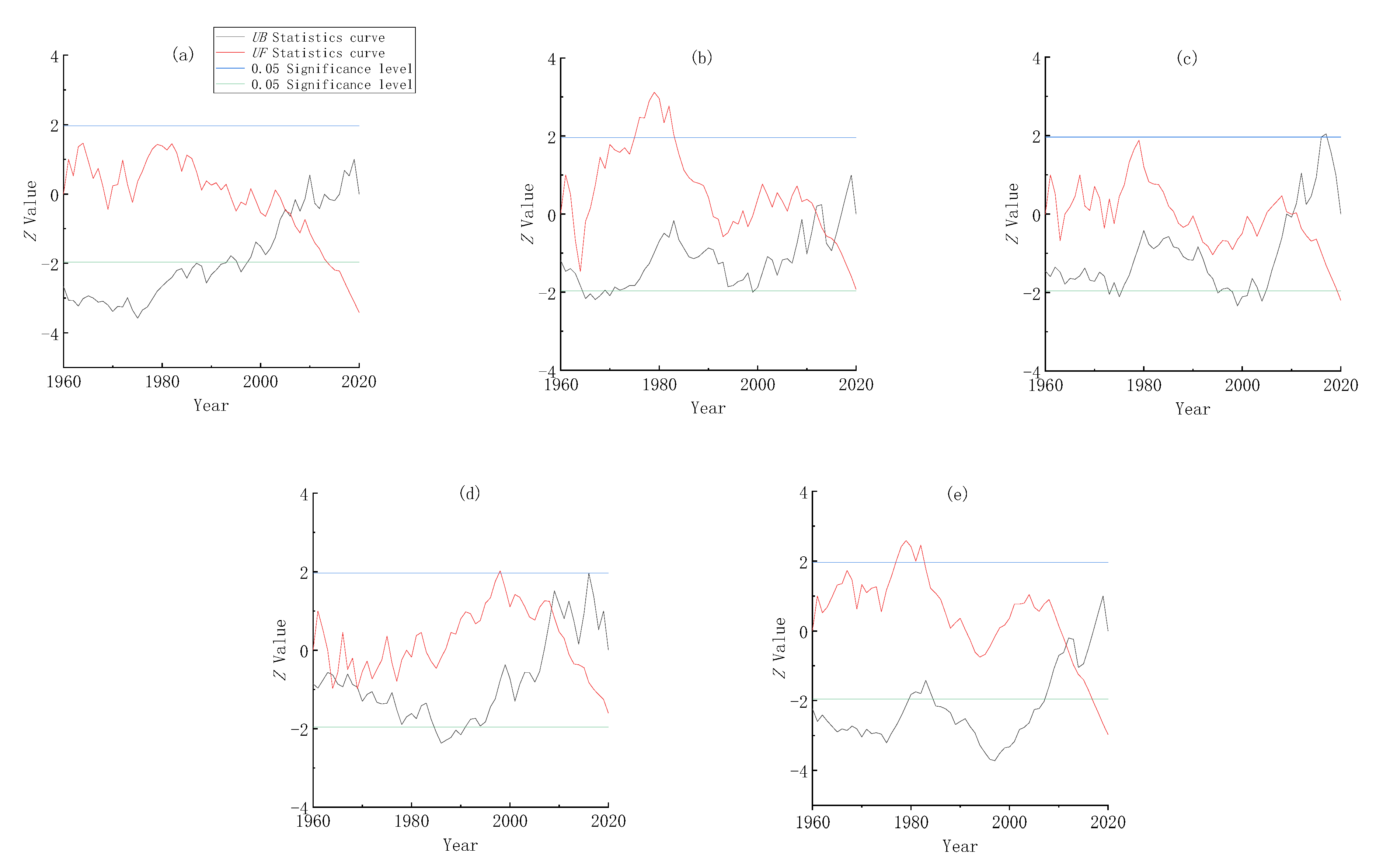
2.2. Mann–Kendall Trend and Mutation Test

For the time series X, (containing n samples), an order column is constructed:

$$S_k={\displaystyle \sum }_{i=1}^k{r}_i \left(k=2, 3, \dots , n\right)$$

(1)

where

$$r_i=\{ \begin{array}{c}+1 x_i>x_j\\ 0 or\end{array} \left(\mathrm{j}=1, 2,\dots , i\right)$$

(2)

The order column S_k is the sum of the number of values when the value of the i moment is greater than the j moment.

Under the assumption that the time series is random, define the statistic:

$$U{F}_k=\frac{\left[S_k-E\left(S_k\right)\right]}{\sqrt{Var\left(S_k\right)}} \left(\mathrm{k}=1, 2,\dots , n\right)$$

(3)

where UF₁ = 0, E(S_k) and Var(S_k) are the mean and variance of S_k, respectively, and when X₁, X₂,…, X_n are independent of one other, they have the same continuous distribution, which can be deduced from the following equation:

$$E\left(S_k\right)=\frac{n\left(n+1\right)}{4}, Var\left(S_k\right)=\frac{n\left(n-1\right)\left(2n+5\right)}{72}(2\le \mathrm{k}\le n)$$

(4)

UF_k is a standard normal distribution, it is a sequence of statistics calculated in the order of time series X (X₁, X₂,…, X_n); given the significance level α by checking the normal distribution table, if UF_i > U_α, it indicates that there is a significant trend change in the sequence. Then repeat the above process in the reverse order of time series X (X_n, X_n−1,…, X₁) and make UB_k = UF_k (k = n, n−1, …, 1), UB₁ =0.

Generally, if the significance level α = 0.05, then the critical value Z = ±1.96. The curves of the two statistical sequences of UF, UB and the two straight lines of ±1.96 are plotted on one plot. If the values of UF and UB are greater than 0, it indicates an upward trend in the series, and if the values of UF and UB are less than 0, it indicates a downtrend. When UF and UB exceed the critical line, it indicates a significant upward or downward trend, and the range above the critical line is determined as the time zone in which the mutation occurred. If the two curves of UF and UB intersect and the intersection point is between the critical lines, then the moment corresponding to the intersection point is the time when the mutation begins [29].

2.3. Climate Tendency Rate

The climate tendency rate was calculated by the least squares method, and the unary linear regression equation of Y_i and X_i was established:

Y_i = AX_i + B

(5)

where A and B are regression constants, and A × 10 is the climate tendency rate, representing the changing rate of each climatic factor every 10 years (10a). A positive value indicates an increasing trend of climate in the corresponding time series, while a negative value indicates a decreasing trend.

2.4. Calculation of ET₀

The daily ET₀ of 26 sites in Heilongjiang Province was calculated using the Penman–Monteith model recommended by the FAO. The formula is as follows:

$$E{T}_0=\frac{0.408\Delta \left(R_n-G\right)+\gamma \frac{900}{T+273}{U}_2\left(e_s-e_a\right)}{\Delta +\gamma \left(1+0.34U_2\right)}$$

(6)

where ET₀ is the potential evapotranspiration, mm; Δ is the slope of the temperature change with the saturated water vapor pressure, kPa/°C; Rn is the surface net radiation, MJ/(m²·d); G is the soil heat flux, MJ/(m²·d); γ is the hygrometer constant, kPa/°C; U₂ is the U at a height of 2 m above the ground, m/s; e_s is the saturated vapor pressure, kPa; e_a is the actual vapor pressure, kPa; T is the temperature, °C.

2.5. Sensitivity-Contribution Rate Method Based on Partial Derivatives

Sensitivity analysis makes each input variable change within the corresponding value range, and studies and predicts the influence degree of the changes of these input variables on the output value. The influence degree is called the sensitivity coefficient [30] and is used to judge the interference degree of the relative changes of climatic factors to the changes of ET₀. This paper mainly analyzed the sensitivity and contribution rate of T_max, T_min, T_mean, RH, U and Rn to ET₀. The sensitivity coefficient Sv_i of ET₀ to each climatic factor was calculated by the following formula:

$$S{v}_i=\underset{\Delta \to 0}{\mathit{lim}}\left(\frac{\Delta E{T}_0}{\Delta v_i}·\frac{E{T}_0}{v_i}\right)=\frac{\partial E{T}_0}{\partial v_i}·\frac{v_i}{E{T}_0}$$

(7)

where v_i is the climatic factor; Sv_i is the sensitivity coefficient of the climatic factor. The positive and negative values of Sv_i reflect the correlation between ET₀ and climatic factor. A negative sensitivity coefficient indicates that ET₀ decreases with the decrease of climatic factors, and vice versa. The absolute value reflects the impact of climatic factors on ET₀. The greater the absolute value, the greater the impact, and vice versa.

The contribution rate Gv_i is equal to Sv_i multiplied by the annual change rate of meteorological variables (Rv_i), which is:

$$R_{v_i}=\frac{\mathrm{n}\times Tren{d}_{v_i}}{\left|a{v}_{v_i}\right|}\times 100\%$$

(8)

$$G{v}_i=R{v}_i·S{v}_i$$

(9)

where Rv_i is the annual relative change rate of v_i; n is the total number of years; Trend_vi is the annual climate tendency rate of v_i, which is the slope of the univariate linear regression equation between v_i and n; av_vi is the annual average value of v_i; Gv_i is the contribution rate, the magnitude of the absolute value of Gv_i reflects the contribution of the relative change of v_i to the change of ET₀.

2.6. Data Processing

The CROPWAT 8.0 (FAO, Rome, Italy) software was used to calculate the daily ET₀ by the Penman–Monteith formula, Matlab 2021a (MathWorks, Natick, MA, USA) was used to calculate the rate of change of ET₀, T_max, T_min, T_mean, RH, U and Rn, and perform a Mann–Kendall mutation test. The Mann–Kendall test was used to analyze the long-term change trend and mutation of ET₀. The ArcMap 10.4 (ESRI, Redlands, CA, USA) toolkit was used for spatial analysis to perform spatial interpolation and mapping for each meteorological variable, the spatial interpolation method was Inverse Distance Weighting (IDW) and the spatial resolution was 500 dpi.

3. Results

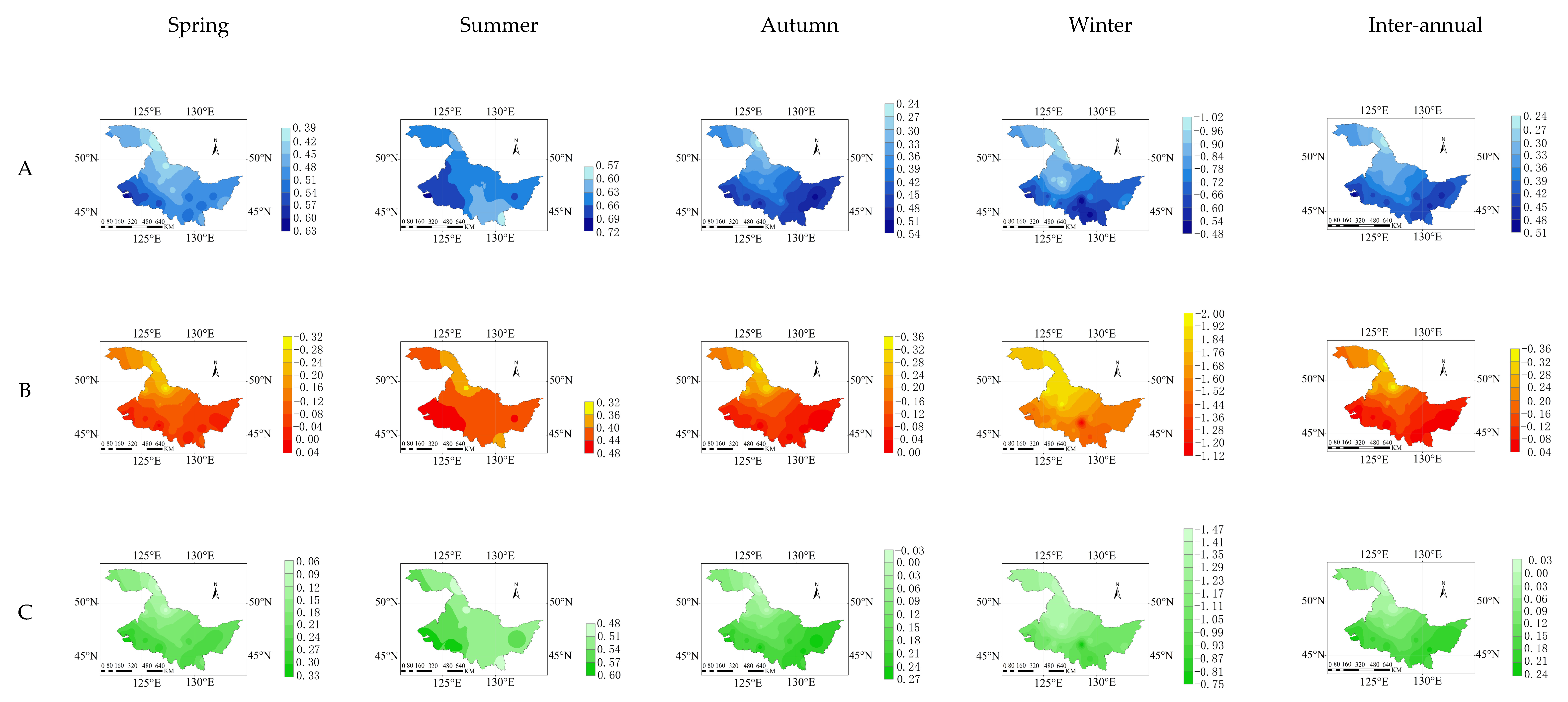
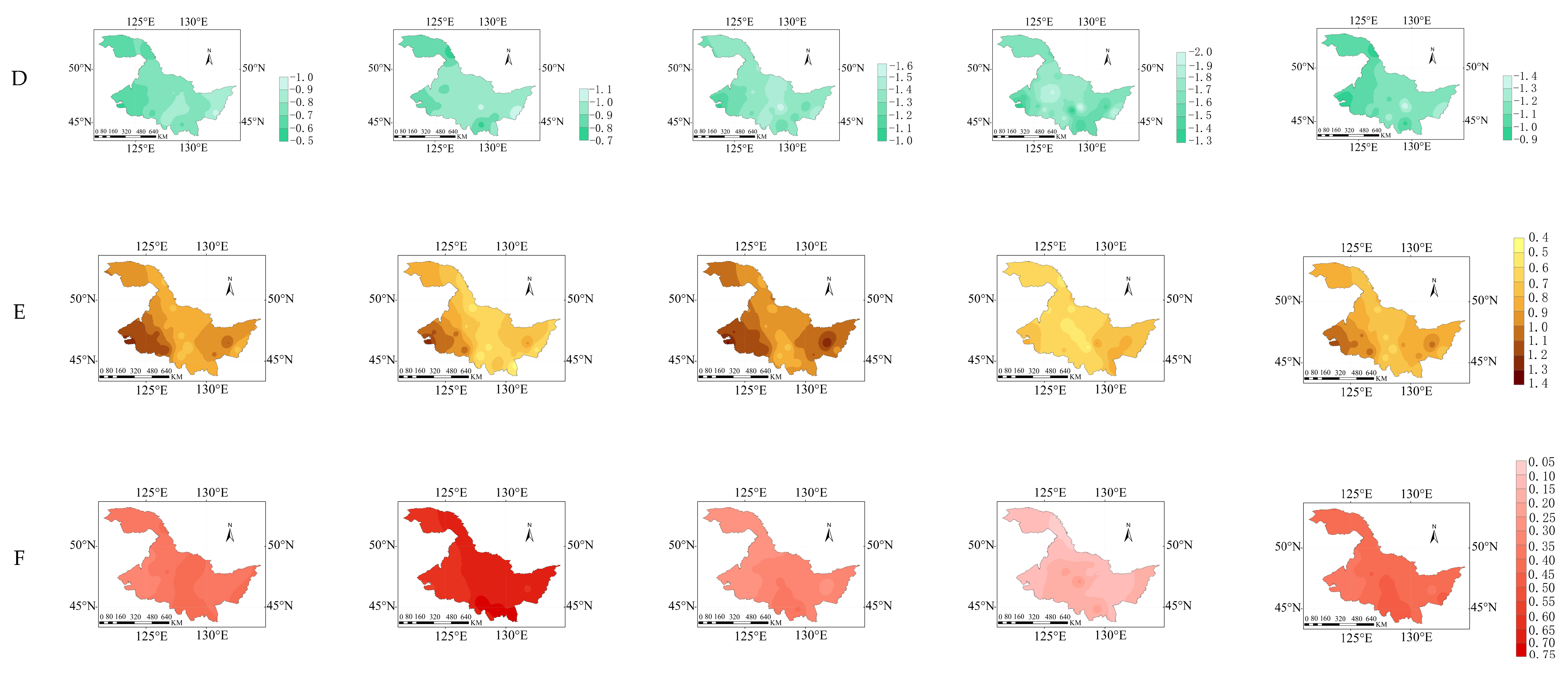
3.1. Spatial Distribution of the Mean Values of Meteorological Factors

Spatial distribution of average T_max, T_min, T_mean, RH, U, Rn from 1960 to 2019 is shown in Figure 2. On the inter-annual scale, the T_max, T_min and T_mean showed an increasing trend from north to south, their inter-annual ranges were 5.5~11.5 °C, 0.5~7.0 °C and 1.0~5.5 °C, respectively. A higher RH was mainly distributed in the central region, while the RH in east and west region was relatively lower. A higher U was mainly distributed in the east and west regions. Spatially, Rn increased from north to south.

On the seasonal scale, the T_max, T_min and T_mean also showed an increasing trend from north to south. The RH was higher in summer and lower in spring. However, the U was higher in spring and lower in summer, which were 3.71 m/s and 2.67 m/s, respectively. The Rn is larger in summer and smaller in winter; the ranges were 11.5~12.8 MJ/m² and 0.30~1.90 MJ/m², respectively.

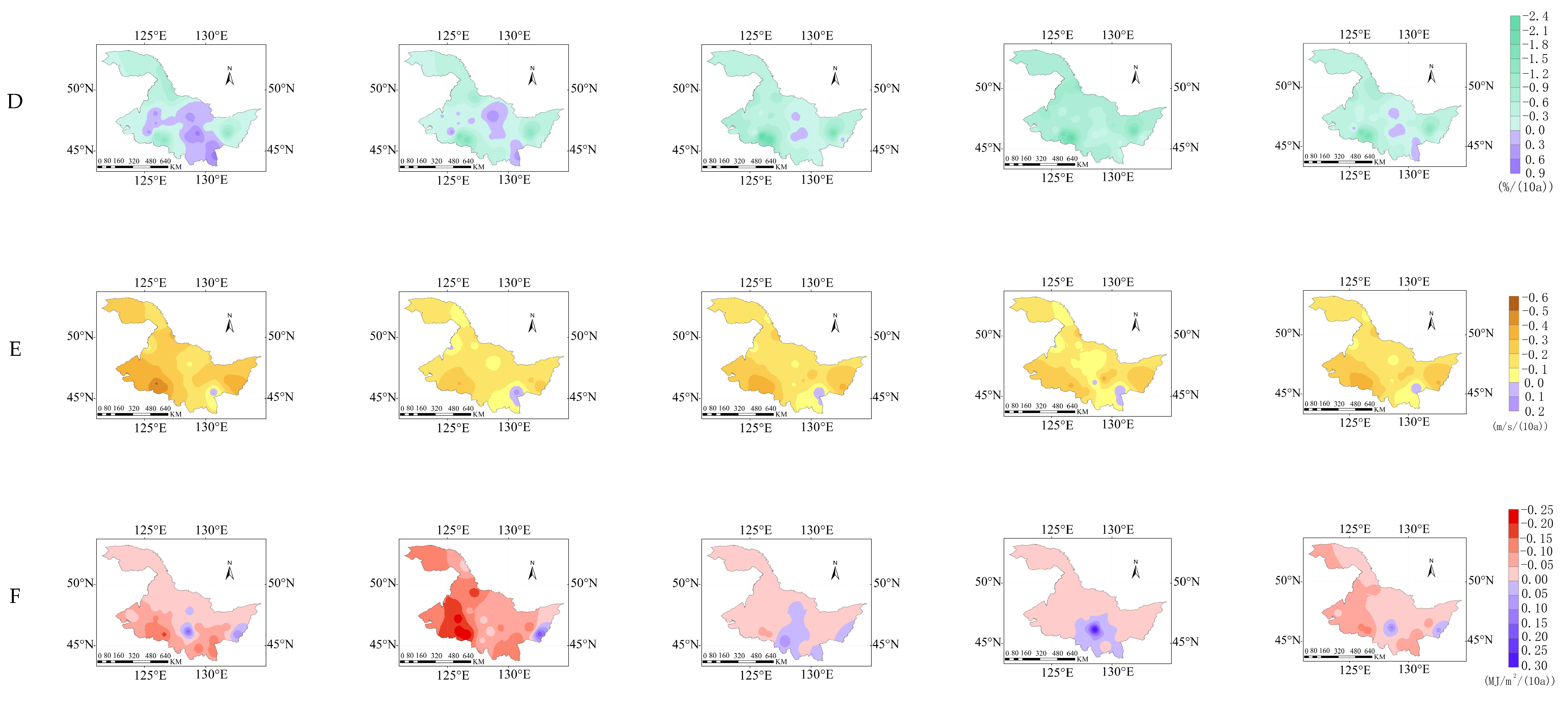
3.2. Temporal and Spatial Variation of the Climate Tendency Rate of Meteorological Factors

At time series on inter-annual and seasonal scales, the T_max, T_min, T_mean showed a significant upward trend (p < 0.05) for T_max in winter (

Table 1. Seasonal and inter-annual climate tendency rate of meteorological factors in Heilongjiang Province.

Climatic Factors	Spring	Summer	Autumn	Winter	Inter-Annual
Tmax (°C/(10a))	0.25 *	0.16 *	0.19 *	0.28	0.22 *
Tmin (°C/(10a))	0.57 *	0.39 *	0.43 *	0.65 *	0.49 *
Tmean (°C/(10a))	0.41 *	0.26 *	0.31 *	0.47 *	0.36 *
RH (%/(10a))	−0.13	−0.28	−0.51 *	−0.78 *	−0.42 *
U (m/s/(10a))	−0.24 *	−0.14 *	−0.18	−0.15 *	−0.18 *
Rn (MJ/m2/(10a))	−0.05 *	−0.10 *	−0.01	−0.01	−0.04 *

Note: * indicates a significant level of 0.05.

). Whereas, the RH, U and Rn showed a significant downward trend (p < 0.05), except for RH in spring and summer, U in autumn and Rn in autumn and winter. The inter-annual climate tendency rate for the T_max, T_min, T_mean, RH, U and Rn was 0.22 °C/10a, 0.49 °C/10a, 0.36 °C/10a, −0.42 (%/10a), −0.18 (m/s/10a), and −0.04 (MJ/m²/10a), respectively.

In terms of spatial distribution on inter-annual scales, the T_max, T_min, and T_mean showed an increasing trend, higher climate tendency rate of them were mainly distributed in the northern region (Figure 3). The RH showed a decreasing climate tendency rate except for some central and southern regions. The U was shown a decreasing trend except Jixi, and the climate tendency rate was lower in western and higher in central region. The Rn showed a decreasing climate tendency rate except for Hulin and Tonghe. On seasonal scales, The T_max, T_min, and T_mean showed an increasing trend except for T_max in Suifenhe and T_mean in Hulin in summer. The climate tendency rate of T_max, T_min, T_mean were greatest in winter compared with the other 3 seasons (Figure 3). The RH showed a decreasing climate tendency rate except in the central regions in spring, summer, and autumn. The climate tendency rate of U was lower in the western and eastern regions, and the climate tendency rate of Rn showed a decreasing trend except for some central and eastern regions.

3.3. Temporal and Spatial Variation of ET₀

ET₀ was the highest in summer and lowest in winter, with daily averages of 4.11 mm and 0.35 mm, respectively (Figure 4). ET₀ showed decreasing trends in seasons and inter-annual; the higher ET₀ values were mainly distributed in the southwest region. The average climate tendency rate of ET₀ in spring, summer, autumn, winter and inter-annual was −6.33 mm/(10a), −2.72 mm/(10a), −2.58 mm/(10a), −0.65 mm/(10a), and −8.69 mm/(10a), respectively (Figure 4). In the western region, the seasonal lower ET₀ climate tendency rate, especially in spring and summer, led to a more rapid decrease trend of inter-annual ET₀.

The inter-annual ET₀ in Heilongjiang Province showed a significant increasing trend from 1977 to 1983 (Z > 1.96), while it showed a significant decreasing trend in 2017–2019 (Z < −1.96). The mutation point of ET₀ appeared in 2011, and the changing trend of ET₀ changed from increase to decrease (Figure 5e). On a seasonal scale, the mutation years range from 2006 to 2015 (Figure 5a–d).

3.4. Sensitivity of ET₀ to Meteorological Factors

The sensitivity coefficients of ET₀ to U, Rn, RH, T_max, T_min and T_mean are shown in

Table 2. Sensitivity coefficients of seasonal and inter-annual ET₀ change to climate factors.

Season	U	Rn	RH	Tmax	Tmin	Tmean
Spring	1.35	0.36	−0.12	0.44	−0.10	0.25
Summer	0.40	0.65	−0.91	0.69	0.41	0.55
Autumn	1.40	0.28	−1.34	0.39	−0.14	0.15
Winter	0.53	0.10	−1.67	−1.64	−1.76	−1.32
Inter-annual	1.22	0.40	−1.15	0.42	−0.14	0.14

. On the inter-annual scale, in the case that other climatic factors remain unchanged, when the U, Rn, T_max, T_mean, RH and T_min increase by 10%, ET₀ will increase by 12.2%, 4.0%, 4.2%, 1.4% or decrease by 11.5% and 1.4%, respectively. The sensitivity order of ET₀ change to each climatic factor was U > RH > T_max > Rn > T_min = T_mean.

On the seasonal scale (Table 2), the changes of ET₀ in spring, summer and autumn were all negatively sensitive to RH, positively sensitive to U, Rn, T_max, and T_mean, while the changes of ET₀ to RH, T_max, T_min and T_mean were negatively sensitive in winter. ET₀ was most sensitive to U in spring and autumn, and most sensitive to RH and T_min in summer and winter, with sensitivity coefficients of 1.35, 1.40, −0.91 and −1.76, respectively.

Figure 6 shows the spatial distribution of sensitivity coefficients of ET₀. On the inter-annual scale, The sensitivity coefficients of ET₀ to T_max, T_min and T_mean gradually increased from north to south. The sensitivity coefficients of ET₀ to RH decreased from west to east. A higher sensitivity coefficient to U was mainly distributed in the eastern and western regions, while the sensitivity coefficient to Rn was mainly distributed in the central region.

On the seasonal scales, the sensitivity of ET₀ to T_max, T_min, T_mean was higher in the western region in spring and summer, and higher in the southeast and south in autumn and winter. ET₀ showed lower sensitivity to RH in the central region throughout the 4 seasons, the sensitivity coefficient of ET₀ to U was higher in spring and autumn, while the sensitivity coefficient of ET₀ to Rn was higher in summer.

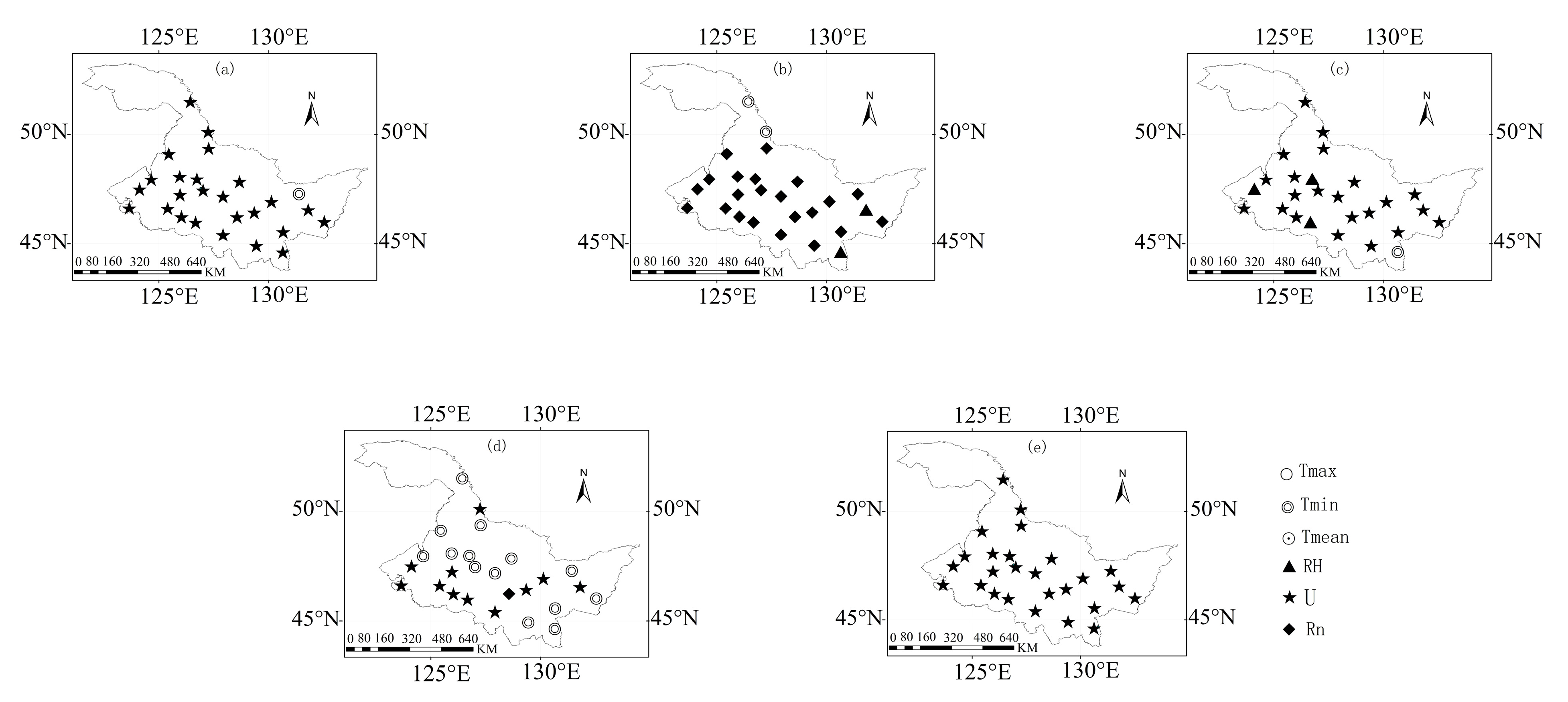
3.5. Dominant Climatic Factors for ET₀ Change

On the inter-annual scale, U was the dominant climatic factor for the change of ET₀, followed by T_max, T_mean, RH, Rn and T_min, with contribution rates of 6.15%, 5.03%, 4.34%, −1.82%, and −1.41%, respectively (

Table 3. Contribution of seasonal and inter-annual climate factors to ET₀ changes from 1960 to 2019.

Time Scales	Contribution Rates/%						Total Contribution/%	Dominant Factor
	U	Rn	RH	Tmax	Tmin	Tmean
Spring	−9.79	−1.56	0.18	6.04	−5.82	3.14	−7.81	U
Summer	−3.63	−4.37	2.02	2.57	2.1	2.09	0.78	Rn
Autumn	−13.14	−0.3	7.33	4.7	−4.5	3.78	−2.13	U
Winter	−10.86	−0.3	3.09	−10.1	−11.46	−9.33	−38.96	Tmin
Inter-annual	−8.96	−2.82	3.34	5.15	−1.41	4.03	−0.67	U

). The positive contribution rates of RH, T_max and T_mean to ET₀ have not been able to offset the negative contribution rates of U, Rn and T_min; therefore, the ET₀ showed a decreasing trend from 1960 to 2019.

On the seasonal scale, U was the dominant factor for the decrease of ET₀ in spring and autumn, followed by T_max and RH; the largest contribution rates to the change of ET₀ were −9.79% and −13.14%, respectively. In summer, Rn was the dominant factor for ET₀ change, the contribution rates of T_max, T_min, and T_mean to ET₀ were less different, which were 2.57%, 2.1% and 2.09%,respectively, while in winter, Rn contributes the least to ET₀, and T_min became the dominant factor.

The spatial distribution of dominant meteorological factors is shown in Figure 7. In spring, the dominant factor for ET₀ was U in the study area except for Fujin (Figure 7a), In summer, Rn was the dominant factor in most regions of the study area, T_min and RH were the dominant factors in the partial northern and eastern regions. In autumn, U was the dominant factor for 85% of the total 26 sites (Figure 7c); in winter, T_min was the dominant factor in the northern and eastern regions, while U was the dominant factor in the western region. On the inter-annual scale, the dominant factor of all 26 sites was U (Figure 7e).

4. Discussion

Under the general warming of the global climate, ET₀ was on the rise in most areas, such as the annual ET₀ for India, which, as a whole, has increased in the latter half of the 20th century [31]; Awash River basin, Ethiopia [32], and South Korea over the recent 100 years [33], which is consistent with the generally accepted trend that ET₀ increases with temperature. However, the phenomenon of the “evaporation paradox” appeared in many areas around the world [34], that is, with the continuous increase of temperature, the ET₀ showed a decreasing trend, such as the Canadian prairie region, the northern region of South America, Thailand, New Zealand [9,35,36,37], and the northwest of India [38], the Lijiang watershed [39], as well as Alor Setar, Malaysia [40]. In this study, ET₀ in Heilongjiang Province from 1960 to 2019 showed a decrease trend inter-annually and seasonally with the increasing temperature, proving that the “evaporation paradox” phenomenon also existed in our study area, which was consistent with the conclusion of Li et al. [41]. At present, there is still no clear conclusion about the mechanism of the “evaporation paradox”; the existing related research studies are mostly qualitative analysis, and the reasons need to be further explored.

In China, the sensitivity coefficient and contribution rate of ET₀ to meteorological factors varied in different climatic regions. Even in the same climatic region, the sensitivity coefficient and contribution rate of ET₀ were different spatially. For example, in the subtropical monsoon climate zone, ET₀ in the Yangtze River basin [42], Sichuan basin [43], and Yunnan-Guizhou plateau [44] were most sensitive to the T_max, RH, and sunshine hours, respectively. In the temperate continental climate zone, ET₀ in the middle and upper reaches of the Yellow River [45] and the Ebinur Lake basin in Xinjiang [46] were most sensitive to the actual water vapor pressure and U, respectively, with the highest contribution rate of U for both regions. In the plateau mountainous climate region, the meteorological factor with the largest sensitivity coefficient in the Qinghai Tibet Plateau was the actual water vapor pressure, and the sunshine hours had the largest contribution rate to ET₀ [47]. Our study area is located in the temperate monsoon climate zone, where ET₀ was the most sensitive to U and had the largest contribution rate to ET₀. However, in the Loess Plateau basin, which is also located in the same climate zone, ET₀ was most sensitive to actual water vapor pressure and T_mean had the highest contribution rate [48]. In the North China Plain of the temperate monsoon climate zone, sunshine hours had the largest contribution rate to ET₀ [21]. In summary, the plateau area has strong solar radiation, long sunshine time, and low temperature, which may cause the ET₀ to be most affected by the sunshine hours; most of the basin areas have a dry climate, less rainfall, and lack of water resources, causing vegetation to be more sensitive to the water condition; therefore, RH might have a larger sensitivity coefficient to ET₀. Heilongjiang Province is located in plain and mountainous areas, and affected by southeast monsoon in summer and controlled by northwest monsoon in winter [49]. This might be the reason why U contributed the most to ET₀ change.

In this study, ET₀ in Heilongjiang Province showed a decrease trend on the inter-annual scale from 1960 to 2019, with U as the dominant factor, which was consistent with the trend of ET₀ in Jilin Province analyzed by Liu et al. [50] and in Liaoning Province analyzed by Cao et al. [51]. This was probably because the above three provinces are geographically contiguous and have a similar type of climate characteristics. A research established by Xu et al. in 2003 predicted that the temperature in Heilongjiang Province would increase significantly by 2030 and 2050 with a higher increase in winter and a lower increase in summer by the CCCma (Canadian Center for Climate Modelling and analysis), CCSR (Center for Climate System Research), CSIRO (Commonwealth Scientific and Industrial Research Organization), GFDL (Geophysical Fluid Dynamics Laboratory) and Hadley climate models [52]. Zhang et al. [53] pointed out that the climate of Heilongjiang Province would tend to be warm and humid in the next 41 years by the Hadley model. Wang et al. [54] believed that ET₀ was not only affected by various meteorological factors, but interactions between meteorological factors would also interfere with ET₀ changes. Moreover, ET₀ may also be affected by human activities including aerosol emissions, air pollution [55] and rice area expansion [56]. Therefore, further exploration in these aspects will be needed for contribution analysis of ET₀ changes in Heilongjiang Province in the future, as well as in other regions of the world.

5. Conclusions

In this study, ET₀ was calculated by the Penman–Monteith formula, the sensitivity-contribution rate method was used to clarify the climatic factors affecting seasonal and inter-annual changing of ET_0., The T_max, T_min, T_mean showed an increasing trend and RH, U, Rn showed a decreasing trend from 1960 to 2019. ET₀ showed a decreasing trend with an average climate tendency rate of −8.69 mm/(10a). The annual average ET₀ change was negatively sensitive to T_min and RH, and positively sensitive to T_max, T_mean, U and Rn. U was the dominant factor for the ET₀ decrease in spring and autumn, while RH and T_min were the dominant factors in summer and winter, respectively. On the inter-annual scale, the sensitivity order of ET₀ change to each climatic factor was U > RH > T_max > Rn > T_min = T_mean. These results indicated that the dominant factors for ET₀ changes were U in Heilongjiang Province. Moreover, the dominant factors for ET₀ change varies under different climatic and geographical conditions; impacts of human activities on ET₀ should also be considered in future studies.

References

1. IPCC. Climate Change 2007: The Physical Science Basis; Cambridge University Press: Cambridge, UK, 2007. [Google Scholar]
2. Silva, C. Importance of modelling and its feasibility in the future climate in Sri Lanke. Symp. Water Prof. Day 2013, 18, 15–28. [Google Scholar]
3. Anabalón, A.; Sharma, A. On the divergence of potential and actual evapotranspiration trends: An assessment across alternate global datasets. Earth’s Future 2017, 9, 905–917. [Google Scholar] [CrossRef]
4. Ding, Y.H. Introduction to Climate Change Science in China; China Meteorological Press: Beijing, China, 2008; Volume 128. [Google Scholar]
5. Abedi-Koupai, J.; Dorafshan, M.M.; Javadi, A. Estimating potential reference evapotranspiration using time series models (case study: Synoptic station of Tabriz in northwesternIran). Appl. Water Sci. 2022, 12, 212. [Google Scholar] [CrossRef]
6. Li, Y.L.; Cui, J.Y.; Zhang, T.H. A comparative study on the calculation methods of reference crop evapotranspiration. China Desert 2002, 04, 65–69. [Google Scholar]
7. Pereira, L.S.; Allen, R.G.; Smith, M. Crop evapotranspiration estimation with FAO56: Past and future. Agric. Water Manag. 2015, 147, 4–20. [Google Scholar] [CrossRef]
8. Jung, M.; Reichstein, M.; Ciais, P.; Seneviratne, S.I.; Goulden, M.L.; Bonan, G.; Cescatti, A.; Chen, J.Q.; De, J. Recent decline in the global land evapotranspiration trend due to limited moisture supply. Nature 2010, 467, 951–954. [Google Scholar] [CrossRef] [PubMed] [Green Version]
9. Roderick, M.L.; Farquhar, G.D. Changes in New Zealand pan evaporation since the 1970s. Int. J. Climatol. 2005, 25, 2031–2039. [Google Scholar] [CrossRef]
10. Onyutha, C. Statistical analyses of potential evapotranspiration changes over the period 1930–2012 in the Nile River riparian countries. Agric. For. Meteorol. 2016, 226–227, 80–95. [Google Scholar] [CrossRef]
11. Dadaser-Celik, F.; Cengiz, E.; Guzel, O. Trends in reference evapotranspiration in Turkey: 1975–2006. Int. J. Climatol. 2016, 36, 1733–1743. [Google Scholar] [CrossRef] [Green Version]
12. Wu, X.; Wang, P.J.; Huo, Z.G.; Bai, Y.M. Spatio-temporal distribution characteristics of potential evapotranspiration and impact factors in China from 1961 to 2015. Resour. Sci. 2017, 39, 964–977. [Google Scholar]
13. Bandyopadhyay, A.; Bhadra, A.; Raghuwanshi, N.S.; Singh, R. Temporal trends in estimates of reference evapotranspiration over India. J. Hydrol. Eng. 2014, 14, 508–515. [Google Scholar] [CrossRef]
14. Roderick, M.L.; Farquhar, G.D. Changes in Australian pan evaporation from 1970 to 2002. Int. J. Climatol. 2004, 24, 1077–1090. [Google Scholar] [CrossRef]
15. Tabari, H.; Talaee, P.H. Sensitivity of evapotranspiration to climatic change in different climates. Glob. Planet. Chang. 2014, 115, 16–23. [Google Scholar] [CrossRef]
16. Guo, D.L.; Westra, S.; Holger, R.M. Sensitivity of potential evapotranspiration to changes in climate variables for different Australian climatic zones. Hydro. Earth Syst. Sci. 2017, 21, 2107–2126. [Google Scholar] [CrossRef] [Green Version]
17. Zhang, Z.G.; Zheng, M.J.; Cai, M.T.; Yin, J.Y.; Li, H.H.; Wang, Y.W. Spatio-temporal evolution and genesis analysis of reference crop evapotr-anspiration in Henan Province from 1960 to 2019. Water Sav. Irrig. 2021, 3, 44–50. (In Chinese) [Google Scholar]
18. Wu, W.Y.; Kong, Q.Q.; Wang, X.D.; Ma, X.Q.; He, B.F.; Zhang, H.Q. Sensitivity analysis of reference crop evapotranspiration in Anhui Province in the past 40 years. J. Ecol. Environ. 2013, 22, 1160–1166. [Google Scholar]
19. Zhao, L.; Liang, C. Study on the causes of changes in potential evapotranspiration in Sichuan Province in the past 50 years. Soil Water Conserv. Res. 2014, 21, 26–30. (In Chinese) [Google Scholar]
20. Wang, X.D.; Ma, X.Q.; Xu, Y.; Lui, R.N.; Cao, W.; Zhu, H. The variation characteristics of reference crop evapotranspiration and the contribution of main meteorological factors in the Huaihe River Basin. China Agric. Meteorol. 2013, 34, 661–667. (In Chinese) [Google Scholar]
21. Wang, P.T.; Yan, J.P.; Jiang, C.; Liu, X.F. Spatial-temporal variation of reference crop evapotranspiration and its influencing factors in North China Plain. Acta Ecol. Sin. 2014, 34, 5589–5599. [Google Scholar]
22. Zhou, B.R.; Li, F.X.; Xiao, H.B.; Hu, A.J.; Yan, L.D. Temporal and spatial differentiation characteristics of potential evapotranspiration and climate attribution in the source region of the Three Rivers. J. Nat. Resour. 2014, 29, 2068–2077. [Google Scholar]
23. Wang, Q.J.; Lv, J.J.; Li, X.F.; Wang, P.; Ma, G.Z. Distribution characteristics of agricultural meteorological disasters in Heilongjiang Province and their impact on agricultural production. Heilongjiang Water Conserv. Sci. Technol. 2016, 44, 57–61. (In Chinese) [Google Scholar]
24. Zhang, P. Analysis on the Causes of Agricultural Natural Disasters in Heilongjiang Province. Res. Agric. Mech. 2011, 33, 249–252. [Google Scholar]
25. Nie, T.Z.; Tang, Y.; Jiao, Y.; Li, N.; Wang, T.Y.; Du, C.; Zhang, Z.X.; Chen, P.; Li, T.C.; Sun, Z.Y.; et al. Effects of Irrigation Schedules on Maize Yield and Water Use Efficiency under Future Climate Scenarios in Heilongjiang Province Based on the AquaCrop Model. Agronomy 2022, 12, 810. [Google Scholar] [CrossRef]
26. Jiang, Y.; Du, C.; Sun, H.N.; Zhong, Y. Spatio-temporal variation characteristics and sensitivity analysis of potential evapotranspiration during crop growing season in Heilongjiang Province under climate change. Hydropower Energy Sci. 2018, 36, 6–9. (In Chinese) [Google Scholar]
27. Su, J.W.; Zhang, X.L.; Shen, B. Spatio-temporal variation characteristics and influencing factors of potential evapotranspiration in Heilongjiang. Heilongjiang Water Conserv. Sci. Technol. 2021, 49, 1–8. (In Chinese) [Google Scholar]
28. Tu, A.G.; Li, Y.; Nie, X.F.; Mo, M.H. Changes of reference crop evapotranspiration in Poyang Lake Basin and its attribution analysis. Ecol. Environ. Sci. 2017, 26, 211–218. [Google Scholar]
29. Xing, L.T.; Huang, L.X.; Chi, G.Y.; Yang, L.Z.; Li, C.S.; Hou, X.Y. A Dynamic Study of a Karst Spring Based on Wavelet Analysis and the Mann-Kendall Trend Test. Water 2018, 10, 698. [Google Scholar] [CrossRef] [Green Version]
30. Xing, H.H.; Chen, H.D.; Lin, H.Y. Sensitivity analysis of hierarchical hybrid fuzzy-neural network based on input perturbation. Software 2013, 34, 52–55. [Google Scholar]
31. Sarma, A.; Bhaskar, V.V.; Sastry, C.M. Potential Evapotranspiration over India—An estimate of Green Water flow. Mausam 2014, 65, 365–378. [Google Scholar] [CrossRef]
32. Yadeta, D.; Kebede, A.; Tessema, N. Potential evapotranspiration models evaluation, modelling, and projection under climate scenarios, Kesem sub-basin, Awash River basin, Ethiopia. Model. Earth Syst. Environ. 2020, 6, 2165–2176. [Google Scholar] [CrossRef]
33. Jeon, M.G.; Nam, W.H.; Mun, Y.S.; Yoon, D.H.; Yang, M.H.; Lee, H.J.; Shin, J.H.; Hong, E.M.; Zhang, X. Climate change impacts on reference evapotranspiration in South Korea over the recent 100 years. Theor. Appl. Climatol. 2022, 150, 309–326. [Google Scholar] [CrossRef]
34. Roderick, M.L.; Farquhar, G.D. The cause of decreased pan evaporation over the past 50 years. Science 2002, 298, 1410–1411. [Google Scholar] [CrossRef] [PubMed]
35. Burn, D.H.; Hesch, N.M. Trends in evaporation for the Canadian Prairies. J. Hydrol. 2007, 336, 61–73. [Google Scholar] [CrossRef]
36. Quintana-Gomez, R.A. Changes in evaporation patterns detected in northernmost South America: Homogeneity testing. In Proceedings of the 7th International Meeting on Statistical Climatology, Whisler, BC, Canada, 25–29 May 1998. [Google Scholar]
37. Tebakari, T.C.; Yoshitani, J.C.; Suvanpimol, C.C. Time-space trend analysis in pan evaporation over Kingdom of Thailand. J. Hydrol. Eng. 2005, 10, 205–215. [Google Scholar] [CrossRef]
38. Das, P.K.; Midya, S.K.; Das, D.K.; Rao, G.S.; Raj, U. Characterizing Indian meteorological moisture anomaly condition using long-term (1901–2013) gridded data: A multivariate moisture anomaly index approach. Int. J. Climatol. 2018, 38, E144–E159. [Google Scholar] [CrossRef]
39. Jiao, L.; Wang, D.M. Climate Change, the Evaporation Paradox, and Their Effects on Streamflow in Lijiang Watershed. Pol. J. Environ. Stud. 2018, 27, 2585–2591. [Google Scholar] [CrossRef]
40. Ahmad, A.A.; Yusof, F.; Mispan, M.R.; Kamaruddin, H. Rainfall, evapotranspiration and rainfall deficit trend in Alor Setar, Malaysia. Malays. J. Fundam. Appl. Sci. 2017, 13, 400–404. [Google Scholar] [CrossRef]
41. Li, X.F.; Jiang, L.X.; Li, X.F.; Zhao, F.; Zhu, H.X.; Wang, P.; Gong, L.J.; Zhao, H.Y. Evolution characteristics of evaporation and its relationship with climatic factors in Heilongjiang Province from 1961 to 2017. Meteorology 2021, 47, 755–766. (In Chinese) [Google Scholar]
42. Liu, C.M.; Zhang, D.; Liu, X.M.; Zhao, C.S. Spatial and temporal change in the potential evapotranspiration sensitivity to meteorological factors in China (1960–2007). J. Geogr. Sci. 2012, 22, 3–14. (In Chinese) [Google Scholar] [CrossRef]
43. Chen, D.D.; Wang, X.D.; Wang, S.; Su, X.W. Variation of potential evapotranspiration and its climatic influencing factors in Sichuan Province. Chin. J. Agrometeorol. 2017, 38, 548–557. (In Chinese) [Google Scholar]
44. Yu, F.; Gu, X.P.; Xiong, H. Spatio-temporal variation characteristics of potential evapotranspiration in Guizhou and sensitivity to meteorological factors. Agric. Sci. Technol. 2015, 16, 2845–2848. (In Chinese) [Google Scholar]
45. Wang, Y.J.; Li, J.; Lin, Z.H.; Tong, X.J.; Xing, X.M. Estimation of the potential evapotranspiration effects of climate change on the middle and upper reaches of the Yellow River. Chin. J. Soil Water Conserv. 2013, 11, 48–56. (In Chinese) [Google Scholar]
46. Xu, J.J.; Jin, X.Y.; Qiang, H.F.; Dai, H.; Liang, C. Characteristics and causes of potential evapotranspiration change in The Ebi Lake Basin in Xinjiang. J. Irrig. Drain. 2018, 37, 89–94. [Google Scholar]
47. Shi, Y. Climate Change on the Tibetan Plateau and Its Impact on Potential Evapotran-Spiration; Beijing Forestry University: Beijing, China, 2019. [Google Scholar]
48. Ning, T.T. Spatial-Temporal Variation of Evapotranspiration in the Loess Plateau under Budyko Framework and Its Attribution Analysis; Research Center for Soil and Water Conservation and Eco-Environment of the Ministry of Education; Chinese Academy of Sciences: Beijing, China, 2017. (In Chinese) [Google Scholar]
49. Chen, P.; Xu, J.; Zhang, Z.; Wang, K.; Li, T.; Wei, Q.; Li, Y. Carbon pathways in aggregates and density fractions in Mollisols under water and straw management: Evidence from 13C natural abundance. Soil. Biol. Biochem. 2022, 169, 108684. [Google Scholar] [CrossRef]
50. Liu, Y.X.; Ren, J.Q.; Wang, D.N.; Mu, J.; Cui, J.L.; Chen, C.S.; Chen, X.; Guo, C.M. Spatio-temporal distribution and genesis analysis of reference crop evapotranspiration in Jilin Province. J. Ecol. Environ. 2019, 28, 2208–2215. [Google Scholar]
51. Cao, Y.Q.; Qi, J.W.; Wang, F.; Li, L.H.; Lu, J. Evolution law and attribution analysis of potential evapotranspiration in Liaoning Province. Acta Ecol. Sin. 2020, 40, 3519–3525. [Google Scholar]
52. Xu, N.P.; Pan, H.S.; Xu, Y.; Zhang, G.H. Climate change prediction of Heilongjiang Province in the next 30 and 50 years. J. Nat. Disasters 2004, 1, 146–150. [Google Scholar]
53. Zhang, J.T.; Feng, L.P.; Pan, Z.H. Climate change trend and mutation analysis in Heilongjiang Province in the next 41 years. Meteorol. Environ. 2014, 37, 60–66. [Google Scholar]
54. Wang, Q.; Zhang, M.J.; Pan, S.K.; Ma, X.N.; Li, F.; Liu, W.L. Spatial-temporal variation characteristics of potential evapotranspiration in the Yangtze River Basin. Chin. J. Ecol. 2013, 32, 1292–1302. (In Chinese) [Google Scholar]
55. Ning, T.; Li, Z.; Liu, W.; Han, X. Evolution of potential evapotranspiration in the northern Loess Plateau of China: Recent trends and climatic drivers. Int. J. Climatol. 2016, 36, 4019–4028. [Google Scholar] [CrossRef]
56. Hu, X.; Chen, M.; Liu, D.; Li, D.; Jin, L.; Liu, S.; Cui, Y.; Dong, B.; Khan, S.; Luo, Y. Reference evapotranspiration change in Heilongjiang Province, China from 1951 to 2018: The role of climate change and rice area expansion. Agric. Water Manag. 2021, 253, 106912. [Google Scholar] [CrossRef]
Figure 1. Map of the study area and distribution of meteorological stations in Heilongjiang Province.
Agriculture 12 02017 g001
Figure 2. Spatial distribution of average (Row A) Tmax, (Row B) Tmin, (Row C) Tmean, (Row D) RH, (Row E) U, (Row F) Rn from 1960 to 2019.
Agriculture 12 02017 g002aAgriculture 12 02017 g002b
Figure 3. Climatic tendency rate of (Row A) Tmax, (Row B) Tmin, (Row C) Tmean, (Row D) RH, (Row E) U, (Row F) Rn from 1960 to 2019.
Agriculture 12 02017 g003aAgriculture 12 02017 g003b
Figure 4. (Row A) spatial distribution and (Row B) climate tendency of ET0 from 1960 to 2019.
Agriculture 12 02017 g004
Figure 5. Mann–Kendall (MK) analysis of ET0 in (a) spring, (b) summer, (c) autumn, (d) winter and (e) inter-annually from 1960 to 2019.
Agriculture 12 02017 g005
Figure 6. Spatial distribution of sensitivity coefficients of ET0 to (Row A) Tmax, (Row B) Tmin, (Row C) Tmean, (Row D) RH, (Row E) U, (Row F) Rn from 1960 to 2019.
Agriculture 12 02017 g006aAgriculture 12 02017 g006b
Figure 7. Spatial distribution of dominant climatic factors in (a) spring, (b) summer, (c) autumn, (d) winter and (e) inter-annually in the study area from 1960 to 2019.
Agriculture 12 02017 g007