
Towards the Modeling and Prediction of the Yield of Oilseed Crops: A Multi-Machine Learning Approach


Abstract
1. Introduction

| Application | Performance Prediction | Model | RMSE (R2) * | Ref. |
|---|---|---|---|---|
| Seed and Crop Yield | Prediction of oilseed rape yield with alternative planting styles and varied nitrogen fertilizer applications. | SVR ANN PLSR | - | [54] |
| Estimation of soybean seed yield using collected multispectral images for predictions. | MLP | - | [55] | |
| Incorporation of multi-qualitative and quantitative features for the estimation of wheat yields. | ANN | - | [56] | |
| ML model comprised of high-dimensional phenotypic trait data to carry out in-season seed yield predictions. | RF | - (0.83) | [57] | |
| Ten agro-morphological and phenological traits (plant height, number of branches per plant, number of capsules per plant, number of days to flowering, number of days to maturity, thousand-seed weight, etc.) were used as the basis for a predictive seed yield model. | ANN MLP RBF PCA | 0.87 (0.92) | [16,58] | |
| Prediction of crop yields in mustard and potato with models using soil elemental properties, physicochemical features, pH, electrical conductivity, organic carbon, and others for training and test datasets. | ANN SVR KNN | - 4.62 (0.72) | [59,60] | |
| Prediction of corn crop yield by careful climate change factor (temperature and moisture) evaluation to compile an impact assessment of corn fields. | ANN | 1.5 | [61] | |
| ML to provide predictive estimates of the maize crop yield using topography, land use, soil data, and multiple other parameters. | - | (0.96) | [62] | |
| Yield predictions of rice paddies using climate-based factors (rainfall, morning and evening relative humidity, minimum and maximum temperature). | ANN | 31 | [63] | |
| Utilization of fertilizer volume in tandem with general atmospheric conditions to predict maize yields. | ANN MR | 30 | [64] | |
| Predictions of rice paddy yields based on environmental features (area, number of open wells, tanks, maximum temperature, etc.) as independent variables. | ANN MLR SVR RF | 0.05–0.1 (0.8) | [65] | |
| Constructing several distinct ML models to predict winter rapeseed yield at specific timepoints from six agro-morphological traits (oil and protein content, seed yield, oil and protein yield, and thousand-seed weight) as inputs. | ANN RF | - (0.944) | [66,67] | |
| Examination of micro-topographic attributes related to growth in agronomic crops based on analyses of vegetation indices, lidar derivatives, and crop type. | ANN | - | [68] | |
| Investigation of available water holding capacity of soil coupled with climate data, used to estimate the average wheat yield within a region. | ANN | - | [69] | |
| Cotton lint yield derived from a remote sensing ANN model evaluating eight phenological crop indices. | ANN | - | [70] | |
| Six ML algorithms applied to predict the cotton yield by climate and management parameters. | ANN, RF, etc. | (0.51) | [49] | |
| Predicted and optimized the corn yield by ML technique. | - | 9 | [71] | |
| Some seed and crop yields, such as maize, sorghum, and groundnut, modeled by climate data. | - | - | [72] | |
| NN-based ML applied to predict the chemical specification (fatty acid) of rubber seed oil | ANN and ANFIS | (0.69 to 0.99) | [73] | |
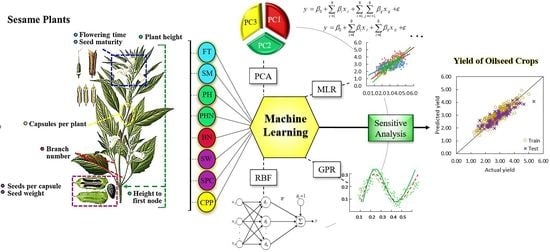
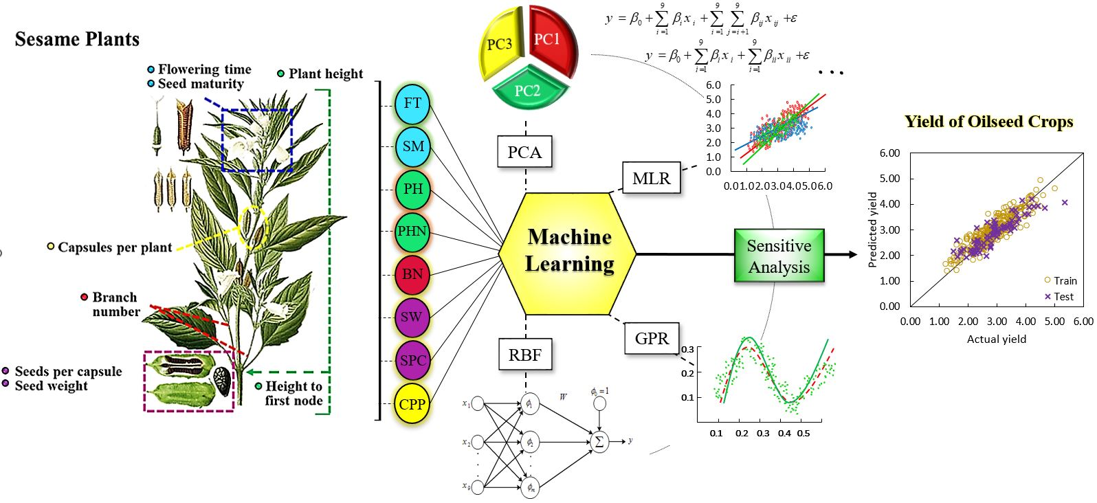
| Prediction of seed yield with ML and coupled PCA-ML models accompanied by sensitivity analysis based on agro-morphological features of sesame plants. | MLR PCA RBF GPR | 0.00–0.36 (0.88–0.99) | This work | |
| Seed classification | 14 categories of seeds and date fruits are classified by utilizing deep learning. | CNNs | (0.99) | [74,75] |
| ML applied to classify various seeds by using simple architecture and memory characteristics. | CNNs | (0.98) | [76] | |
| Nitrogen and Oil Concentration | Nitrogen prediction of oilseed rape leaves based on ten spectral features from both barley and oilseed rape. | ANN | 0.30 (0.9) | [77,78] |
| The merging of bio-physiochemical and spectral features in leaves for further in-depth studies. | GP | 2.2–5.8 | [79] | |
| Prediction of sesame oil content from eighteen agro-morphological and phonological traits using ML in efforts to prevent marginal effects. | ANN MLR PCA | 0.56 (0.86) | [80] | |
| Disease and Quality Diagnoses for use in Classification | Integration of ML models coupled with hyperspectral imaging to detect disease in pre-symptomatic tobacco plants. | LS-SVM | - | [81] |
| Conducting an oilseed disease analysis with directed surveys of ten common oilseed disease classes. | DT RF MLP | - | [82] | |
| Investigation of physicochemical properties (fatty acid and mineral profiles) and additional physical attributes of six sunflower varieties for use in classification, grading, and quality assessment studies. | SVM, RF, MLR, etc. | 0.21 (0.81) | [83] |
- Four ML models were employed to aid in predicting the sesame seed yield (SSY).
- Coupled PCA-ML models were used for in-depth predictions of SSY for the first time.
- The use of the GPR, RBF, and MLR models led to a greater accuracy of the SSY predictions.
- The primary agro-morphological features for predicting the SSY were revealed through a sensitivity analysis.

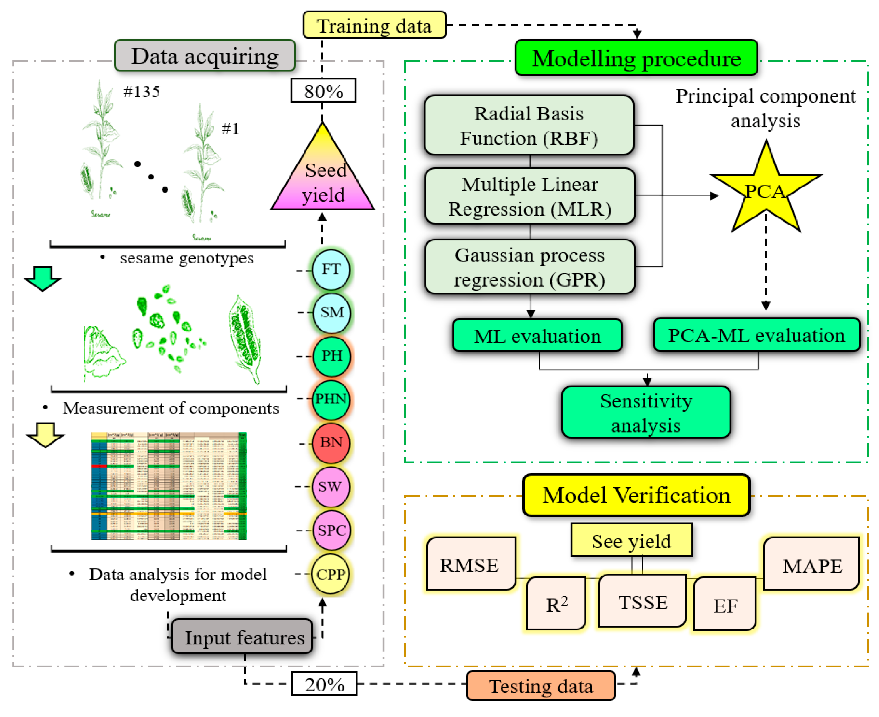
2. Material and Method
2.1. Field Experiments
2.2. Machine Learning Algorithms and Models
2.2.1. Multiple Linear Regression (MLR) Models
2.2.2. Principal Component Analysis (PCA)
2.2.3. Gaussian Process Regression (GPR) Model
2.2.4. Radial Basis Function (RBF) Neural Network
2.3. K-Fold Cross-Validation
2.4. Model Assessment Criteria
3. Results and Discussions
3.1. Primary Statistical Analysis of Datasets
3.2. Statistical Processes of PCA and MLR Algorithms
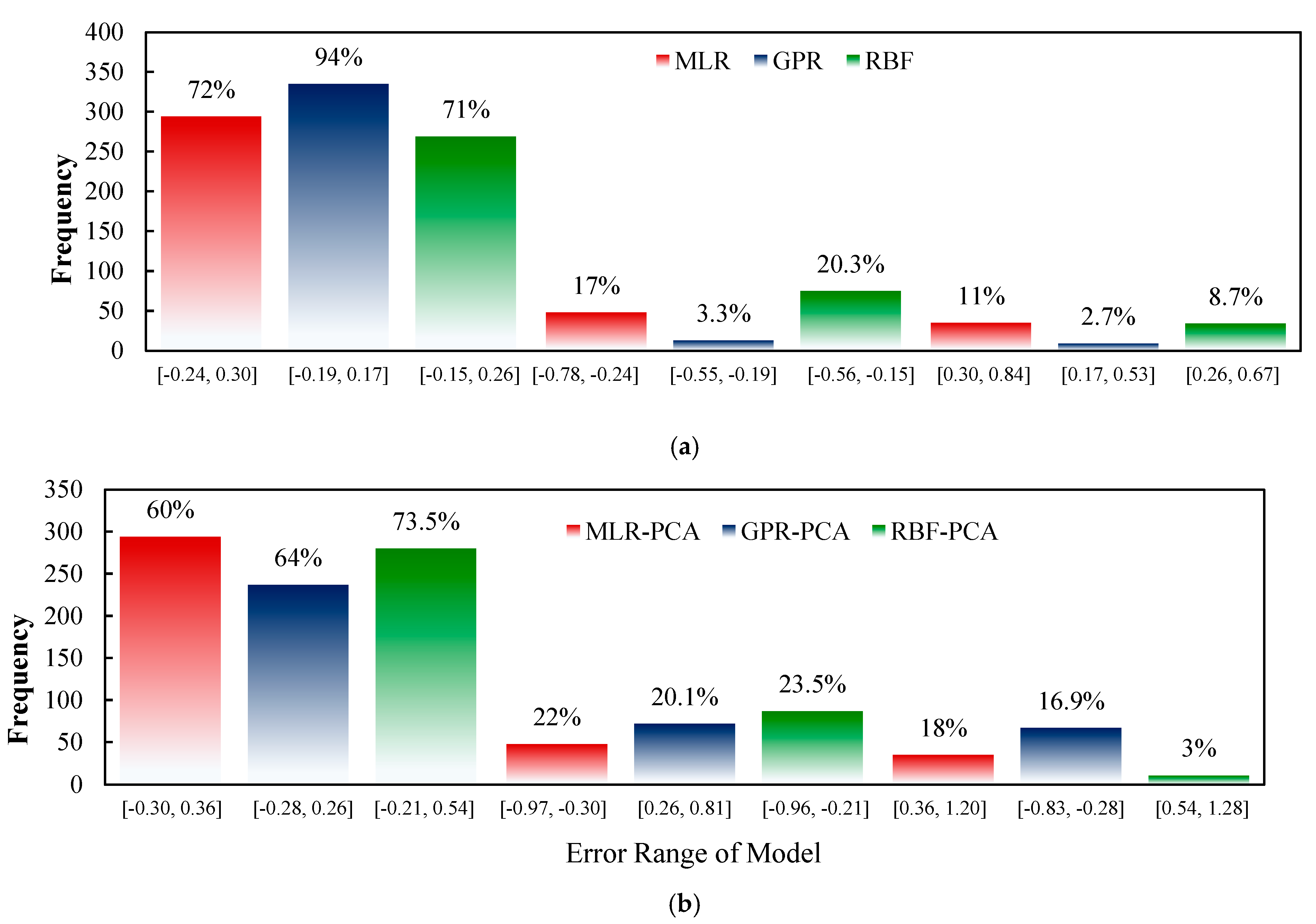
3.3. ML Models Evaluation
3.4. Prediction of Sesame-Seed-Yield-Based ML Models
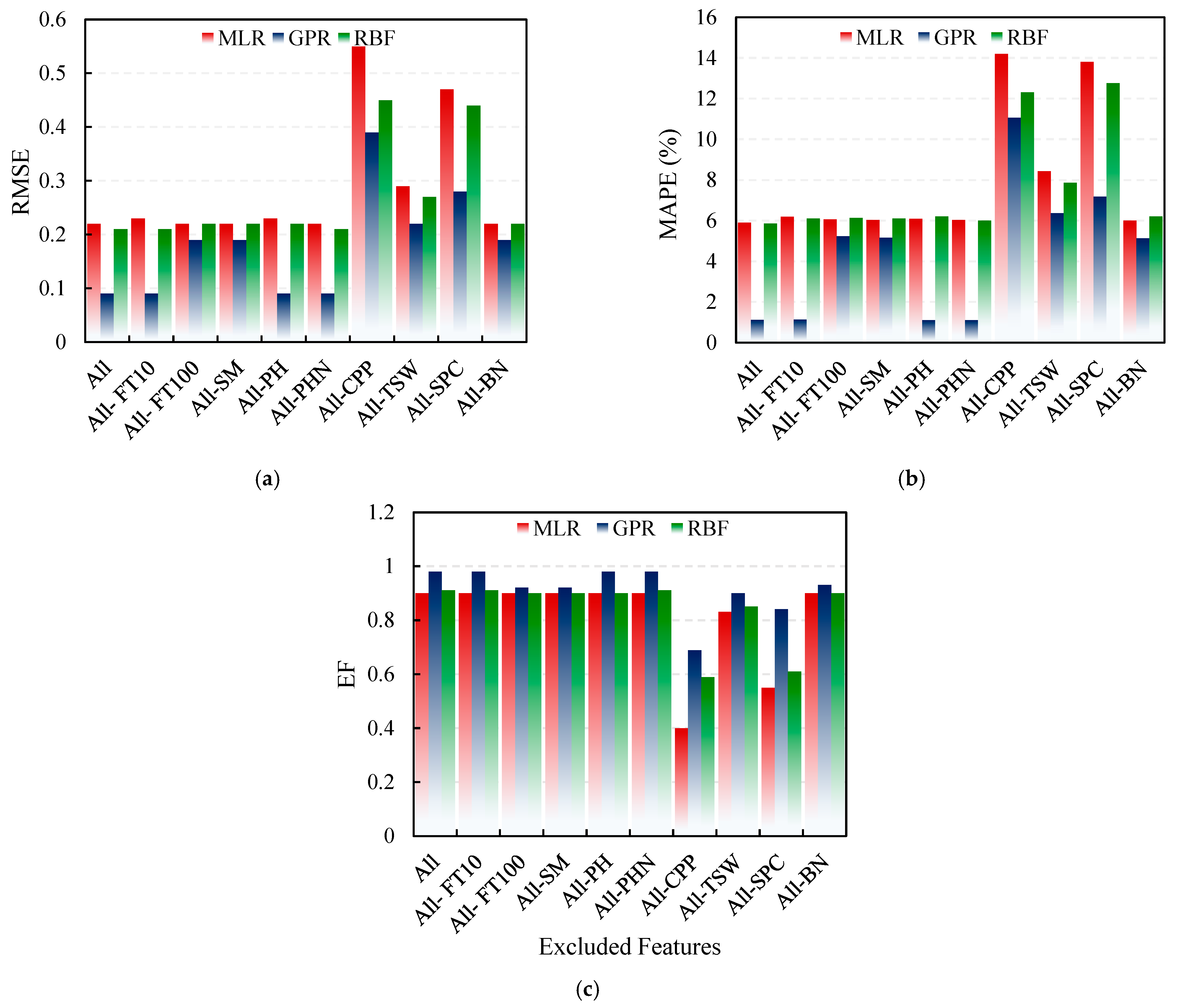
3.5. Sensitivity Analysis
4. Conclusions
Author Contributions
Funding
Institutional Review Board Statement
Informed Consent Statement
Data Availability Statement
Acknowledgments
Conflicts of Interest
References
- Bassegio, D.; Zanotto, M.D.; Santos, R.F.; Werncke, I.; Dias, P.P.; Olivo, M. Oilseed crop crambe as a source of renewable energy in Brazil. Renew. Sustain. Energy Rev. 2016, 66, 311–321. [Google Scholar] [CrossRef]
- Mousavi-Avval, S.H.; Shah, A. Techno-economic analysis of hydroprocessed renewable jet fuel production from pennycress oilseed. Renew. Sustain. Energy Rev. 2021, 149, 111340. [Google Scholar] [CrossRef]
- Ikegami, M.; Wang, Z. Does energy aid reduce CO2 emission intensities in developing countries? J. Environ. Econ. Policy 2021, 10, 343–358. [Google Scholar] [CrossRef]
- Agidew, M.G.; Dubale, A.A.; Atlabachew, M.; Abebe, W. Fatty acid composition, total phenolic contents and antioxidant activity of white and black sesame seed varieties from different localities of Ethiopia. Chem. Biol. Technol. Agric. 2021, 8, 14. [Google Scholar] [CrossRef]
- Muthulakshmi, C.; Sivaranjani, R.; Selvi, S. Modification of sesame (Sesamum indicum L.) for Triacylglycerol accumulation in plant biomass for biofuel applications. Biotechnol. Rep. 2021, 32, e00668. [Google Scholar] [CrossRef] [PubMed]
- Benami, E.; Jin, Z.; Carter, M.R.; Ghosh, A.; Hijmans, R.J.; Hobbs, A.; Kenduiywo, B.; Lobell, D.B. Uniting remote sensing, crop modelling and economics for agricultural risk management. Nat. Rev. Earth Environ. 2021, 2, 140–159. [Google Scholar] [CrossRef]
- Wang, Y.; Li, X.; Lee, T.; Peng, S.; Dou, F. Effects of nitrogen management on the ratoon crop yield and head rice yield in South USA. J. Integr. Agric. 2021, 20, 1457–1464. [Google Scholar] [CrossRef]
- Hiremath, S.C.; Patil, C.G.; Patil, K.B.; Nagasampige, M.H. Genetic diversity of seed lipid content and fatty acid composition in some species of Sesamum L. (Pedaliaceae). Afr. J. Biotechnol. 2007, 6, 539–543. [Google Scholar]
- Uzun, B.; Arslan, Ç.; Furat, Ş. Variation in fatty acid compositions, oil content and oil yield in a germplasm collection of sesame (Sesamum indicum L.). J. Am. Oil Chem. Soc. 2008, 85, 1135–1142. [Google Scholar] [CrossRef]
- Han, L.; Li, J.; Wang, S.; Cheng, W.; Ma, L.; Liu, G.; Han, D.; Niu, L. Sesame oil inhibits the formation of glycidyl ester during deodorization. Int. J. Food Prop. 2021, 24, 505–516. [Google Scholar] [CrossRef]
- Karrar, E.; Ahmed, I.A.M.; Manzoor, M.F.; Al-Farga, A.; Wei, W.; Albakry, Z.; Sarpong, F.; Wang, X. Effect of roasting pretreatment on fatty acids, oxidative stability, tocopherols, and antioxidant activity of gurum seeds oil. Biocatal. Agric. Biotechnol. 2021, 34, 102022. [Google Scholar] [CrossRef]
- Mahmood, T.; Mustafa HSBin Aftab, M.; Ali, Q.; Malik, A. Super canola: Newly developed high yielding, lodging and drought tolerant double zero cultivar of rapeseed (Brassica napus L.). Genet. Mol. Res. 2019, 18, gmr16039951. [Google Scholar]
- Tadesse, T.; Singh, H.; Weyessa, B. Correlation and path coefficient analysis among seed yield traits and oil content in Ethiopian linseed germplasm. Int. J. Sustain. Crop Prod. 2009, 4, 8–16. [Google Scholar]
- Solanki, Z.S.; Gupta, D. Inheritance studies for seed yield in sesame. Sesame Safflower Newsl. 2003, 18, 25–28. [Google Scholar]
- Khan, M.A.; Mirza, M.Y.; Akmal, M.; Ali, N.; Khan, I. Genetic parameters and their implications for yield improvement in sesame. Sarhad J. Agric. 2007, 23, 623. [Google Scholar]
- Emamgholizadeh, S.; Parsaeian, M.; Baradaran, M. Seed yield prediction of sesame using artificial neural network. Eur. J. Agron. 2015, 68, 89–96. [Google Scholar] [CrossRef]
- Shastry, A.; Sanjay, H.A.; Bhanusree, E. Prediction of crop yield using regression techniques. Int. J. Soft Comput. 2017, 12, 96–102. [Google Scholar]
- Sellam, V.; Poovammal, E. Prediction of crop yield using regression analysis. Indian J. Sci. Technol. 2016, 9, 1–5. [Google Scholar] [CrossRef]
- Ramesh, D.; Vardhan, B.V. Analysis of crop yield prediction using data mining techniques. Int. J. Res. Eng. Technol. 2015, 4, 47–473. [Google Scholar]
- Chowdhury, S.; Datta, A.K.; Saha, A.; Sengupta, S.; Paul, R.; Maity, S.; Das, A. Traits influencing yield in sesame (Sesamum indicum L.) and multilocational trials of yield parameters in some desirable plant types. Indian J. Sci. Technol. 2010, 3, 163–166. [Google Scholar] [CrossRef]
- Sengupta, S.; Datta, A.K. Genetic studies to ascertain selection criteria for yield improvement in sesame. J. Phytol. Res. 2004, 17, 163–166. [Google Scholar]
- Shim, K.B.; Kang, C.W.; Lee, S.W.; Kim, D.H.; Lee, B.H. Heritabilities, genetic correlations and path coefficients of some agronomic traits in different cultural environments in sesame. Sesame Safflower Newsl. 2001, 16–22. [Google Scholar]
- Boureima, S.; Diouf, S.; Amoukou, M.; Van Damme, P. Screening for sources of tolerance to drought in sesame induced mutants: Assessment of indirect selection criteria for seed yield. Int. J. Pure Appl. Biosci. 2016, 4, 45–60. [Google Scholar] [CrossRef]
- Ganesh, S.K.; Sakila, M. Association analysis of single plant yield and its yield contributing characters in sesame (Sesamum indicum L.). Sesame Safflower Newsl. 1999, 14, 16–19. [Google Scholar]
- Parimala, K.; Mathur, R.K. Yield component analysis through multiple regression analysis in sesame. Int. J. Agric. Res. 2006, 2, 338–340. [Google Scholar]
- Shim, K.-B.; Kang, C.-W.; Seong, J.-D.; Hwang, C.-D.; Suh, D.-Y. Interpretation of relationship between sesame yield and it’s components under early sowing cropping condition. Korean J. Crop Sci. 2006, 51, 269–273. [Google Scholar]
- Abd El-Mohsen, A.A. Comparison of some statistical techniques in evaluating Sesame yield and its contributing factors. Scientia 2013, 1, 8–14. [Google Scholar]
- Soltanali, H.; Rohani, A.; Tabasizadeh, M.; Abbaspour-Fard, M.H.; Parida, A. An improved fuzzy inference system-based risk analysis approach with application to automotive production line. Neural. Comput. Appl. 2020, 32, 10573–10591. [Google Scholar] [CrossRef]
- Shin, M.; Ithnin, M.; Vu, W.T.; Kamaruddin, K.; Chin, T.N.; Yaakub, Z.; Chang, P.L.; Sritharan, K.; Nuzhdin, S.; Singh, R. Association mapping analysis of oil palm interspecific hybrid populations and predicting phenotypic values via machine learning algorithms. Plant Breed 2021, 140, 1150–1165. [Google Scholar] [CrossRef]
- Wen, G.; Ma, B.-L.; Vanasse, A.; Caldwell, C.D.; Earl, H.J.; Smith, D.L. Machine learning-based canola yield prediction for site-specific nitrogen recommendations. Nutr. Cycl. Agroecosyst. 2021, 121, 241–256. [Google Scholar] [CrossRef]
- Sharma, R.; Kamble, S.S.; Gunasekaran, A.; Kumar, V.; Kumar, A. A systematic literature review on machine learning applications for sustainable agriculture supply chain performance. Comput. Oper. Res. 2020, 119, 104926. [Google Scholar] [CrossRef]
- Rahimi, M.; Abbaspour-Fard, M.H.; Rohani, A. A multi-data-driven procedure towards a comprehensive understanding of the activated carbon electrodes performance (using for supercapacitor) employing ANN technique. Renew. Energy 2021, 180, 980–992. [Google Scholar] [CrossRef]
- Xu, H.; Zhang, X.; Ye, Z.; Jiang, L.; Qiu, X.; Tian, Y.; Zhu, Y.; Cao, W. Machine learning approaches can reduce environmental data requirements for regional yield potential simulation. Eur. J. Agron. 2021, 129, 126335. [Google Scholar] [CrossRef]
- Wang, X.; Miao, Y.; Dong, R.; Zha, H.; Xia, T.; Chen, Z.; Kusnierek, K.; Mi, G.; Sun, H.; Li, M. Machine learning-based in-season nitrogen status diagnosis and side-dress nitrogen recommendation for corn. Eur. J. Agron. 2021, 123, 126193. [Google Scholar] [CrossRef]
- Rahimi, M.; Abbaspour-Fard, M.H.; Rohani, A.; Yuksel Orhan, O.; Li, X. Modeling and Optimizing N/O-Enriched Bio-Derived Adsorbents for CO2 Capture: Machine Learning and DFT Calculation Approaches. Ind. Eng. Chem. Res. 2022, 61, 10670–10688. [Google Scholar] [CrossRef]
- Soltanali, H.; Nikkhah, A.; Rohani, A. Energy audit of Iranian kiwifruit production using intelligent systems. Energy 2017, 139, 646–654. [Google Scholar] [CrossRef]
- Nikkhah, A.; Rohani, A.; Rosentrater, K.A.; El Haj Assad, M.; Ghnimi, S. Integration of principal component analysis and artificial neural networks to more effectively predict agricultural energy flows. Environ. Prog. Sustain. Energy 2019, 38, 13130. [Google Scholar] [CrossRef]
- Taki, M.; Mehdizadeh, S.A.; Rohani, A.; Rahnama, M.; Rahmati-Joneidabad, M. Applied machine learning in greenhouse simulation; new application and analysis. Inf. Process. Agric. 2018, 5, 253–268. [Google Scholar] [CrossRef]
- Bolandnazar, E.; Rohani, A.; Taki, M. Energy consumption forecasting in agriculture by artificial intelligence and mathematical models. Energy Sources Part A Recover. Util. Environ. Eff. 2020, 42, 1618–1632. [Google Scholar] [CrossRef]
- Rahimi, M.; Abbaspour-Fard, M.H.; Rohani, A. Synergetic effect of N/O functional groups and microstructures of activated carbon on supercapacitor performance by machine learning. J. Power Source 2022, 521, 230968. [Google Scholar] [CrossRef]
- Jayas, D.S.; Paliwal, J.; Visen, N.S. Review paper (AE—Automation and emerging technologies): Multi-layer neural networks for image analysis of agricultural products. J. Agric. Eng. Res. 2000, 77, 119–128. [Google Scholar] [CrossRef]
- Karimi, Y.; Prasher, S.O.; McNairn, H.; Bonnell, R.B.; Dutilleul, P.; Goel, P.K. Classification accuracy of discriminant analysis, artificial neural networks, and decision trees for weed and nitrogen stress detection in corn. Trans. ASAE 2005, 48, 1261–1268. [Google Scholar] [CrossRef]
- Elizondo, D.; Hoogenboom, G.; McClendon, R.W. Development of a neural network model to predict daily solar radiation. Agric. For. Meteorol. 1994, 71, 115–132. [Google Scholar] [CrossRef]
- Mukerji, A.; Chatterjee, C.; Raghuwanshi, N.S. Flood forecasting using ANN, neuro-fuzzy, and neuro-GA models. J. Hydrol. Eng. 2009, 14, 647–652. [Google Scholar] [CrossRef]
- Rahimi, M.; Abbaspour-Fard, M.H.; Rohani, A. Machine learning approaches to rediscovery and optimization of hydrogen storage on porous bio-derived carbon. J. Clean. Prod. 2021, 329, 129714. [Google Scholar] [CrossRef]
- Jin, Y.-Q.; Liu, C. Biomass retrieval from high-dimensional active/passive remote sensing data by using artificial neural networks. Int. J. Remote Sens. 1997, 18, 971–979. [Google Scholar] [CrossRef]
- Safaei-Farouji, M.; Thanh, H.V.; Dai, Z.; Mehbodniya, A.; Rahimi, M.; Ashraf, U.; Radwan, A.E. Exploring the power of machine learning to predict carbon dioxide trapping efficiency in saline aquifers for carbon geological storage project. J. Clean. Prod. 2022, 372, 133778. [Google Scholar] [CrossRef]
- Kim, M.; Gilley, J.E. Artificial Neural Network estimation of soil erosion and nutrient concentrations in runoff from land application areas. Comput. Electron. Agric. 2008, 64, 268–275. [Google Scholar] [CrossRef]
- Dhaliwal, J.K.; Panday, D.; Saha, D.; Lee, J.; Jagadamma, S.; Schaeffer, S.; Mengistu, A. Predicting and interpreting cotton yield and its determinants under long-term conservation management practices using machine learning. Comput. Electron. Agric. 2022, 199, 107107. [Google Scholar] [CrossRef]
- Fakoor Sharghi, A.R.; Makarian, H.; Derakhshan Shadmehri, A.; Rohani, A.; Abbasdokht, H. Predicting Spatial Distribution of Redroot Pigweed (Amaranthus retroflexus L.) using the RBF Neural Network Model. J. Agric. Sci. Technol. 2018, 20, 1493–1504. [Google Scholar]
- Vakil-Baghmisheh, M.-T.; Pavešić, N. Premature clustering phenomenon and new training algorithms for LVQ. Pattern Recognit. 2003, 36, 1901–1912. [Google Scholar] [CrossRef]
- Azadeh, A.; Ghaderi, S.F.; Sohrabkhani, S. Forecasting electrical consumption by integration of neural network, time series and ANOVA. Appl. Math. Comput. 2007, 186, 1753–1761. [Google Scholar] [CrossRef]
- Bayati, H.; Najafi, A. Performance comparison artificial neural networks with regression analysis in trees trunk volume estimation. For. Wood Prod. 2013, 66, 177–191. [Google Scholar]
- Peng, Y.; Zhu, T.; Li, Y.; Dai, C.; Fang, S.; Gong, Y.; Wu, X.; Zhu, R.; Liu, K. Remote prediction of yield based on LAI estimation in oilseed rape under different planting methods and nitrogen fertilizer applications. Agric. For. Meteorol. 2019, 271, 116–125. [Google Scholar] [CrossRef]
- Eugenio, F.C.; Grohs, M.; Venancio, L.P.; Schuh, M.; Bottega, E.L.; Ruoso, R.; Schons, C.; Mallmann, C.L.; Badin, T.L.; Fernandes, P. Estimation of soybean yield from machine learning techniques and multispectral RPAS imagery. Remote Sens. Appl. Soc. Environ. 2020, 20, 100397. [Google Scholar] [CrossRef]
- Niedbała, G.; Nowakowski, K.; Rudowicz-Nawrocka, J.; Piekutowska, M.; Weres, J.; Tomczak, R.J.; Tyksiński, T.; Pinto, A. Multicriteria prediction and simulation of winter wheat yield using extended qualitative and quantitative data based on artificial neural networks. Appl. Sci. 2019, 9, 2773. [Google Scholar] [CrossRef]
- Parmley, K.A.; Higgins, R.H.; Ganapathysubramanian, B.; Sarkar, S.; Singh, A.K. Machine Learning Approach for Prescriptive Plant Breeding. Sci. Rep. 2019, 9, 17132. [Google Scholar] [CrossRef] [PubMed]
- Abdipour, M.; Younessi-Hmazekhanlu, M.; Ramazani, S.H.R. Artificial neural networks and multiple linear regression as potential methods for modeling seed yield of safflower (Carthamus tinctorius L.). Ind. Crops Prod. 2019, 127, 185–194. [Google Scholar] [CrossRef]
- Pandith, V.; Kour, H.; Singh, S.; Manhas, J.; Sharma, V. Performance Evaluation of Machine Learning Techniques for Mustard Crop Yield Prediction from Soil Analysis. J. Sci. Res. 2020, 64, 394–398. [Google Scholar] [CrossRef]
- Abbas, F.; Afzaal, H.; Farooque, A.A.; Tang, S. Crop yield prediction through proximal sensing and machine learning algorithms. Agronomy 2020, 10, 1046. [Google Scholar] [CrossRef]
- Crane-Droesch, A. Ac ce pte us Machine learning methods for crop yield prediction and climate change impact assessment in agriculture. Environ. Res. Lett. 2018, 13, 114003. [Google Scholar] [CrossRef]
- Folberth, C.; Baklanov, A.; Balkovič, J.; Skalský, R.; Khabarov, N.; Obersteiner, M. Spatio-temporal downscaling of gridded crop model yield estimates based on machine learning. Agric. For. Meteorol. 2019, 264, 1–15. [Google Scholar] [CrossRef]
- Amaratunga, V.; Wickramasinghe, L.; Perera, A.; Jayasinghe, J.; Rathnayake, U.; Zhou, J.G. Artificial Neural Network to Estimate the Paddy Yield Prediction Using Climatic Data. Math. Probl. Eng. 2020, 2020, 8627824. [Google Scholar] [CrossRef]
- Matsumura, K.; Gaitan, C.F.; Sugimoto, K.; Cannon, A.J.; Hsieh, W.W. Maize yield forecasting by linear regression and artificial neural networks in Jilin, China. J. Agric. Sci. 2015, 153, 399–410. [Google Scholar] [CrossRef]
- Maya Gopal, P.S.; Bhargavi, R. A novel approach for efficient crop yield prediction. Comput. Electron. Agric. 2019, 165, 104968. [Google Scholar] [CrossRef]
- Rajković, D.; Marjanović Jeromela, A.; Pezo, L.; Lončar, B.; Zanetti, F.; Monti, A.; Kondić Špika, A. Yield and Quality Prediction of Winter Rapeseed—Artificial Neural Network and Random Forest Models. Agronomy 2022, 12, 58. [Google Scholar] [CrossRef]
- Niedbała, G. Application of artificial neural networks for multi-criteria yield prediction ofwinter rapeseed. Sustainability 2019, 11, 533. [Google Scholar] [CrossRef]
- Kross, A.; Znoj, E.; Callegari, D.; Kaur, G.; Sunohara, M.; Lapen, D.; McNairn, H. Using artificial neural networks and remotely sensed data to evaluate the relative importance of variables for prediction of within-field corn and soybean yields. Remote Sens. 2020, 12, 2230. [Google Scholar] [CrossRef]
- Alvarez, R. Predicting average regional yield and production of wheat in the Argentine Pampas by an artificial neural network approach. Eur. J. Agron. 2009, 30, 70–77. [Google Scholar] [CrossRef]
- Haghverdi, A.; Washington-Allen, R.A.; Leib, B.G. Prediction of cotton lint yield from phenology of crop indices using artificial neural networks. Comput. Electron. Agric. 2018, 152, 186–197. [Google Scholar] [CrossRef]
- Shahhosseini, M.; Hu, G.; Archontoulis, S.V. Forecasting corn yield with machine learning ensembles. Front. Plant Sci. 2020, 11, 1120. [Google Scholar] [CrossRef] [PubMed]
- Hoffman, A.L.; Kemanian, A.R.; Forest, C.E. Analysis of climate signals in the crop yield record of sub-Saharan Africa. Glob. Chang. Biol. 2018, 24, 143–157. [Google Scholar] [CrossRef] [PubMed]
- Nwosu-Obieogu, K.; Umunna, M. Rubber seed oil epoxidation: Experimental study and soft computational prediction. Ann. Fac. Eng. Hunedoara-Int. J. Eng. 2021, 4, 65–70. [Google Scholar]
- Gulzar, Y.; Hamid, Y.; Soomro, A.B.; Alwan, A.A.; Journaux, L. A convolution neural network-based seed classification system. Symmetry 2020, 12, 2018. [Google Scholar] [CrossRef]
- Albarrak, K.; Gulzar, Y.; Hamid, Y.; Mehmood, A.; Soomro, A.B. A Deep Learning-Based Model for Date Fruit Classification. Sustainability 2022, 14, 6339. [Google Scholar] [CrossRef]
- Hamid, Y.; Wani, S.; Soomro, A.B.; Alwan, A.A.; Gulzar, Y. Smart Seed Classification System Based on MobileNetV2 Architecture. In Proceedings of the 2022 2nd International Conference on Computing and Information Technology (ICCIT), Tabuk, Saudi Arabia, 25–27 January 2022; pp. 217–222. [Google Scholar]
- Yu, X.; Lu, H.; Liu, Q. Deep-learning-based regression model and hyperspectral imaging for rapid detection of nitrogen concentration in oilseed rape (Brassica napus L.) leaf. Chemom. Intell. Lab. Syst. 2018, 172, 188–193. [Google Scholar] [CrossRef]
- Klem, K.; Křen, J.; Šimor, J.; Kováč, D.; Holub, P.; Míša, P.; Svobodová, I.; Lukas, V.; Lukeš, P.; Findurová, H.; et al. Improving nitrogen status estimation in malting barley based on hyperspectral reflectance and artificial neural networks. Agronomy 2021, 11, 2592. [Google Scholar] [CrossRef]
- Berger, K.; Verrelst, J.; Féret, J.-B.; Hank, T.; Wocher, M.; Mauser, W.; Camps-Valls, G. Retrieval of aboveground crop nitrogen content with a hybrid machine learning method. Int. J. Appl. Earth Obs. Geoinf. 2020, 92, 102174. [Google Scholar] [CrossRef] [PubMed]
- Abdipour, M.; Ramazani, S.H.R.; Younessi-Hmazekhanlu, M.; Niazian, M. Modeling oil content of sesame (Sesamum indicum L.) using artificial neural network and multiple linear regression approaches. J. Am. Oil Chem. Soc. 2018, 95, 283–297. [Google Scholar] [CrossRef]
- Zhu, H.; Chu, B.; Zhang, C.; Liu, F.; Jiang, L.; He, Y. Hyperspectral Imaging for Presymptomatic Detection of Tobacco Disease with Successive Projections Algorithm and Machine-learning Classifiers. Sci. Rep. 2017, 7, 4125. [Google Scholar] [CrossRef]
- Thakur, A.; Thakur, R. Machine Learning Algorithms for Oilseed Disease Diagnosis. Proceedings of Recent Advances in Interdisciplinary Trends in Engineering & Applications (RAITEA). 2019. Available online: https://papers.ssrn.com/sol3/papers.cfm?abstract_id=3372216 (accessed on 27 August 2022).
- Çetin, N.; Karaman, K.; Beyzi, E.; Sağlam, C.; Demirel, B. Comparative Evaluation of Some Quality Characteristics of Sunflower Oilseeds (Helianthus annuus L.) Through Machine Learning Classifiers. Food Anal. Methods 2021, 14, 1666–1681. [Google Scholar] [CrossRef]
- Saad, P.; Ismail, N. Artificial Neural Network Modelling of Rice Yield Prediction in Precision Farming; Artificial Intelligence and Software Engineering Research Lab, School of Computer & Communication Engineering, Northern University College of Engineering (KUKUM): Jejawi, Perlis, 2009. [Google Scholar]
- Mokarram, M.; Bijanzadeh, E. Prediction of biological and grain yield of barley using multiple regression and artificial neural network models. Aust. J. Crop Sci. 2016, 10, 895–903. [Google Scholar] [CrossRef]
- Chen, C.; McNairn, H. A neural network integrated approach for rice crop monitoring. Int. J. Remote Sens. 2006, 27, 1367–1393. [Google Scholar] [CrossRef]
- Gad, H.A.; El-Ahmady, S.H. Prediction of thymoquinone content in black seed oil using multivariate analysis: An efficient model for its quality assessment. Ind. Crops Prod. 2018, 124, 626–632. [Google Scholar] [CrossRef]
- Rezazadeh Joudi, A.; Sattari, M. Estimation of scour depth of piers in hydraulic structures using gaussian process Regression. Irrig. Drain. Struct. Eng. Res. 2016, 16, 19–36. [Google Scholar]
- Singh, A.; Ganapathysubramanian, B.; Singh, A.K.; Sarkar, S. Machine Learning for High-Throughput Stress Phenotyping in Plants. Trends Plant Sci. 2016, 21, 110–124. [Google Scholar] [CrossRef] [PubMed]
- Bashier, I.H.; Mosa, M.; Babikir, S.F. Sesame Seed Disease Detection Using Image Classification. In Proceedings of the 2020 International Conference on Computer, Control, Electrical, and Electronics Engineering (ICCCEEE), Khartoum, Sudan, 26–28 February 2021; Volume 2021, pp. 1–5. [Google Scholar] [CrossRef]
- Sahni, V.; Srivastava, S.; Khan, R. Modelling Techniques to Improve the Quality of Food Using Artificial Intelligence. J. Food Qual. 2021, 2021, 2140010. [Google Scholar] [CrossRef]
- Khairunniza Bejo, S.; Mustaffha, S.; Khairunniza-Bejo, S.; Ishak, W.; Ismail, W. Application of Artificial Neural Network in Predicting Crop Yield: A Review Spectroscopy techniques View project Application of Artificial Neural Network in Predicting Crop Yield: A Review. J. Food Sci. Eng. 2014, 4, 1–9. [Google Scholar]
- Sarvestani, N.S.; Rohani, A.; Farzad, A.; Aghkhani, M.H. Modeling of specific fuel consumption and emission parameters of compression ignition engine using nanofluid combustion experimental data. Fuel Process. Technol. 2016, 154, 37–43. [Google Scholar] [CrossRef]
- Sarbu, C.; Pop, H. Principal component analysis versus fuzzy principal component analysis. Talanta-Oxf. Amst. 2005, 65, 1215–1220. [Google Scholar] [CrossRef]
- Ilin, A.; Raiko, T. Practical approaches to principal component analysis in the presence of missing values. J. Mach. Learn. Res. 2010, 11, 1957–2000. [Google Scholar]
- Hoang, N.-D.; Pham, A.-D.; Nguyen, Q.-L.; Pham, Q.-N. Estimating compressive strength of high performance concrete with Gaussian process regression model. Adv. Civ. Eng. 2016, 2016, 2861380. [Google Scholar] [CrossRef]
- Yang, Y.-K.; Sun, T.-Y.; Huo, C.-L.; Yu, Y.-H.; Liu, C.-C.; Tsai, C.-H. A novel self-constructing Radial Basis Function Neural-Fuzzy System. Appl. Soft. Comput. 2013, 13, 2390–2404. [Google Scholar] [CrossRef]
- Tatar, A.; Shokrollahi, A.; Mesbah, M.; Rashid, S.; Arabloo, M.; Bahadori, A. Implementing Radial Basis Function Networks for modeling CO2-reservoir oil minimum miscibility pressure. J. Nat. Gas Sci. Eng. 2013, 15, 82–92. [Google Scholar] [CrossRef]
- Ashtiani, S.-H.M.; Rohani, A.; Aghkhani, M.H. Soft computing-based method for estimation of almond kernel mass from its shell features. Sci. Hortic. 2020, 262, 109071. [Google Scholar] [CrossRef]
- Zareei, J.; Rohani, A. Optimization and study of performance parameters in an engine fueled with hydrogen. Int. J. Hydrogen Energy 2020, 45, 322–336. [Google Scholar] [CrossRef]
- Jiang, P.; Chen, J. Displacement prediction of landslide based on generalized regression neural networks with K-fold cross-validation. Neurocomputing 2016, 198, 40–47. [Google Scholar] [CrossRef]
- Rahimi, M.; Pourramezan, M.-R.; Rohani, A. Modeling and classifying the in-operando effects of wear and metal contaminations of lubricating oil on diesel engine: A machine learning approach. Expert. Syst. Appl. 2022, 203, 117494. [Google Scholar] [CrossRef]
- Shim, K.B.; Shin, S.H.; Shon, J.Y.; Kang, S.G.; Yang, W.H.; Heu, S.G. Classification of a collection of sesame germplasm using multivariate analysis. J. Crop Sci. Biotechnol. 2016, 19, 151–155. [Google Scholar] [CrossRef]
- Fiseha, B.; Yemane, T.; Fetien, A. Assessing inter-relationship of sesame genotypes and their traits using cluster analysis and principal component analysis methods. Int. J. Plant Breed Genet. 2015, 9, 228–237. [Google Scholar]
- Ismaila, A.; Usman, A. Genetic Variability for Yield and Yield Components in Sesame (Sesamum indicum L.). Electron. J. Plant Breed. 2014, 3, 2012–2015. [Google Scholar]
- Yol, E.; Karaman, E.; Furat, S.; Uzun, B. Assessment of selection criteria in sesame by using correlation coefficients, path and factor analyses. Aust. J. Crop Sci. 2010, 4, 598–602. [Google Scholar]
- Sudret, B. Global sensitivity analysis using polynomial chaos expansions. Reliab. Eng. Syst. Saf. 2008, 93, 964–979. [Google Scholar] [CrossRef]
- Saltelli, A.; Ratto, M.; Andres, T.; Campolongo, F.; Cariboni, J.; Gatelli, D.; Saisana, M.; Tarantola, S. Global Sensitivity Analysis: The Primer; John Wiley & Sons: Hoboken, NJ, USA, 2008. [Google Scholar]
- Wan, H.-P.; Ren, W.-X.; Todd, M.D. Arbitrary polynomial chaos expansion method for uncertainty quantification and global sensitivity analysis in structural dynamics. Mech. Syst. Signal. Process. 2020, 142, 106732. [Google Scholar] [CrossRef]


| Variables | Symbols | Input | Min | Max | Mean | Stdv |
|---|---|---|---|---|---|---|
| Flowering time 10% (days) | FT10 | x1 | 41 | 55 | 47.25 | 2.57 |
| Flowering time 100% (days) | FT100 | x2 | 41 | 60 | 52.17 | 2.73 |
| Seed maturity (days) | SM | x3 | 102 | 155 | 130.63 | 13.05 |
| Plant height (cm) | PH | x4 | 100.86 | 199.2 | 143.45 | 16.14 |
| Plant height to first fruiting node (cm) | PHN | x5 | 26.15 | 87.92 | 58.26 | 10.65 |
| Capsule number per plant | CPP | x6 | 24.68 | 99.21 | 50.83 | 11.94 |
| Thousand-seed weight (g) | TSW | x7 | 1.98 | 4.22 | 3.41 | 0.36 |
| Seed number per capsule (g) | SPC | x8 | 27.74 | 102.61 | 54.52 | 13.47 |
| Branch number | BN | x9 | 0 | 5.3 | 1.84 | 1.08 |
| Seed yield of sesame (t/ha) | SSY | y | 1.19 | 4.18 | 2.52 | 0.58 |
| Sample 1 | Sample 2 | Correlation | p-Value | Sample 1 | Sample 2 | Correlation | p-Value |
|---|---|---|---|---|---|---|---|
| FT100 | FT10 | 0.87 | 0.00 | TSW | PH | 0.13 | 0.02 |
| SM | FT10 | 0.53 | 0.00 | TSW | PHN | 0.15 | 0.01 |
| SM | FT100 | 0.54 | 0.00 | TSW | CPP | 0.13 | 0.01 |
| PH | FT10 | 0.24 | 0.00 | SPC | FT10 | −0.17 | 0.00 |
| PH | FT100 | 0.29 | 0.00 | SPC | FT100 | −0.10 | 0.07 |
| PH | SM | 0.20 | 0.00 | SPC | SM | −0.17 | 0.00 |
| PHN | FT10 | 0.38 | 0.00 | SPC | PH | 0.22 | 0.00 |
| PHN | FT100 | 0.40 | 0.00 | SPC | PHN | 0.27 | 0.05 |
| PHN | SM | 0.34 | 0.00 | SPC | CPP | −0.41 | 0.00 |
| PHN | PH | 0.65 | 0.00 | SPC | TSW | −0.41 | 0.00 |
| CPP | FT10 | 0.18 | 0.00 | BN | FT10 | 0.17 | 0.13 |
| CPP | FT100 | 0.13 | 0.01 | BN | FT100 | 0.75 | 0.00 |
| CPP | SM | 0.09 | 0.09 | BN | SM | 0.55 | 0.03 |
| CPP | PH | 0.13 | 0.01 | BN | PH | 0.41 | 0.00 |
| CPP | PHN | −0.03 | 0.53 | BN | PHN | 0.26 | 0.09 |
| TSW | FT10 | 0.31 | 0.00 | BN | CPP | 0.48 | 0.01 |
| TSW | FT100 | 0.28 | 0.00 | BN | TSW | 0.31 | 0.15 |
| TSW | SM | 0.54 | 0.00 | BN | SPC | 0.22 | 0.00 |
| Phase | Train | Test | |||||
|---|---|---|---|---|---|---|---|
| Model | RMSE | MAPE | EF | RMSE | MAPE | EF | |
| Linear | no-PCA | 0.29 ± 0.01 | 8.04 ± 0.80 | 0.82 ± 0.01 | 0.29 ± 0.03 | 8.36 ± 0.80 | 0.80 ± 0.04 |
| PCA | 0.36 ± 0.01 | 11.21 ± 0.26 | 0.72 ± 0.01 | 0.37 ± 0.02 | 11.43 ± 1.02 | 0.71 ± 0.05 | |
| 2FI | no-PCA | 0.21 ± 0.01 | 5.82 ± 0.15 | 0.90 ± 0.01 | 0.25 ± 0.02 | 7.02 ± 0.68 | 0.86 ± 0.02 |
| PCA | 0.35 ± 0.01 | 10.27 ± 0.32 | 0.74 ± 0.02 | 0.38 ± 0.04 | 11.11 ± 1.14 | 0.67 ± 0.10 | |
| Quadratic | no-PCA | 0.21 ± 0.01 | 5.68 ± 0.15 | 0.90 ± 0.01 | 0.26 ± 0.02 | 7.15 ± 0.67 | 0.84 ± 0.33 |
| PCA | 0.31 ± 0.00 | 8.97 ± 0.26 | 0.80 ± 0.01 | 0.34 ± 0.03 | 9.89 ± 1.03 | 0.75 ± 0.05 | |
| Reduced quadratic | no-PCA | 0.25 ± 0.01 | 6.52 ± 0.22 | 0.86 ± 0.01 | 0.26 ± 0.03 | 6.96 ± 0.80 | 0.84 ± 0.03 |
| PCA | 0.32 ± 0.01 | 9.37 ± 0.24 | 0.78 ± 0.01 | 0.34 ± 0.03 | 8.87 ± 0.80 | 0.76 ± 0.03 | |
| Phase | Train | Test | ||||
|---|---|---|---|---|---|---|
| TV * | EF | MAPE | RMSE | EF | MAPE | RMSE |
| 0.90 ± 0.00 | 5.99 ± 0.17 | 0.22 ± 0.00 | 0.84 ± 0.03 | 7.32 ± 0.70 | 0.27 ± 0.02 | |
| 0.88 ± 0.00 | 6.34 ± 0.26 | 0.23 ± 0.00 | 0.79 ± 0.05 | 7.86 ± 0.81 | 0.31 ± 0.04 | |
| 0.06 ± 3.09 | 7.87 ± 0.79 | 0.49 ± 0.46 | −0.85 ± 5.80 | 11.11 ± 4.40 | 0.92 ± 1.42 | |
| 0.84 ± 0.01 | 6.65 ± 0.12 | 0.27 ± 0.01 | 0.75 ± 0.20 | 9.58 ± 0.91 | 0.28 ± 0.32 | |
| Source | DF | SS | p | Source | DF | SS | p | Source | DF | SS | p |
|---|---|---|---|---|---|---|---|---|---|---|---|
| Model | 36 | 135 | 0 | FT10*PP | 1 | 0.34 | 0.1 | SM*SPC | 1 | 1.03 | 0.9 |
| FT10 | 1 | 7.3 | 0.48 | FT10*TSW | 1 | 0 | 0.65 | PH*PHN | 1 | 0.01 | 0.47 |
| FT100 | 1 | 0.55 | 0.07 | FT10*SPC | 1 | 0.56 | 0.1 | PH*CPP | 1 | 0.27 | 0.02 |
| SM | 1 | 5.19 | 0.09 | FT100*SM | 1 | 0 | 0.8 | PH*TSW | 1 | 0.04 | 0.93 |
| PH | 1 | 19.52 | 0.54 | FT100*PH | 1 | 0 | 0.79 | PH*SPC | 1 | 0.27 | 0.66 |
| PHN | 1 | 0.23 | 0.69 | FT100* PHN | 1 | 0 | 0.42 | PHN*CPP | 1 | 1.08 | 0.51 |
| CPP | 1 | 36.36 | 0 | FT100*CPP | 1 | 0.04 | 0.63 | PHN*TSW | 1 | 0.3 | 0.18 |
| TSW | 1 | 1.9 | 0.5 | FT100*TSW | 1 | 0 | 0.68 | PHN*SPC | 1 | 0 | 0.73 |
| SPC | 1 | 51.08 | 0.02 | FT100*SPC | 1 | 0.35 | 0.11 | CPP*TSW | 1 | 0 | 0 |
| FT10*100 | 1 | 1.05 | 0.01 | SM*PH | 1 | 0 | 0.49 | CPP*TSW | 1 | 3.95 | 0 |
| FT10*SM | 1 | 0.17 | 0.32 | SM*PHN | 1 | 0.02 | 0.27 | TSW*SPC | 1 | 1.43 | 0 |
| FT10*PH | 1 | 0.31 | 0.37 | SM*CPP | 1 | 0.1 | 0.9 | Residual | 265 | 14.61 | - |
| FT10*PHN | 1 | 0.03 | 0.51 | SM*TSW | 1 | 1.17 | 0.05 | Total | 301 | 149.3 | - |
| Phase | Criteria | Hidden Layer Size | |||||||
|---|---|---|---|---|---|---|---|---|---|
| 5 | 10 | 15 | 20 | 25 | 30 | 35 | 40 | ||
| Train | RMSE | 0.22 | 0.21 | 0.21 | 0.2 | 0.2 | 0.2 | 0.2 | 0.2 |
| MAPE | 6.31 | 5.99 | 5.85 | 5.74 | 5.81 | 5.75 | 5.8 | 5.81 | |
| EF | 0.89 | 0.9 | 0.9 | 0.91 | 0.91 | 0.91 | 0.91 | 0.91 | |
| Test | RMSE | 0.26 | 0.25 | 0.26 | 0.26 | 0.26 | 0.26 | 0.26 | 0.26 |
| MAPE | 7.31 | 7.09 | 7.24 | 7.15 | 7.14 | 7.17 | 7.16 | 7.21 | |
| EF | 0.86 | 0.85 | 0.86 | 0.85 | 0.85 | 0.85 | 0.85 | 0.85 | |
| Total | RMSE | 0.23 | 0.22 | 0.22 | 0.22 | 0.22 | 0.22 | 0.22 | 0.22 |
| MAPE | 6.51 | 6.21 | 6.13 | 6.02 | 6.08 | 6.04 | 6.07 | 6.09 | |
| EF | 0.89 | 0.89 | 0.89 | 0.9 | 0.9 | 0.9 | 0.9 | 0.9 | |
| -PCA * | Train | Test | Total | ||||||
|---|---|---|---|---|---|---|---|---|---|
| Model | MLR | GPR | RBF | MLR | GPR | RBF | MLR | GPR | RBF |
| RMSE | 0.23 | 0.05 ± 0.06 | 0.20 ± 0.01 | 0.23 | 0.26 ± 0.03 | 0.26 ± 0.02 | 0.23 | 0.13 ± 0.03 | 0.22 ± 0.01 |
| TSSE | 16.25 | 2.17 ± 3.48 | 13.10 ± 1.74 | 3.90 | 5.46 ± 1.27 | 5.27 ± 1.05 | 20.15 | 7.63 ± 3.45 | 18.38 ± 1.30 |
| MAPE | 6.29 | 1.37 ± 1.83 | 5.74 ± 0.38 | 5.89 | 7.11 ± 0.71 | 7.15 ± 0.76 | 6.21 | 2.52 ± 1.44 | 6.02 ± 0.25 |
| EF | 0.89 | 0.98 ± 0.02 | 0.91 ± 0.01 | 0.90 | 0.85 ± 0.03 | 0.85 ± 0.03 | 0.89 | 0.95 ± 0.01 | 0.90 ± 0.01 |
| +PCA * | Train | Test | Total | ||||||
| Model | MLR | GPR | RBF | MLR | GPR | RBF | MLR | GPR | RBF |
| RMSE | 0.36 | 0.21 ± 0.09 | 0.30 ± 0.01 | 0.32 | 0.34 ± 0.02 | 0.30 ± 0.01 | 0.35 | 0.25 ± 0.04 | 0.30 ± 0.01 |
| TSSE | 38.92 | 16.89 ± 8.77 | 27.88 ± 2.95 | 7.77 | 9.16 ± 1.49 | 27.88 ± 2.95 | 46.69 | 26.06 ± 8.17 | 27.88 ± 2.95 |
| MAPE | 11.01 | 6.31 ± 2.84 | 8.89 ± 0.42 | 8.55 | 9.97 ± 0.91 | 8.89 ± 0.42 | 10.52 | 7.05 ± 2.22 | 8.89 ± 0.42 |
| EF | 0.74 | 0.88 ± 0.05 | 0.81 ± 0.01 | 0.80 | 0.74 ± 0.03 | 0.81 ± 0.01 | 0.75 | 0.86 ± 0.04 | 0.81 ± 0.01 |
| Phase | Train | Test | Total | |||||||||
|---|---|---|---|---|---|---|---|---|---|---|---|---|
| Model | RBF | RBF-PCA | GPR | GPR-PCA | RBF | RBF-PCA | GPR | GPR-PCA | RBF | RBF-PCA | GPR | GPR-PCA |
| RMSE | 0.21 | 0.30 | 0.00 | 0.29 | 0.23 | 0.36 | 0.21 | 0.30 | 0.21 | 0.31 | 0.09 | 0.29 |
| TSSE | 12.75 | 27.17 | 0.00 | 26.01 | 4.08 | 9.77 | 3.22 | 6.75 | 16.83 | 36.94 | 3.22 | 32.76 |
| MAPE | 5.72 | 8.75 | 0.02 | 8.60 | 6.39 | 9.89 | 5.48 | 9.09 | 5.86 | 8.98 | 1.12 | 8.70 |
| EF | 0.91 | 0.81 | 0.99 | 0.83 | 0.91 | 0.78 | 0.90 | 0.81 | 0.91 | 0.80 | 0.98 | 0.82 |
Publisher’s Note: MDPI stays neutral with regard to jurisdictional claims in published maps and institutional affiliations. |
© 2022 by the authors. Licensee MDPI, Basel, Switzerland. This article is an open access article distributed under the terms and conditions of the Creative Commons Attribution (CC BY) license (https://creativecommons.org/licenses/by/4.0/).
Share and Cite
Parsaeian, M.; Rahimi, M.; Rohani, A.; Lawson, S.S. Towards the Modeling and Prediction of the Yield of Oilseed Crops: A Multi-Machine Learning Approach. Agriculture 2022, 12, 1739. https://doi.org/10.3390/agriculture12101739
Parsaeian M, Rahimi M, Rohani A, Lawson SS. Towards the Modeling and Prediction of the Yield of Oilseed Crops: A Multi-Machine Learning Approach. Agriculture. 2022; 12(10):1739. https://doi.org/10.3390/agriculture12101739
Chicago/Turabian StyleParsaeian, Mahdieh, Mohammad Rahimi, Abbas Rohani, and Shaneka S. Lawson. 2022. "Towards the Modeling and Prediction of the Yield of Oilseed Crops: A Multi-Machine Learning Approach" Agriculture 12, no. 10: 1739. https://doi.org/10.3390/agriculture12101739
APA StyleParsaeian, M., Rahimi, M., Rohani, A., & Lawson, S. S. (2022). Towards the Modeling and Prediction of the Yield of Oilseed Crops: A Multi-Machine Learning Approach. Agriculture, 12(10), 1739. https://doi.org/10.3390/agriculture12101739