
Contributions to the Mathematical Modeling of the Threshing and Separation Process in An Axial Flow Combine

 ,
,  ,
, 
 , ,
, ,
Abstract
:1. Introduction
2. Materials and Methods
Study Hypotheses
- (a)
- Ratio S·P−1 is considered constant;
- (b)
- The material is considered approximately homogeneous when feeding the threshing apparatus, respectively, the ears are evenly distributed in the mass of straw parts and material density is approximately the same over the entire width of the feeding surface.
- (c)
- Plant material is introduced into the threshing machine and moves inside it as a continuous layer;
- (d)
- Slip resistance of the material in the threshing apparatus floor is a combination between the dynamic friction and mechanical interaction.
- (e)
- Seeds move in the space between the rotor and the housing, until they separate, with the same speed as the mixture of straw parts and unthreshed ears;
- (f)
- In the threshing apparatus floor, the material is homogeneous in a given radial section;
- (g)
- The mass of the material is continuously distributed in the threshing apparatus floor;
- (h)
- The density of a material volume element varies continuously from the entrance to the threshing apparatus to the exit, due to the separation of threshed seeds, compression and crushing of straw and variation of material speed (the flow of feeding material is considered constant).
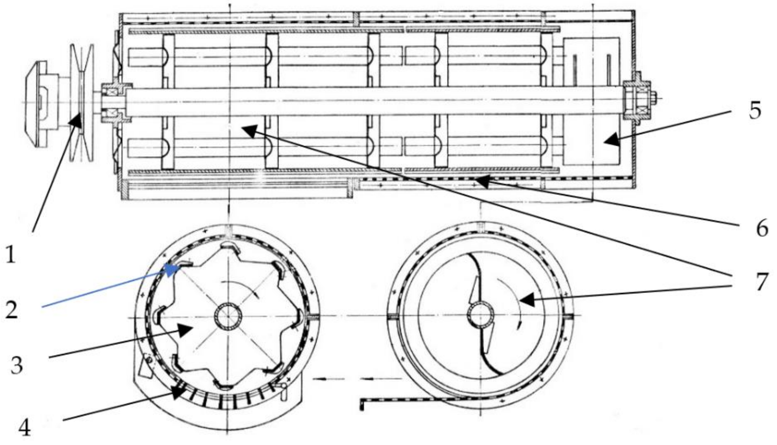
- Rotor speed n, adjustable within 620–1320 rpm; corresponding to this speed range, the peripheral speed of the rotor was in the range of 19.5–41.46 m·s−1;
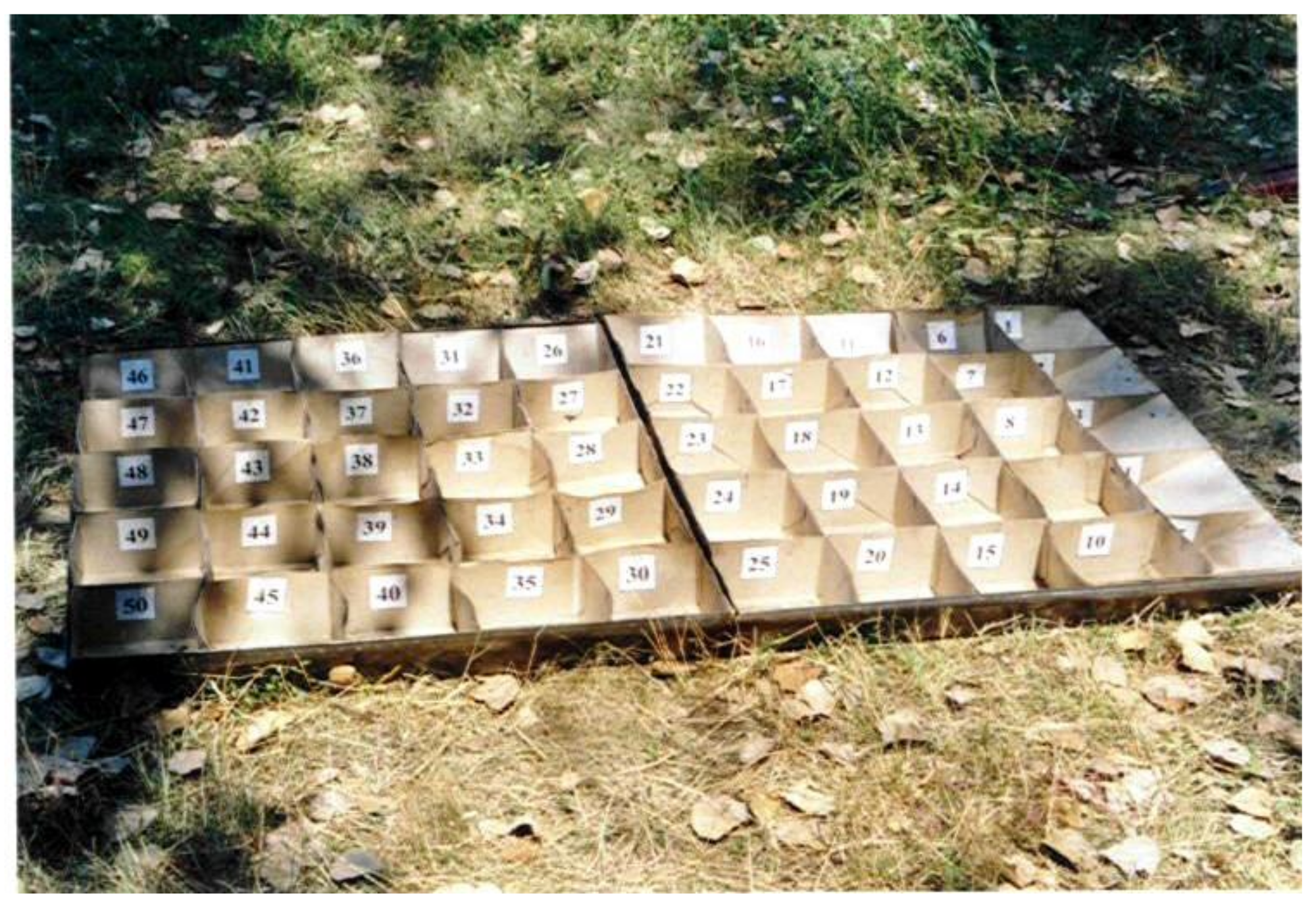
- Material flow q [kg·s−1], was determined by weighing the plant material sample and the time when the uniform feeding of the threshing apparatus was achieved. The mass of material introduced into the apparatus was verified for each test with the mass of the components collected following the threshing process. During tests, the material flow corresponding to the threshing apparatus width was modified in the limits 0.5–4.0 kg·s−1, the combine having a maximum material flow of 5–6 kg·s−1;
- The distance δ between the rotor’s rails and the counter-rotor is adjustable, measured in the direction of forwarding of the material. It can be varied thus: δi = 12–29 mm at the entrance and δe = 3–7 mm at exit;
- The material feed rate was varied within the limits: 0.06–0.50 m·s−1;
- The material feed angle can vary within limits: 0–15°.
- Peripheral speed of the rotor vp: 38–41 m·s−1
3. Results
3.1. Applying the Similarity Theory to Model the Threshing and Separation Process
- Q—material flow [kg·s−1];
- n—rotor speed [rpm];
- δ—distance between rotor and counter-rotor [m];
- ρ—mean density of the processed material [kg·m−3];
- va—feeding speed [m·s−1];
- Lt—length of the threshing apparatus [m];
- i—seeds/straws ratio [−];
- D—rotor diameter [m].
3.2. Considerations on The Density Function and the Probability Distribution of the Material Separated through the Space between Rotor and Counter-Rotor
- (1)
- Using the experimental data to determine the free parameter “A” so that the distribution function Ss to model the experimental data “as well as possible”, then to determine the dependence of this parameter on the process variables that appear in the argument list of the function F, for example in Equation (18); A is a parameter that will be calculated by any process taking into account certain conditions of the process: .
- (2)
- Considering the shape of the experimental curves, it is noted that the function Sd generally has a global extremum in the working range [0, L], reference point for the experiment, and this model can be imposed on the modeling function, with some additional conditions.
3.3. Functions of Distribution (Ss) and Distribution Density (Sd) of Separated Seeds
3.4. The Link between Ss and Sd Functions and the Experimental Results
3.5. Determination of the Other Functions’ Characteristic of the Threshing and Separation Process
3.6. Solving of the Problem if a Type (50) Relation Is Accepted
4. Conclusions
Author Contributions
Funding
Institutional Review Board Statement
Informed Consent Statement
Data Availability Statement
Acknowledgments
Conflicts of Interest
References
- Ali, K.A.M.; Huang, X.; Zong, W.; Abdeen, M.A.M. Mechanical structure and operating parameters of sunflower harvesting machines: A review. Int. Agric. Eng. J. 2020, 29, 143–153. [Google Scholar]
- Fu, J.; Chen, Z.; Han, L.; Ren, L. Review of grain threshing theory and technology. Int. J. Agric. Biol. 2018, 11, 12–20. [Google Scholar] [CrossRef]
- Li, Y.; Tao, C.; Zhe, Q.; Kehong, L.; Xiaowei, Y.; Dandan, H.; Dongxing, Z. Development and application of mechanized maize harvesters. Int. J. Agric. Biol. 2016, 9, 15–28. [Google Scholar] [CrossRef]
- Kumar, A.; Kumar, A.; Khan, K.; Kumar, D. Performance evaluation of harvesting and threshing methods for wheat crop. Int. J. Pure App. Biosci 2017, 5, 604–611. [Google Scholar] [CrossRef]
- Cujbescu, D.; Găgeanu, I.; Iosif, A. Mathematical modeling of ear grain separation process depending on the length of the axial low threshing apparatus. INMATEH-Agric. Eng. 2021, 65, 101–110. [Google Scholar] [CrossRef]
- Zhang, S.Z.; Yuzhong, H. Design and test of backpack harvester for sunflowers. J. Mech. Des. 2018, 35, 67–71. [Google Scholar]
- Siebenmorgen, T.J.; Andrews, S.B.; Vories, E.D.; Loewer, D.H. Comparison of combine grain loss measurement techniques. Appl. Eng. Agric. 1994, 10, 311–315. [Google Scholar] [CrossRef]
- Kepner, R.A.; Roy, B.; Barger, E.L. Principles of Farm Machinery, 2nd ed.; The AvI Publishing Company Inc.: Westport, CT, USA, 1982; pp. 86–88. [Google Scholar]
- Humburg, D.S.; Nicolai, R.E.; Reitsma, K.D. Best Management Practices for Corn Production in South Dakota; South Dakota State University: Brookings, SD, USA, 2009. [Google Scholar]
- Sumner, P.E.; Williams, E.J. Measuring Field Losses from Grain Combines. 2009. Available online: https://secure.caes.uga.edu/extension/publications/files/pdf/B%20973_3.PDF (accessed on 13 March 2022).
- Ali, K.A.M.; Zong, W.; Md-Tahir, H.; Ma, L.; Yang, L. Design, simulation and experimentation of an axial flow sunflower-threshing machine with an attached screw conveyor. Appl. Sci. 2021, 11, 6312. [Google Scholar] [CrossRef]
- Chavoshgoli, E.; Abdollahpour, S.; Ghassemzadeh, H. Designing, fabrication and evaluation of threshing unit edible sunflower. Agric. Eng. Int. CIGR J. 2019, 21, 52–58. [Google Scholar]
- Mirzabe, A.H.; Chegini, G.R.; Khazaei, J.; Massah, J. Design, construction and evaluation of preliminarily machine for removing sunflower seeds from the head using air-jet impingement. Agric. Eng. Int. CIGR J. 2014, 16, 294–302. [Google Scholar]
- Goel, A.; Behera, D.; Swain, S.; Behera, B. Performance evaluation of a low-cost manual sunflower thresher. Indian J. Agric. Res. 2009, 43, 37–41. [Google Scholar]
- Ashwini, T.; Vikas, L. Effect of moisture content on the physical properties of sunflower seeds (Helianthus annuus L.) for development of power-operated sunflower seed decorticator. Int. J. Sci. Res. 2014, 3, 2298–2302. [Google Scholar]
- Di, Z.; Cui, Z.; Zhang, H.; Zhou, J.; Zhang, M.; Bu, L. Design and experiment of rasp bar and nail tooth combined axial flow corn threshing cylinder. Trans. Chin. Soc. Agric. Eng. 2018, 34, 28–34. [Google Scholar]
- Miu, P.I.; Kutzbach, H.-D. Modeling and simulation of grain threshing and separation in threshing units—Part I. Comput. Electron. Agric. 2008, 60, 96–104. [Google Scholar] [CrossRef]
- El-Shal, M.S.; El-Ashry, A.S.; El-Shal, A.M.; Fakhrany, W.B. Development of a rubbing thresher for some seed crops. Misr. J. Agric. Eng. 2014, 31, 133–154. [Google Scholar] [CrossRef]
- Chansrakoo, W.; Chuan-Udom, S. Factors of operation affecting performance of a short axial-flow soybean threshing unit. Eng. J. 2017, 22, 109–122. [Google Scholar] [CrossRef]
- Chuan-Udom, S.; Chinsuwan, W. Threshing unit losses prediction for Thai axial flow rice combine harvester. Ama Agric. Mech. Asia Afr. Lat. Am. 2009, 40, 50–54. [Google Scholar]
- Srison, W.; Chuan-Udom, S.; Saengprachatanarug, K. Effects of operating factors for an axial-flow corn shelling unit on losses and power consumption. Agric. Nat. Resur. 2016, 50, 421–425. [Google Scholar] [CrossRef]
- Gummert, M.; Kutzbach, H.D.; Muhlbauer, W.; Wacker, P.; Quick, G.R. Performance evaluation of an IRRI axial-flow paddy thresher. AMA Agric. Mech. Asia Afr. Lat. Am. 1992, 23, 47–58. [Google Scholar]
- Saeng-Ong, P.; Chuan-Udom, S.; Saengprachatanarug, K. Effects of guide vane inclination in axial shelling unit on corn shelling performance. Agric. Nat. Resour. 2015, 49, 761–771. [Google Scholar]
- Alizadeh, M.R.; Khodabakhshipour, M. Effect of threshing drum speed and crop moisture content on the paddy grain damage in axial flow thresher. Cercet. Agron. Mold. 2010, 3, 5–11. [Google Scholar]
- Adekanye, T.A.; Osakpamwan, A.B.; Osaivbie, I.E. Evaluation of soybean threshing machine for small scale farmer. Agric. Eng. Int. CIGR J. 2016, 18, 426–434. [Google Scholar]
- Zaalouk, A.K. Evaluation of local machine performance for threshing bean. Misr J. Agric. Eng. 2009, 26, 1696–1709. [Google Scholar] [CrossRef]
- Vejasit, A.; Saengsit, W.; Kraisin, K.; Nuntasukol, S.; Sutthiwaree, P.; Samran, S. The Development and Testing of Rice Thresher for Soybean Seed Production; Full Report; Department of Agriculture: Bangkok, Thailand, 2005. [Google Scholar]
- Pholpo, T.; Sirisomboon, P.; Pholpo, K. Design and development of thresher of the small soybean harvester. In Proceedings of the 10th Thai Society of Agricultural Engineering International Conference, Bangkok, Thailand, 17–19 March 2017; pp. 175–179. [Google Scholar]
- Rembold, F.; Hodges, R.; Bernard, M.; Knipschild, H.; Léo, O. The African Postharvest Losses Information System (APHLIS): An Innovative Framework to Analyse and Compute Quantitative Postharvest Losses for Cereals under Different Farming and Environmental Conditions in East and Southern Africa; University of Greenwich: London, UK, 2011. [Google Scholar]
- Bansal, N.K.; Agarwal, S.; Sharma, T.R. Performance evaluation of a sunflower thresher. In The XXIX Annual Convention of India Society of Agricultural Engineering; India Society of Agricultural Engineering: Delhi, India, 1994. [Google Scholar]
- Sudajan, S.; Salokhe, V.M.; Chusilp, S. Effect of concave hole size, concave clearance and drum speed on rasp-bar drum performance for threshing sunflower. AMA Agric. Mech. Asia Afr. Lat. Am. 2005, 36, 52–60. [Google Scholar]
- Ismail, Z.E.; Elhenaway, M.N. Optimization of machine parameters for a sunflower thresher using friction drum. J. Agric. Sci. Mansoura Univ. 2009, 34, 10293–10304. [Google Scholar]
- Miu, P. Modeling of the Threshing Process at Grain Harvesters. Ph.D. Thesis, University Politehnica of Bucharest, Bucharest, Romania, 1995. [Google Scholar]
- Bosoi, E.S.; Verniaev, O.V. Teoria, Construkţia i Rascent Selsko-Hoziaistvenîh Maşin’; Maşinostroenie: Moskva, Russia, 1978; pp. 334–339. [Google Scholar]


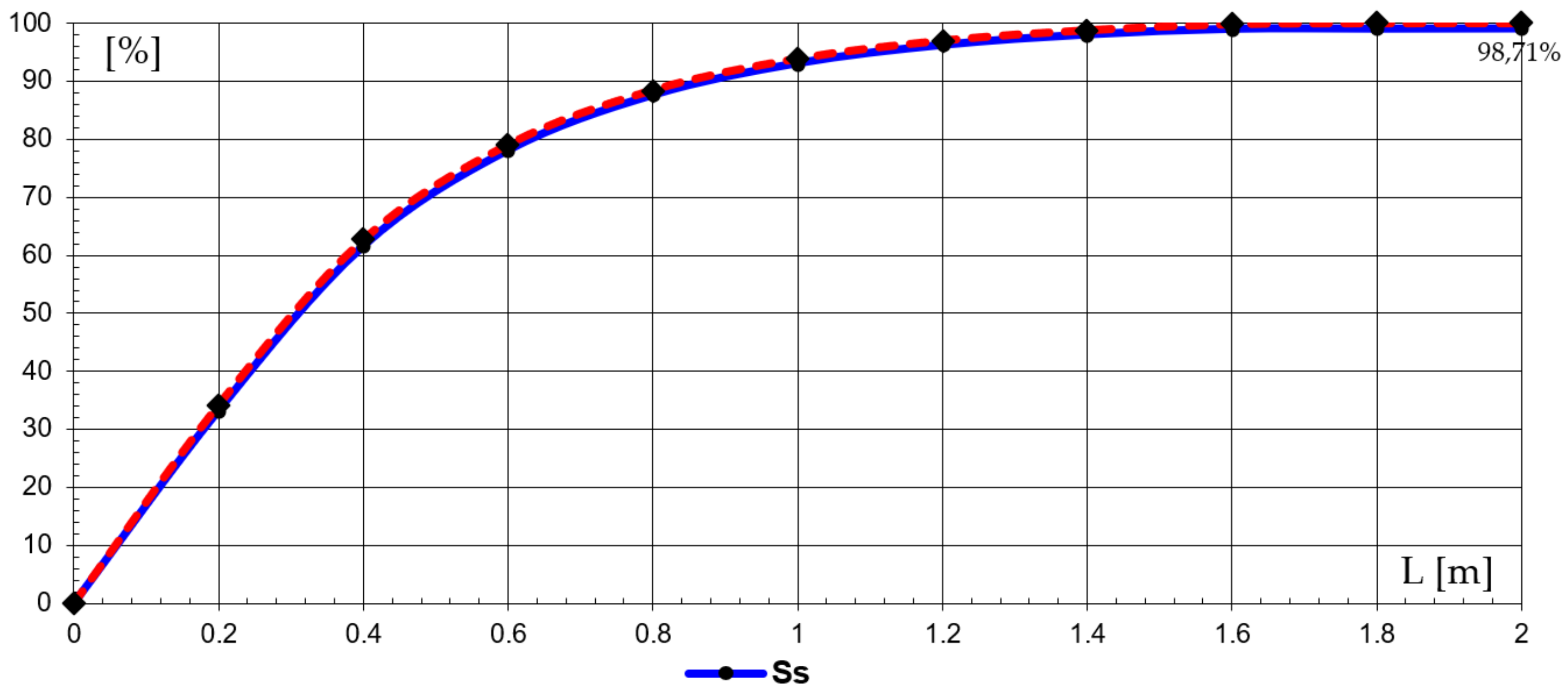
 curve drawn by points;
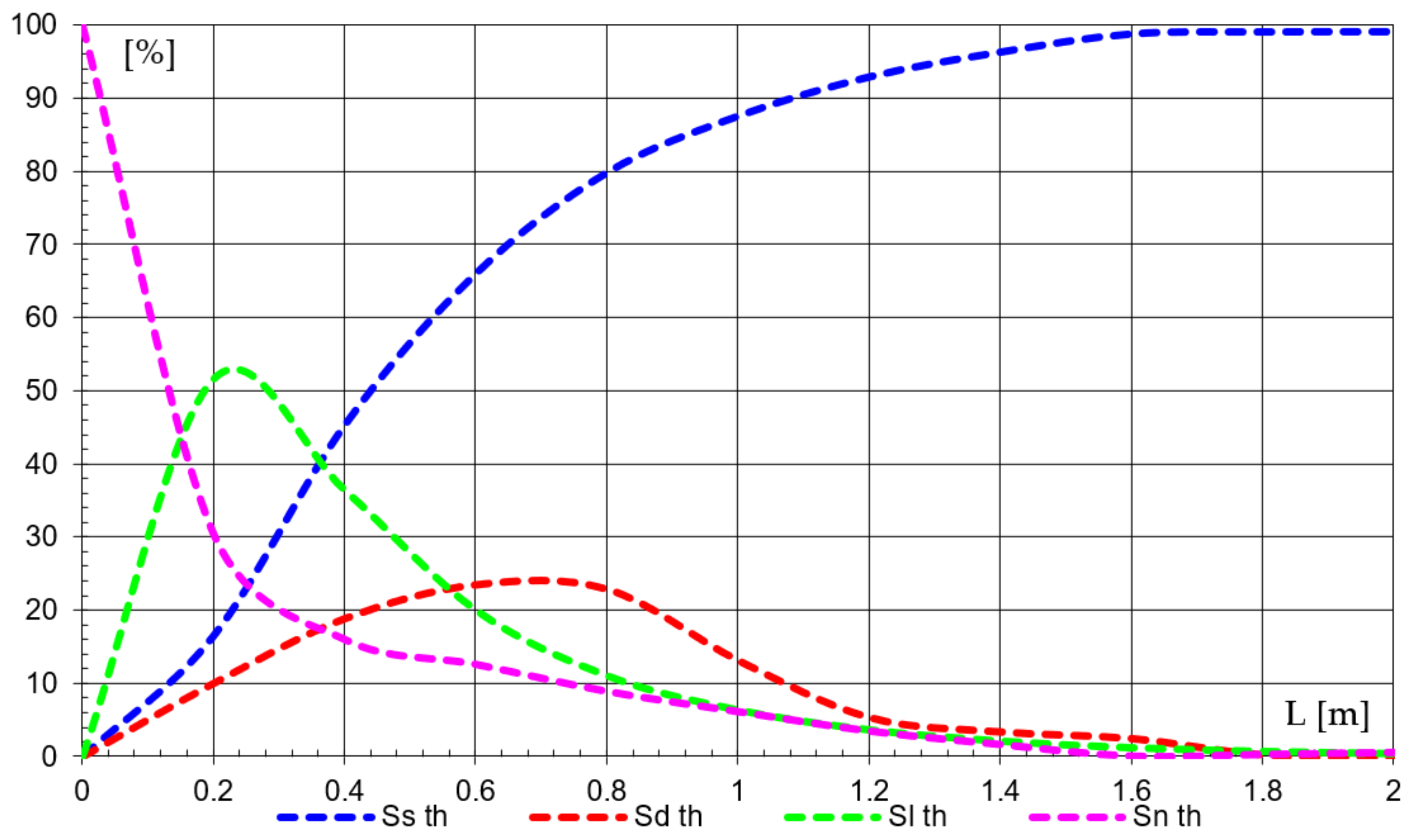
  theoretical curve).
curve drawn by points; theoretical curve).
theoretical curve).
curve drawn by points; theoretical curve). curve drawn by points; theoretical curve).
curve drawn by points; theoretical curve).
curve drawn by points; theoretical curve).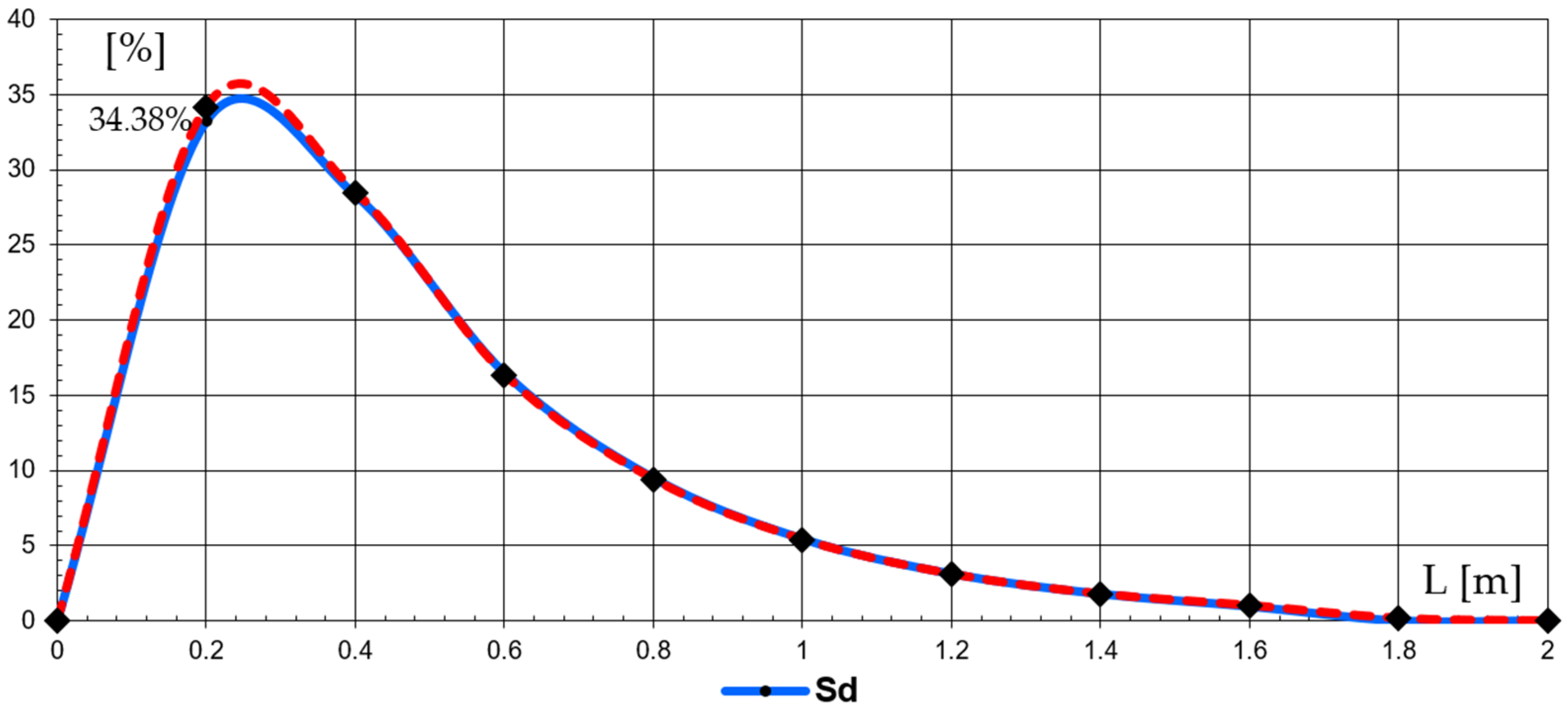
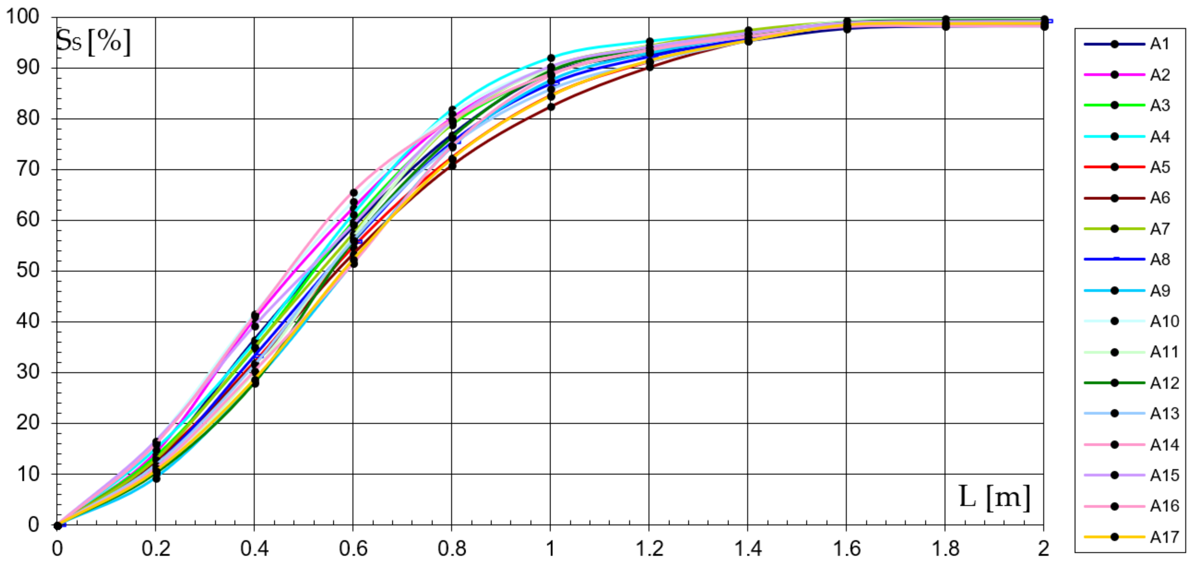
 curve drawn by points).
curve drawn by points).
curve drawn by points).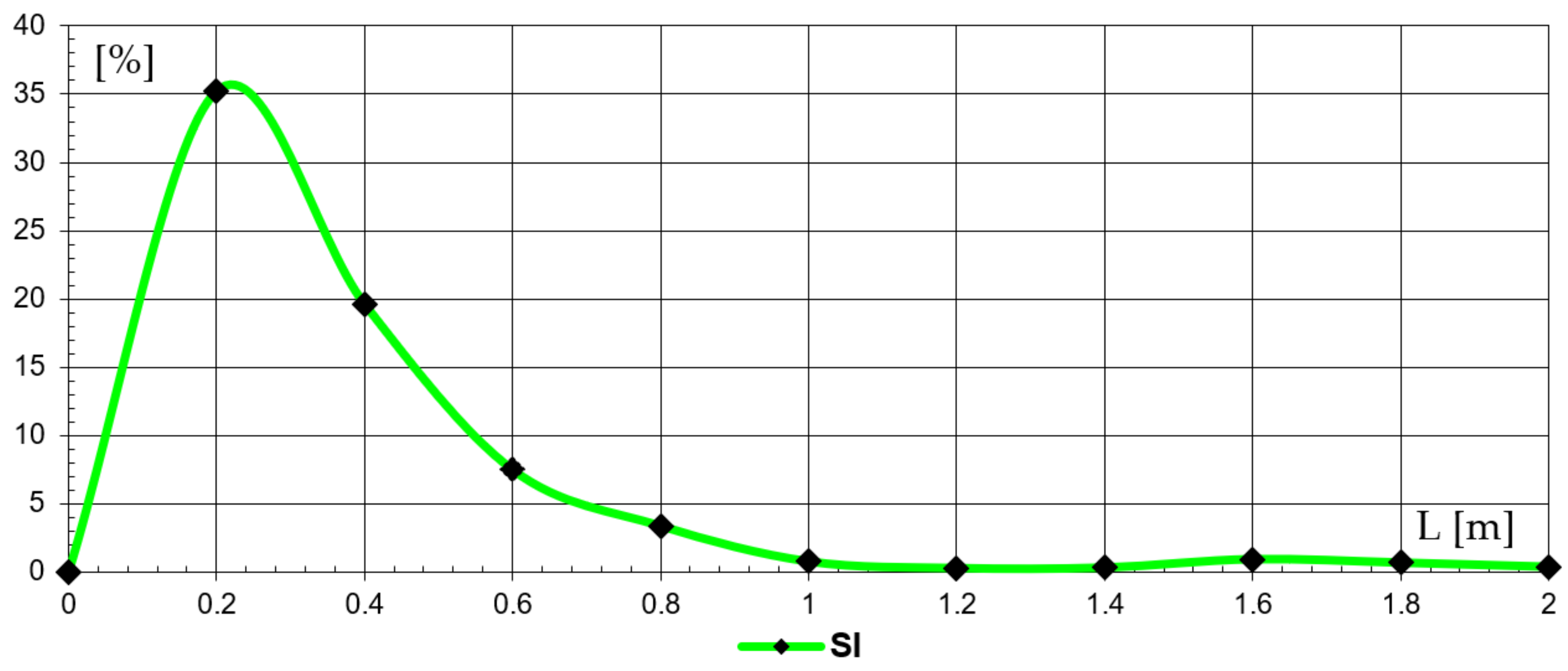
 curve drawn by points).
curve drawn by points).
curve drawn by points).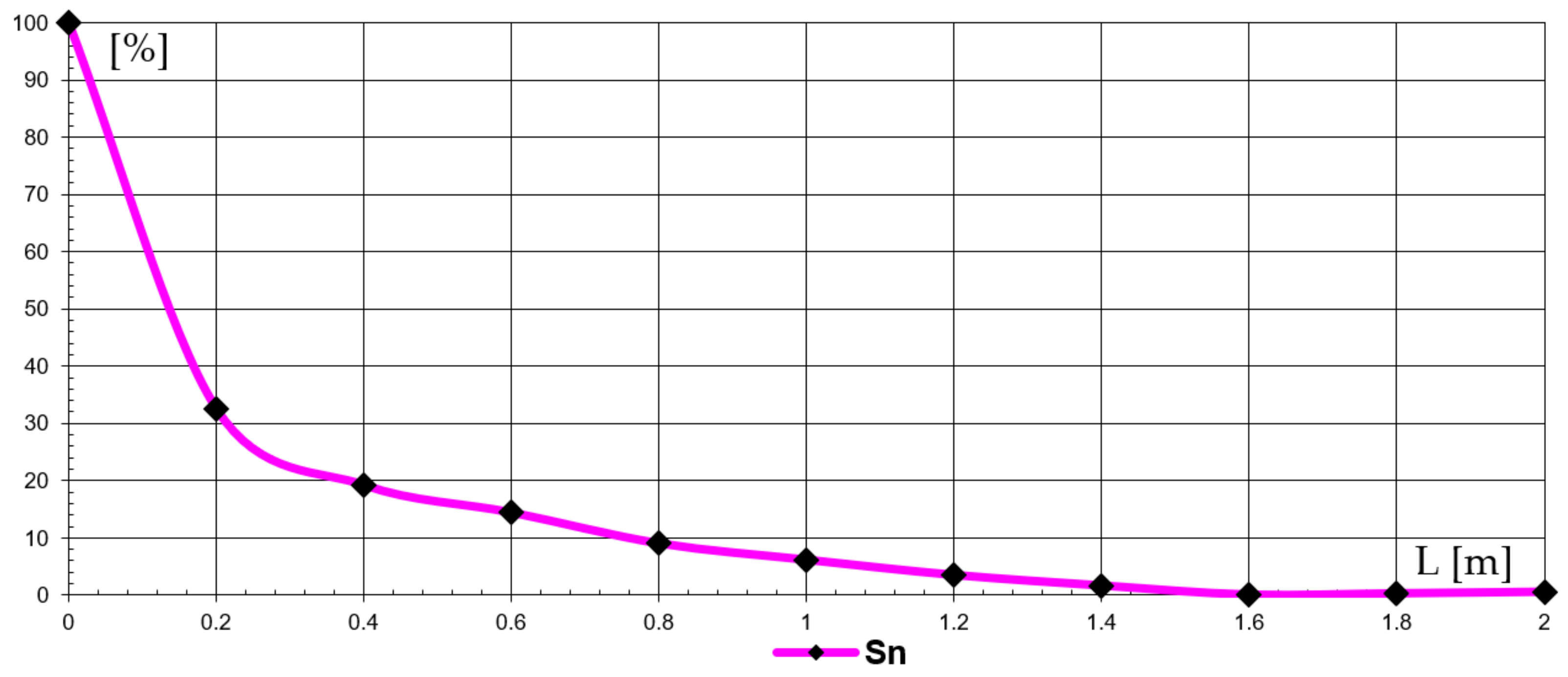


| No. | Parameter | Exponent L (Length) | Exponent M (Mass) | Exponent T (Time) |
|---|---|---|---|---|
| 1 | λ | −1 | 0 | 0 |
| 2 | n | 0 | 0 | −1 |
| 3 | δ | 1 | 0 | 0 |
| 4 | va | 1 | 0 | −1 |
| 5 | ρ | −3 | 1 | 0 |
| 6 | L | 1 | 0 | 0 |
| 7 | Q | 0 | 1 | −1 |
| 8 | SS | 0 | 1 | 0 |
| 9 | pev | 0 | 1 | 0 |
| No. | Parameter | Dispersion Dλ |
|---|---|---|
| 1 | 0.20700013 | |
| 2 | 0.22533057 | |
| 3 | 0.16572981 | |
| 4 | 0.17762885 | |
| 5 | 0.18200157 | |
| 6 | 0.15471791 | |
| 7 | 0.15722568 | |
| 8 | 0.16040659 | |
| 9 | 0.17687420 | |
| 10 | 0.15757224 | |
| 11 | 0.14328398 | |
| 12 | 0.15254997 | |
| 13 | 0.15693625 | |
| 14 | 0.15396032 | |
| 15 | 0.14783308 | |
| 16 | 0.12690374 |
Publisher’s Note: MDPI stays neutral with regard to jurisdictional claims in published maps and institutional affiliations. |
© 2022 by the authors. Licensee MDPI, Basel, Switzerland. This article is an open access article distributed under the terms and conditions of the Creative Commons Attribution (CC BY) license (https://creativecommons.org/licenses/by/4.0/).
Share and Cite
Vlăduț, N.-V.; Biriş, S.-Ş.; Cârdei, P.; Găgeanu, I.; Cujbescu, D.; Ungureanu, N.; Popa, L.-D.; Perişoară, L.; Matei, G.; Teliban, G.-C. Contributions to the Mathematical Modeling of the Threshing and Separation Process in An Axial Flow Combine. Agriculture 2022, 12, 1520. https://doi.org/10.3390/agriculture12101520
Vlăduț N-V, Biriş S-Ş, Cârdei P, Găgeanu I, Cujbescu D, Ungureanu N, Popa L-D, Perişoară L, Matei G, Teliban G-C. Contributions to the Mathematical Modeling of the Threshing and Separation Process in An Axial Flow Combine. Agriculture. 2022; 12(10):1520. https://doi.org/10.3390/agriculture12101520
Chicago/Turabian StyleVlăduț, Nicolae-Valentin, Sorin-Ştefan Biriş, Petru Cârdei, Iuliana Găgeanu, Dan Cujbescu, Nicoleta Ungureanu, Lorena-Diana Popa, Lucian Perişoară, Gheorghe Matei, and Gabriel-Ciprian Teliban. 2022. "Contributions to the Mathematical Modeling of the Threshing and Separation Process in An Axial Flow Combine" Agriculture 12, no. 10: 1520. https://doi.org/10.3390/agriculture12101520
APA StyleVlăduț, N.-V., Biriş, S.-Ş., Cârdei, P., Găgeanu, I., Cujbescu, D., Ungureanu, N., Popa, L.-D., Perişoară, L., Matei, G., & Teliban, G.-C. (2022). Contributions to the Mathematical Modeling of the Threshing and Separation Process in An Axial Flow Combine. Agriculture, 12(10), 1520. https://doi.org/10.3390/agriculture12101520