Abstract
In the last decades, farm animals kept in confined and mechanically ventilated livestock buildings have been increasingly confronted with heat stress (HS) due to global warming. These adverse conditions cause a depression of animal health and welfare and a reduction of the performance up to an increase in mortality. To facilitate sound management decisions, livestock farmers need relevant arguments, which quantify the expected economic risk and the corresponding uncertainty. The economic risk was determined for the pig fattening sector based on the probability of HS and the calculated decrease in gross margin. The model calculation for confined livestock buildings showed that HS indices calculated by easily available meteorological parameters can be used for assessment quantification of indoor HS, which has been difficult to determine. These weather-related HS indices can be applied not only for an economic risk assessment but also for weather-index based insurance for livestock farms. Based on the temporal trend between 1981 and 2017, a simple model was derived to assess the likelihood of HS for 2020 and 2030. Due to global warming, the return period for a 90-percentile HS index is reduced from 10 years in 2020 to 3–4 years in 2030. The economic impact of HS on livestock farms was calculated by the relationship between an HS index based on the temperature-humidity index (THI) and the reduction of gross margin. From the likelihood of HS and this economic impact function, the probability of the economic risk was determined. The reduction of the gross margin for a 10-year return period was determined for 1980 with 0.27 € per year per animal place and increased by 20-fold to 5.13 € per year per animal place in 2030.
1. Introduction
Livestock production is threatened by various effects of global warming such as availability of feed and pasture, reduction in feed yield from drought [1,2,3], health aspects [4], new diseases, new transmitting vectors [5,6,7,8,9,10] and heat stress (HS). For pig and poultry, which are frequently kept inside confined livestock buildings, HS is often higher indoor than outdoor due to the release of sensible and latent heat of the animals [11]. In a warmer climate, HS may become, therefore, one of the major threats for conventional, intensive pig and poultry production [12]. The main aims of this investigation are (1) the quantification of increase of HS in Central Europe since 1981 with a future perspective up to 2030, and (2) the estimation of the increase of economic risk for pig farms for the same region and time period. The analysis aims to answer the following research questions. (1) How can weather-related HS indices be used in an economic risk assessment? (2) What is the impact of global warming on the likelihood of weather-related HS indices in Central Europe? (3) What is the economic impact of global warming-related HS on fattening pigs? (4) What can we learn, including conceptual uncertainties, from this analysis for other locations and production systems? Overall, answers to these questions are relevant for farmers who require information on the likelihood and severity of future HS specific for farm animals in order to plan for adaptation measures for existing farms or when investing in new livestock housing.
Several investigations have stresses the importance of this issue. For sows Bjerg, et al. [13] showed that feed intake, milk yield, body weight loss during lactation, mortality, litter, daily weight gain during lactation and sow behavior had a strong dependence on ambient temperature. For fattening pigs an optimal ambient temperature in the range between 15 °C and 23 °C was found for the optimum daily gain and feed efficiency [14]. Most of the investigations showed a nonlinear relationship between ambient temperature and physiological parameters for pig and poultry with progressive effects for increasing HS [14,15,16,17]. The economic consequences of HS are related to the feeding costs, which are caused by the average daily gain and feed conversion ratio, because the feeding costs are a major part of the variable production costs and the related gross margin. However, more severe effects like mortality are HS-related as well [18,19,20,21,22,23].
A common measure of the risk associated with a specific environmental situation is the product of the likelihood of this situation and its impact. Focusing on only one of these two factors, or considering them only sequentially, is insufficient. For a proper risk assessment, the interaction between them both matters. King, et al. [24] pointed out that there are several problems and shortfalls of quantitatively characterizing risks. Inadequate quantifications are caused by a high sensitivity to uncertainties and incomplete assumptions. They are also likely to be systematically biased towards underestimation of risk, as they tend to omit a wide range of impacts that are difficult to quantify. The authors emphasized that risks should always be assessed in relation to objectives of analysis. In the case of climate change and confined livestock keeping of pigs and poultry, one of the relevant objectives is related to the evaluation and the application of adaptation measures to cope with undesirable weather impacts [25,26,27,28,29].
The increase in the frequency of hot days and heat waves in recent decades, due to global warming, has increased the likelihood of the situations that cause HS [30,31,32,33,34,35]. The likelihood of the occurrence of a certain HS index can be quantified by a probability density function, which is defined by the temporal trend (caused by global warming) and a stochastic component [35].
The reaction of animals to the occurrence of HS is partly known for several output traits of livestock production, which impact both variable costs or the revenue (e.g., average daily gain, feed conversion ratio, milk yield, egg production (number and mass), water demand, farrowing rate, litter size, meat quality and mortality). A main challenge is to find an appropriate mathematical function with a certain HS index as a predictor for such traits. For this paper we derived an impact function on the dataset of St-Pierre et al. [36] and used it to quantify the economic risk of increased HS. Toeglhofer et al. [37] analyzed the economic risk due to HS by applying the weather-value-at-risk (weather-VaR) concept. They adapted the VaR concept as an economic risk measure of the maximum potential loss within a given confidence interval, which is determined by the weather. In this article, we use the weather-VaR to describe the economic risk of heat stress on the gross margin of fattening pigs. We assume changes in gross margins as an appropriate measure for economic risks since we do not consider investment decisions (e.g., adaptation) but analyze the economic impacts from adverse weather events.
This paper is structured in three steps. In the first step, the likelihood of heat stress is calculated by the use of a simulation model for a confined livestock building, which is driven by meteorological data. The stochastic element of the weather is the major input for the uncertainty from year to year. The calculated heat stress parameters are available over the last 37 years, which results in the likelihood for heat stress for certain years. In a second step, the impact of heat stress on the gross margin is calculated modifying the impact function of St-Pierre, Cobanov and Schnitkey [36]. In the last step, the likelihood of heat stress and the impact function are combined to determine the likelihood of the economic risk on the basis of the weather-VaR concept for the reduction of the gross margin per animal place.
The assessment of the economic risk for confined livestock due to HS is demonstrated for a pig fattening operation located in Central Europe. The analysis is based on the simulation of the indoor climate inside a reference livestock building for fattening pigs [11]. The likelihood of HS is used to quantify the economic risk of these environmental constraints.
2. Materials and Methods
2.1. Likelihood of HS Inside Livestock Builings
The likelihood of HS is determined by a simulation model of the indoor climate of a confined livestock building, which is driven by meteorological data, directly measured at the site of investigation, the city of Wels in Upper Austria (48.16° N, 14.07° E) for the period 1981 to 2017 with a temporal resolution of one hour, and based on climate simulations for the surrounding area representative for class Cfb (warm temperature, fully humid, warm summers) following the climate classification of Köppen and Geiger [38]. The data were provided by the Austrian Meteorological Service ZAMG (Zentralanstalt für Meteorologie und Geodynamik, Vienna, Austria).
The indoor climate of the livestock building was simulated by a steady-state model, which calculates the thermal indoor parameters (air temperature and humidity) and the ventilation flow rate. The thermal environment inside the building depends on the livestock, the thermal properties of the building, the ventilation system, and its control unit. The core of the model is the calculation of the sensible heat balance of a livestock building [11,39,40]. The model calculation was performed for a typical livestock building for fattening pigs in Central Europe for 1800 head, divided into nine sections with 200 animals each. The system parameters, which describe the conventional reference system (properties of the livestock, building, and the mechanical ventilation system), are summarized in Table 1. The model calculations were performed for the entire growing-fattening period for a body mass between 30 and 120 kg. The investigation period covered the years from 1981 to 2017.

Table 1.
System parameters for livestock, building, and ventilation system related to one animal place for the indoor climate simulation of a conventional livestock building [11].
Two parameters quantify HS for farm animals: (1) the (dry bulb) air temperature T, and (2) the temperature-humidity index THI = 0.72 T + 0.72 TWB + 40.6, where TWB represents the wet bulb temperature. For a certain threshold X, the exceedance frequency PX and the intensity of HS AX, using the aggregated values between X and the time course of the HS index (i.e., the area under the time course), were calculated. PX (h a−1) gives the number of hours per year during by which the selected threshold is exceeded, AX (Kh a−1 for temperature and h a−1 for THI) includes the differences of the instantaneous values and the threshold. Two threshold values were selected for fattening pigs: the temperature X = 25 °C and the THI X = 75, which presents an alert situation of the thermal environment [42]. These two thresholds resulted in four HS indices PT25, AT25, PTHI75, and ATHI75. The HS indices were further processed as annual sums.
The four indices were calculated from indoor parameters based on a simulation of the thermal environment inside the livestock building, where the vector of IINT denotes for PT25, AT25, PTHI75, and ATHI75 inside the building. For the outdoor parameters, using meteorological measurements easily available from a nearby weather station, the vector IEXT denotes for PT25, AT25, PTHI75, and ATHI75.
To estimate the likelihood of the occurrence of a certain HS index for a certain year t, a simple model was fitted to the dataset. The model is characterized by the expected value It of a HS index of a certain year t and the variability s2. The expected value It is calculated by a linear regression of the logarithmically transformed HS index according to log It = kt + d, with the slope k and the intercept d. The deviation of the HS index from the linear trend It results in the variance s2. The detrended (and logarithmically transformed) HS indices, according to ΔEXT,t = log Tt – log IEXT,t (deviation from the trend) were fitted to the Weibull, the Gumbel, and the Gauss (normal) distributions. The quality of the fit was determined by the Akaike information criterion AIC.
The trends of the HS indices [11] were tested by the signal-to-noise ratio (SNR) and the Mann-Kendall Trend Test. The signal-to-noise ratio SNR was calculated using a linear trend over 37 years and the standard deviation of the annual mean values of the HS indices. Under the assumption, that the SNR is distributed with the standard normal distribution (0; 1), limits for the SNR and the p-values are as follows [43]: low significance 1.645 < SNR ≤ 1.960 (0.05 < p ≤ 0.10), medium significance 1.960 < SNR ≤ 2.576 (0.01 < p ≤ 0.05) and high significance SNR > 2.576 (p ≤ 0.01). The second test for the trend of the HS indices was the rank-based nonparametric Mann-Kendall trend test with the test statistic τ and a one-sided test for an increasing temporal trend using the R package trend.
The fitting of empirical data by a selected distribution function was performed by a maximum likelihood estimation. The goodness of the fit was evaluated by the Akaike information criteria AIC.
The variability of the HS indices ΔEXT was tested by the Breusch-Pagan test for heteroskedasticity, assuming that the residuals ΔEXT are normally distributed. Using a χ2 test, it was tested whether the variance of the errors from the regression depends on the values of the independent variable, the time t.
The relationship between the two vectors of HS indices (IINT and IEXT) was investigated by a linear regression analysis, using the model calculations by Mikovits, Zollitsch, Hörtenhuber, Baumgartner, Niebuhr, Piringer, Anders, Andre, Hennig-Pauka, Schönhart and Schauberger [11] for the indoor related vector IINT = [PT25, AT25, PTHI75, ATHI75] and the corresponding vector IEXT = [PT25, AT25, PTHI75, ATHI75], calculated by the outdoor (meteorological) parameters. The linear regression was evaluated by the p-value of the coefficient of determination r2.
2.2. Economic Impact of HS
The economic impact assessment was based on the reduction of the gross margin as a function of HS, estimated by the growing-fattening pig model of St-Pierre, Cobanov and Schnitkey [36]. The reduction of the gross margin was calculated by three parameters on an annual basis for one animal place: the reduction of body mass at the end of the fattening period (kg a−1) (revenue), the reduction of dry matter intake (kg a−1) (variable costs) and the increase of mortality (%) (revenue). These three parameters were updated by data for 2020 from the Federal Institute of Agricultural Economics (AWI http://www.awi.bmnt.gv.at/) for feed at 0.25 € kg−1, the revenue for a fattening pig at 1.7 € kg−1, and the cost of a slaughtered pig (75 kg) at 100 €. The original predictor of the impact function for growing-fattening pigs of St-Pierre, Cobanov and Schnitkey [36] is the area under the curve AX for a THI threshold of X = 72. By the dataset of the HS index using the two THI thresholds, X = 72 (growing-fattening pigs) and X = 74 (sows), the impact function was modified for the THI threshold X = 75 used in this paper.
The economic impact IMP (€ a−1) related to one animal place as a linear function of the HS index ATHI75 (h a−1) reads as follows: IMP = 0.0016 ATHI75 with r2 = 0.9897 (Figure 1).
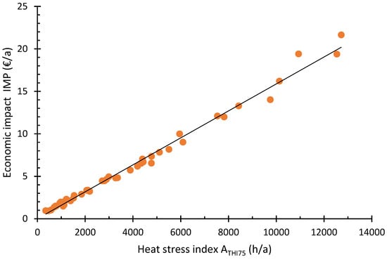
Figure 1.
Economic impact IMP (€/a per animal place), described by the reduction of the gross margin per animal place as a linear function of the heat stress index ATHI75 (h/a) derived from St-Pierre, Cobanov and Schnitkey [36] with IMP = 0.0016 ATHI75.
3. Results
3.1. Relationship between Indoor-Related and Weather-Related Heat Stress Indices
To assess the risk caused by HS inside confined livestock buildings, indoor parameters like air temperature and the temperature-humidity index THI should be the first choice. The disadvantage in using these parameters is the complex dependencies between indoor and outdoor (meteorological) parameters due to the thermal properties of the building, the ventilation system and its interaction with the livestock, which leads to intricate mathematical models associated with long computing times. The relationship between the vector of HS indices IINT = [PT25, AT25, PTHI75, ATHI75], calculated by indoor parameters, and the vector of HS indices IEXT = [PT25, AT25, PTHI75, ATHI75], calculated by the outdoor (meteorological) parameters, shows a high linear correlation. The statistical parameters of the linear regression are summarized in Table 2 and graphically presented in Figure 2. All HS indices of the vector IEXT = [PT25, AT25, PTHI75, ATHI75] show a high explanatory power for the indoor-related vector IINT = [PT25, AT25, PTHI75, ATHI75], explaining more than 80% of the variance (r2 > 0.80, p < 0.001) in each case. The intercept of the regression can be interpreted as the impact resulting from an increase of the indoor temperature and indoor humidity by the sensible and latent heat release of the farm animals. The slope of the two exceedance frequencies PT25 and PTHI75 are closer to the line of identity (1:1) compared to the HS intensities AT25 and ATHI75.
Table 2.
Linear regression results of vector IINT = [PT25, AT25, PTHI75, ATHI75] (calculated by the indoor parameters) as a function of the vector IEXT = [PT25, AT25, PTHI75, ATHI75] (calculated by weather data) with the coefficient of determination r2 of the linear regression with the slope k and the intercept d. The p-values are <0.001.
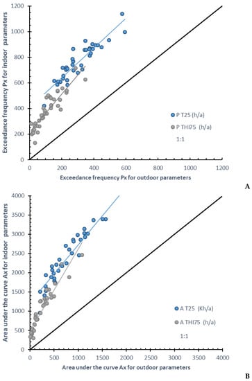
Figure 2.
Relationship between the weather-related vector of heat stress indices IEXT = [PT25, AT25, PTHI75, ATHI75] and the indoor-related vector of HS indices IINT = [PT25, AT25, PTHI75, ATHI75]. The exceedance frequencies of a threshold PT25 and PTHI75 (h/a) are presented in panel (A), the heat stress intensities (area under the curve for a threshold) AT25 (Kh/a) and ATHI75 (h/a) in panel (B). The parameters of the linear regression are summarized in Table 2.
Due to the reliable linear relationship between the two vectors of HS indices, shown by the high coefficient of determination (r2 > 0.80, p < 0.001) (Table 2), the vector of the HS indices IEXT= [PT25, AT25, PTHI75, ATHI75] can be used as a proxy to quantify the HS impact on farm animals without the need of a determination of the indoor parameters. This is an advantage for manageability, e.g., for weather-index based insurance, because the meteorological parameters are easily available from national weather services and no further model calculations are required.
3.2. Consequence of Global Warming on the Likelihood of Heat Stress Indices
The temporal trend of the weather-related vector of HS indices IEXT = [PT25, AT25, PTHI75, ATHI75] has been confirmed by the signal-to-noise ratio SNR and the Mann-Kendall trend test on a high level of significance with p < 0.04 and p <0.001, respectively (Table 3).
Table 3.
Statistical analysis of the temporal trend of the weather-related vector of heat stress (HS) indices IEXT = [PT25, AT25, PTHI75, ATHI75] by the signal-to-noise ratio SNR and the Mann-Kendall Trend Test with the test statistics τ with the corresponding p-values.
The simple model to estimate the expected likelihood of the occurrence of the HS indices of the vector IEXT = [PT25, AT25, PTHI75, ATHI75] for a certain year t was fitted by the empirical data to determine the expected value It and the variability s2. The expected value It of the distribution and the statistical parameters of the linear trend are given in Table 4. The results of all four weather-related HS indices of the vector IEXT show a high significance with p < 0.001 and a coefficient of determination r2 between 30% and 33%.
Table 4.
Temporal trend of the weather-related heat stress indices log It = kt + d, calculated by the logarithmically transformed heat stress indices log IEXT with the slope k, the intercept d, the coefficient of determination r2, and the p value.
The deviation of the HS indices from the linear trend results in the variance s2 showing a homoscedasticity of the four detrended HS indices ΔEXT, which was confirmed by the Breusch-Pagan test for all four weather-related HS indices of the vector IEXT = [PT25, AT25, PTHI75, ATHI75] at the 5% level. The detrended (and logarithmically transformed) HS indices were fitted to the Weibull distribution, the Gumbel distribution and the Gauss (normal) distribution. The last distribution showed the best overall fit, assessed by the Akaike information criterion AIC. In Table 5, the standard deviation s and the AIC are summarized. Figure 3 compares the empirically detrended (and logarithmically transformed) HS indices ΔEXT with the three fitted CDFs: Gauss, Weibull, and Gumbel distributions. Especially the right tail of the detrended HS indices ΔEXT is fitted well by the normal distribution.
Table 5.
Standard deviation s of the detrended (and logarithmically transformed) weather-related heat stress indices ΔEXT and the Akaike information criteria AIC.
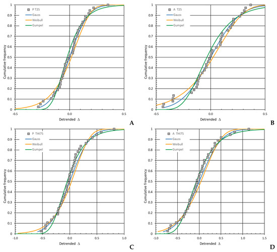
Figure 3.
Cumulative distribution of the detrended (and logarithmically transformed) heat stress indices ΔEXT and three cumulative distribution functions: Gauss, Weibull and Gumbel distribution for the four weather-related heat stress indices PT25 (A), AT25 (B), PTHI75 (C), and ATHI75 (D), describing the variability of HS.
These parsimonious models for the four HS indices of the vector IEXT = [PT25, AT25, PTHI75, ATHI75] were used to determine the likelihood of their occurrence in a certain year t. In Figure 4 the likelihood for the past (t = 1980 and t = 2020) and for the near future (t = 2030) is shown for the exceedance probability for PT25, and PTHI75 in panel A and the area under the curve AT25 and ATHI75 in panel B, using the cumulative distribution function (CDF) of the log-normal distribution.
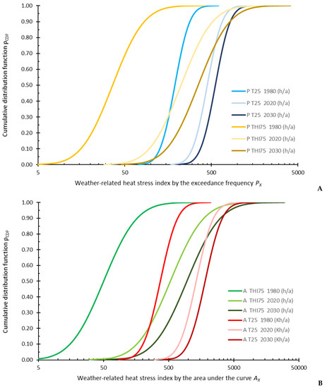
Figure 4.
Likelihood for the occurrence of the weather-related heat stress indices IEXT = [PT25, AT25, PTHI75, ATHI75] shown by the cumulative distribution function (CDF) of a log-normal distribution for t = 1980 (dark color), t = 2020 (light color), and t = 2030 (very dark color) for the exceedance frequency PT25, and PTHI75 (panel (A)) and the area under the curve AT25, and ATHI75 (panel (B)).
3.3. Consequence of Global Warming on Extreme Values of Heat Stress Indices
For economic risks, the temporal change of the likelihood of extreme values (right tail values of the curves in Figure 4) is an important aspect. For this analysis, we defined the extreme value by the 90-percentile (which corresponds to an exceedance probability PE of 10% and a return period of 10 years), according to the weather-VaR concept.
The extreme value Et,10% of each weather-related HS index was determined by the cumulative distribution function shown in Figure 4 for the year t = 1980 E1980,10% and for t = 2020 E2020,10% and by the 90-percentile of the CDF.
Based on PE = 10% the corresponding RP = 1/PE resulted in RP = 10 a (one in10-years event), as the length of an average time interval between the occurrences of two years with an HS level that exceeds the extreme value Et,10%.
For the time shift from 1980 to 2020, and for the near future from 2020 to 2030, the corresponding PE for t = 2020 and t = 2030 with PE,2020 and PE,2030 was calculated according to the temporal trend It (Table 4) and the standard deviation of the detrended values s (Table 5). The RP (in years) and PE,t are presented for the time shift in the past and for the time shift in the future in Table 6.
Table 6.
Exceedance probability PE and return period RP using the 90-percentile pCDF = 90% (PE = 10%) of the cumulative distribution function. The time shift was calculated for the past t = 1980 and t = 2020, and the near future t = 2020 and t = 2030. The shift of the mean values MV (expected value of the HS index for an exceedance probability of 50%) shows the consequence of global warming.
For weather-index-based insurance, a certain percentile of the CDF in Figure 5 (for example, 95-percentile, which means a 20-year return period) can be selected as a threshold to decide if the risk transfer mechanism becomes active and the insurance benefit is paid out.
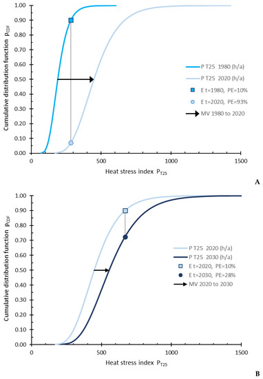
Figure 5.
The cumulative distribution function showing the likelihood of the occurrence of PT25. The shift of the mean value (pCDF = 0.5) is presented by the black arrow. In panel (A) the scenario of the past (t = 1980 and t = 2020) is shown, and in panel (B) the scenario of the near future (t = 2020 and t = 2030) is shown.
For four decades in the past (1980 to 2020), the return period was shortened from RP = 10 a in 1980 to about RP = 1 a, which means that the extreme value with an exceedance probability of 10% in 1980 can be expected every year in 2020. The mean values (MV) increased during the four decades between 136% (PT25) and 957% (ATHI75). In Figure 5A the scenario of the weather-related HS index PT25 is shown exemplarily for the past (t = 1980 and t = 2020). t = 1980, PE = 10% (pCDF = 90%) results in E1980,10% = 283 h/a (Table 7). Forty years later, the corresponding PE (t = 2020) is PE = 93%. This means, that the extreme value of the year t = 1980 E1980,10% = 283 h/a will be exceeded with a probability of 93% in 2020, or 13 a out of 14 a. The mean value is more than doubled from 190 h/a (in 1980) to 448 h/a 40 a later (Figure 5A).
Table 7.
Statistics of economic risk by the reduction of the gross margin (€ a−1) per animal place for t = 1980, t = 2020, and t = 2030. The weather-VaR values were calculated for a 90 and 95-percentile, corresponding to a return period of 10 a and 20 a, respectively.
For the next decade (2020 to 2030), the return period is shortened from RP = 10 a in 2020 to 3–4 a in 2030. An increase of about 24% (PT25) to 80% (ATHI75) of the mean value in relation to 2020 can be expected for the upcoming decade. In Figure 5B the likelihood of PT25 for the near future is shown. The exceedance probability PE = 10% (pCDF = 90%) in the year t = 2020 E2020,10% = 668 h/a is shifted for the year t = 2030 to PE = 28%. The mean value increases from 448 h/a to 556 h/a.
For both scenarios (past and near future), the increase of HS is much higher for the THI index (PTHI75 and ATHI75) compared to the temperature index (PT25 and AT25). This means that not only the air temperature, but also the humidity, which is part of the THI index, will increase with time. Otherwise, the temperature-based index would grow proportional to the THI index.
3.4. Economic Risk for Pig Farms due to Global Warming
The economic risk due to global warming was assessed by the product of the likelihood of HS (Figure 6) and the economic impact function, which describes the expected reduction of the gross margin as a function of the HS index ATHI75, shown in Figure 1.
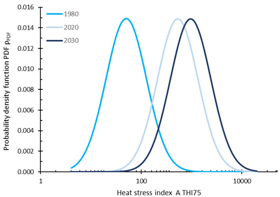
Figure 6.
Likelihood of the occurrence of the weather-related heat stress index ATHI75 for t = 1980, t = 2020, and t = 2030.
The likelihood of the weather-related HS index ATHI75 is shown by the probability density function (PDF) in Figure 6. It defines the temporal trend It which gives the expected value of the HS index for a certain year t (mean value (maximum) of the PDF) and the standard deviation s.
The economic risk due to global warming is shown by PDFs (Figure 7A) and CDFs (Figure 7B) for 1980, 2020 and 2030. The shape of the PDFs and the maximum slope of the CDFs are identical for all three years due to the constant variability s2 of the detrended and logarithmically transformed HS index ΔATHI75 (Table 4). Due to the temporal trend of the HS indices (Table 5), the probability shifts from 1980 to 2030. The statistics of the reduction of the gross margin per animal place (about three fattening periods per year) due to HS is shown in Table 7. The median moves from 0.08 € a−1 to 1.57 € a−1 per animal place. The weather-VaR values were calculated for a 90 and 95 percentile, corresponding to a return period of RP = 10 a and RP = 20 a, respectively. For years with HS with a probability of RP = 10 a, the economic risk grows from 0.27 € a−1 to 5.13 € a−1 per animal place. For RP = 20 a, the economic risk is 0.38 € a−1 for 1980 and 7.18 € a−1 per animal place for 2030, which is a 20-fold increase.
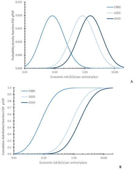
Figure 7.
Distribution of the economic risk (€/a) per animal place by the reduction of the gross margin for t = 1980, t = 2020 and t = 2030 shown by probability density functions (PDFs panel (A)) and cumulative distribution functions (CDFs panel (B)).
4. Discussion
Farmers require information on the likelihood and severity of future climate extremes, and their effects on farm animals, to make well-founded management decisions. The analysis presented here shows an increase of the frequency of four HS indices over the last four decades (Figure 4 and [11]). A significant time trend of the HS indices between 1981 and 2017 was determined. The poor variance estimate for the trends determined by a regression analysis resulted in a poor estimate of the test statistics for the SNR, which resulted in an incorrect inference about the trend [44]. Therefore, the nonparametric Mann-Kendall test was applied as well. Della-Marta, Haylock, Luterbacher and Wanner [35] used a piecewise detrending method for a much longer time series (since 1880), which was not useful for a time series of 37 years. A detailed review of appropriate distribution functions and methods to analyze the time trend can be found in Visser and Petersen [45]. Since we used a 20-year and a 10-year return period, the selected PDFs and the corresponding shapes of the right tails were not as sensitive as for longer return periods [45,46]. The goodness of the fit of the empirical data from the detrended and logarithmically transformed HS indices ΔEXT with a Gaussian distribution was demonstrated by the low values of the AIC and graphically shown in Figure 3. Especially the right tail was fitted well by the selected normal distribution.
The Expert Team on Climate Change Detection and Indices (ETCCDI) defined a set of so-called climate indices that describe different fields of climatic change [47]. Such climate indices are the mean number of summer days (maximum temperature above 25 °C), heat days (maximum temperature above 30 °C) or tropical nights (minimum temperature above 20 °C) per year. They are strongly connected to the indoor climate of confined livestock buildings. Klein, Tank and Können [48] investigated meteorological stations in Central Europe and found that the number of summer days increased by about two to four days per decade in the time period from 1946 to 1999. Compared to this, the mean number of summer days per year in the case study region of Wels was 42.3 in the period 1971–2000. The number increased by about six days on average to 48.8 in the period 1981–2010. Depending on different possible future climate change signals, this number could increase to values from 53.5 up to 62.7 until the middle of this century in the period 2036–2065. Heat days occur less frequently in this area. In the period 1971–2000, a mean number of 5.1 heat days per year was observed, whereas in the period 1981–2010 this number increased to 7.9 days on average. Tropical nights have a big influence on the health of the human population, especially in the case of several of such days in a row [49]. This effect can be expected for farm animals to an even greater extent. Sillmann and Roeckner [50] expected that tropical nights will increase in Central Europe by about 10–25 days on average between today and the end of the 21st century.
The simulation of the indoor climate was performed for a typical livestock building in Central Europe where the majority of pigs and poultry are kept [51]. Such systems are predominantly located in the Cfb temperate climate zone (Köppen-Geiger climate classification, temperate oceanic climate (warm temperature, fully humid, warm summers)). This conjunction between temperate climate and the density of confined livestock buildings [51,52] can be found not only in Central Europe but also in parts of North America and Asia (predominantly China).
HS indices can be calculated by weather-related parameters from a meteorological station by measured data, or by simulated data of indoor parameters [11,53,54]. The investigated relationship between HS indices, which are calculated by the indoor parameters and those calculated by meteorological parameters, showed a coefficient of determination above 80% and a slope of the linear regression between 1.17 and 2.13 (Figure 2, Table 2), which means that the indoor parameters were more sensitive to HS [25]. Nevertheless, the weather-related HS indices can be used as a reliable proxy for the indoor indices. However, the indoor simulation described the thermal environment of animals inside a confined livestock building in a more precise way. Its disadvantages are the resource demand to determine the system parameters of the building (for example the U value of the construction elements), the ventilation system (maximum and minimum ventilation rate, and key parameters of the control unit), and the livestock as a source of sensible and latent energy. Weather-related HS indices have the advantage of easily accessible input parameters provided by meteorological stations. In Austria, for example, about 270 stations with a mean distance of about 11 km provide data in a temporal resolution of one hour. This means that a representative meteorological station can be expected in the vicinity of a livestock building. The HS indices, calculated from meteorological data, could be published on a day-to-day basis, similar to other agrometeorological services, such as the growing degree days for plants [55,56,57].
Several adaptation measures are in use to alleviate heat stress and to improve the thermal environment of the animals kept inside livestock buildings [25,29]. Most of these measures require investments and increase running costs. To strengthen the economic resilience of livestock farms, and to allow for deliberate investment decisions, the economic risks should be estimated and managed. This article quantified the likelihood of HS for farm animals in 1980, 2020 and in 2030 (Figure 4). Subsequently, the economic risk was assessed by the product of the HS likelihood and the economic impact (Figure 7). The latter is expressed as losses in gross margins for growing-fattening pigs as a function of the ATHI75 heat stress index. The predictor of the cost function in St-Pierre, Cobanov and Schnitkey [36] was the HS index calculated by the THI and the threshold of XTHI = 75. The variability of this HS index was caused by differences in local climates across the entire USA (spatial variability), whereas the variability of the HS indices presented here was caused by the trend due to global warming. The assessment of the economic impact following the approach of St-Pierre, Cobanov and Schnitkey [36] included the reduction of the animals’ live mass at the end of the fattening period, the related reduction of feed required and the increased mortality of the animals. These traits were parameterized by linear functions. It is however not plausible that the impact of HS will be the same for the temperature range of 25 °C to 28 °C and for 30 °C to 33 °C. This fact was investigated by several authors [15,58,59]. In a European study about risk factors for mortality in fattening pigs, a significant seasonal impact with higher mortalities of pigs placed at the end of the year was found, which was associated with infectious diseases [60]. This finding was in contrast to a higher mortality in summer in the Midwest in the USA [23], which might be associated with a higher frequency of HS in this region. To the authors’ knowledge, no evaluation of mortality in fatteners during extreme weather periods has been performed so far. For this reason, the economic assessment of the impact of heat stress was mainly based on the decrease in livestock growth parameters. Other variable costs such as the market driven costs for piglets, veterinary services, energy for the ventilation system, and water consumption were not taken into account in this study, despite the effect of HS on these [11].
The economic risk for fattening pigs due to HS was quantified by the reduction of the gross margin for one animal place. For the period from 1980 to 2020 the mean reduction of the gross margin grew from 0.08 € a−1 to 1.57 € a−1 per animal place. Taking into account the likelihood of the occurrence of heat stress, the economic risk was determined for a repeat period of 20 years with 0.38 € a−1 for 1980 and 7.18 € a−1 per animal place for 2030. These additional costs due to HS can be compared to the cost of a misting system to reduce HS. Bridges, et al. [61] simulated the costs for Kentucky for 1983 (warm year) at 10.2 $ a−1 per animal place and 1995 (close to normal) at 1.5 $ a−1 per animal place, which lie in the same range.
This reduction of the gross margin due to HS has to be compared with the gross margin expected for a typical farm. The gross margin (without the building costs) depends on the level of animal performance in a range between 33 € a−1 and 42 € a−1 per animal place [62] for Germany and about 50 to 70 € a−1 per animal place for Austria (Federal Institute of Agricultural Economics AWI www.awi.bmnt.gv.at). For the US, Jacobson, et al. [63] estimated a gross margin of about 98 $ a−1 per animal place (without building costs).
Another consequence of increased HS results from its impact on livestock wellbeing, which can influence consumers’ willingness to pay for pork. Similarly, pork quality may decline. For example, an alteration of carcass composition and an increase in the risk of occurrence of pale, soft, exudative (PSE) meat in pigs can be expected [64,65] and may reduce revenue. In pigs, decreased carcass quality as a consequence of heat stress is reflected by pork processing problems due to a flimsier adipose tissue, increased lipid and decreased protein content [36,66]. Above the pig’s thermal neutral zone, nutrient energy sources are shifted from synthesis of products to maintenance of body homeostasis by heat release. On the other hand, heat stress can lead to a higher efficiency in conversion of dietary energy into body mass. Carcass tissue gain might be improved, while carcass composition and quality may be impaired [17,66]. In fattening pigs, an interaction of housing at 32 °C and limited space (0.66 m2 per pig) was found to be connected with an increased adipose iodine value and a decreased saturated:unsaturated fatty acids ratio. Pigs kept at higher temperature showed changes in carcass lipid and bacon quality, e.g., lean:fat ratio of bacon slices and increased quantity of collagen in belly fat [67].
Acute or chronic heat stress prior to slaughter can alter the chemical properties of pork by pH lower or higher than 5.6–5.7 within 3–5 h after slaughter. Under situations of increased temperature and metabolism prior to and during slaughter, lactic acid cell levels increase resulting in low pH, which damages muscle proteins followed by a high dripping loss (poor water-holding capacity), color and flavorless after cooking (pale, soft and exudative PSE). In the case of long-term stressors, no glycogen is available to be converted into lactic acid postmortem, resulting in a high pH value and dry meat, which can spoil rapidly (dark, firm and dry DFD). In general, heat stress was found to reduce food safety due to increased bacterial growth and shedding [65]. This means that the economic impact function based on the assumptions of St-Pierre, Cobanov and Schnitkey [36] likely underestimates the total costs for farmers caused by HS. An analysis of greenhouse gas and air pollutant emissions from pig production systems driven by climate change, which was based on the same data and indoor climate models, showed that emissions increased with climate change for the entire production chain from breeding to finishing [68,69]. Hence, the (externalized) climate and environmental-related costs for society will also increase. In the case of an internalization of external costs (e.g., with a tax on emissions) due to climate change, economic losses of pig production systems could further increase. Its effect depends on the competitiveness of markets, i.e., whether consumers take a share as well. Consequently, both the private and social costs from livestock production likely will increase with climate change.
Hansen, et al. [70] pointed out that insurance, conservation soil management, genetically adapted feed crops and diversified farming systems are the most important factors increasing resilience against climate change. The development of insurance in the livestock sector is generally lower than in the crop sector. Only a few insurance products for livestock are offered, predominantly for animals kept on pasture in developing countries and for sanitary assistance programs for severe diseases. Livestock risk management relies predominantly on sanitary assistance programs for major crises (diseases with high externalities), which are often subsidized by the public [71]. Weather index-based insurance is a relatively new tool that is helpful for farmers in managing risks. It pays out, based on an index such as the HS index, calculated by meteorological data from a local weather station, rather than based on a consequence of weather, such as a reduction of the average daily gain or the mortality of the livestock. Most of the weather index-based insurances are configured to the grassland keeping of animals and the impact of the availability of feed, mostly for extensive livestock production in India [72], Iran [73,74], Ethiopia [75,76], South Africa [77] and for tropical areas [78].
Since livestock production shows a high vulnerability caused by a relative scarcity of equity capital, risk transfer by means of weather derivatives or insurance could be attractive for farmers. Even the European Union [79] and COP21 leaders in 2015 [73] asked for risk management to assist farmers in addressing the most common risks, setting up mutual funds, and the compensation paid by such funds to farmers for losses suffered as a result of adverse climatic events. It is not only profitable efficiency, but also stability and liquidity of farms, which may be negatively influenced by HS, and insurance may help to alleviate these effects.
For weather index-based insurance as one option for farm risk management, the relevant indices have to be calculated from meteorological data to achieve an objective measure. Following the methodology for HS indices presented in this article, administrative costs and moral hazards can be minimized and allow companies to offer simple, affordable and transparent risk transfer [72]. Such indices describing drought, flooding or the occurrence of diseases, are highly correlated to local yields [55,80].
For intensive livestock production in confined houses, the economic risk by HS can be reflected in considerable monetary losses. Risk transfer mechanisms against HS-related economic losses will very often compete with adaptation measures in confined livestock buildings such as energy-saving air treatment systems, which cool the inlet air (e.g., cooling pads, earth-air-heat exchanger), use of certain building elements (e.g., insulation), optimizing building characteristics (e.g., spatial orientation), modification of the indoor climate at the animal level (e.g., fogging, cooling the drinking water, increasing air velocity), and adaptation of livestock management (e.g., reduction of stocking density) [29,81]. The use of such adaptation measures could be supported through discounted premiums [82].
5. Conclusions
The assessment of the economic risk due to global warming and the related HS on livestock kept inside confined buildings suggested a multistage process. (1) The temporal trend of meteorological parameters describing the environment of the livestock building was analyzed. It was shown that routinely measured air temperature and humidity data can be applied to assess the chosen HS indices. This approach is more feasible and straightforward than the determination of indoor parameters. The measured meteorological parameters drive the indoor climate of such buildings. (2) The likelihood of HS was estimated. Climate change leads to an unfavorable increasing trend of chosen weather-related HS indices. Beside an estimator of the expected value of an HS index, the uncertainty was assessed as well. This was demonstrated especially when investigating the consequence of global warming on the extreme values of the HS indices. The most relevant right tail of the detrended HS indices was fitted well by a normal distribution (Figure 3). Likelihood and exceedance probability for the occurrence of a certain weather-related HS index increased considerably during the last 40 years and will continue to increase in the near future (Figure 4 and Figure 5). Correspondingly, the return period for extreme values decreased from 10 years in 1980 to one year in 2020 (Table 7) and this trend is predicted to continue. (3) The impact of increased HS on the animals will cause a reduction of their performance. This depression was quantified as loss of gross margins. To quantify the economic impact of increasing HS, three parameters, namely, reduction of body mass at the end of the fattening period, dry matter intake and the increase of the mortality, were taken into account. (4) In the last step, the HS events assuming a probability of a return period of 10 years resulted in a growth of the economic risk from 0.27 € a−1 to 5.13 € a−1 per animal place, which is around 5% to 10% of gross margins for a typical farm. For farmers, such a risk assessment is an essential tool for management decisions like the implementation of adaption measures to reduce HS, thermal-tolerant and adapted breeds or feeding strategies by adjusting diet composition.
On a national level, the extreme hot year 2003 caused additional costs of 100 million € for the intensive livestock sector in France and the same amount in Spain. The fodder deficit lay in the range of 30% for Germany, Austria and Spain, about 40% in Italy and about 60% in France. In France, about 4 million broilers died. In Spain the mortality for broilers was in the range of 15 and 20% with an decrease of productivity by 25–30% [2].
The insurance sector is likely to become more relevant for future adaptation decisions, mostly based on weather index-based schemes, weather derivatives or catastrophe bonds [82]. Weather index-based insurance is a relatively new but innovative approach to insurance provision that pays out benefits based on a predetermined index for loss of assets and investments (reduction of animal performance, mortality etc.). Because index-based insurance does not necessarily require traditional services of insurance claim assessors, it allows a quicker and more objective process of claims settlement [72].
Author Contributions
Conceptualization, G.S., M.S., and W.Z.; methodology, G.S., W.Z., and M.S.; writing—original draft preparation, G.S.; writing—review and editing, M.S., W.Z., S.J.H., L.K., C.M., J.B., W.K., I.A., K.A., I.H.-P., and M.P. All authors have read and agreed to the published version of the manuscript.
Funding
The project PiPoCooL Climate change and future pig and poultry production: implications for animal health, welfare, performance, environment and economic consequences was funded by the Austrian Climate and Energy Fund in framework of the Austrian Climate Research Program (ACRP8–PiPoCooL–KR15AC8K12646).
Institutional Review Board Statement
Not applicable.
Informed Consent Statement
Not applicable.
Data Availability Statement
Data sharing not applicable.
Acknowledgments
Open Access Funding by the University of Veterinary Medicine Vienna.
Conflicts of Interest
The authors declare no conflict of interest.
References
- Murray-Tortarolo, G.N.; Jaramillo, V.J. The impact of extreme weather events on livestock populations: The case of the 2011 drought in Mexico. Clim. Chang. 2019. [Google Scholar] [CrossRef]
- COPA-COGECA. Assessment of the Impact of the Heat Wave and Drought of the Summer 2003 on Agricultural and Forestry; Comitêdês Organisations Professionalles de la Agricoles de la Communité Européenne/Comitê General de la Cooperation Agricole: Köln, Germany, 2004. [Google Scholar]
- Nardone, A.; Ronchi, B.; Lacetera, N.; Ranieri, M.S.; Bernabucci, U. Effects of climate changes on animal production and sustainability of livestock systems. Livest. Sci. 2010, 130, 57–69. [Google Scholar] [CrossRef]
- Özkan, Ş.; Vitali, A.; Lacetera, N.; Amon, B.; Bannink, A.; Bartley, D.J.; Blanco-Penedo, I.; De Haas, Y.; Dufrasne, I.; Elliott, J.; et al. Challenges and priorities for modelling livestock health and pathogens in the context of climate change. Environ. Res. 2016, 151, 130–144. [Google Scholar] [CrossRef] [PubMed]
- Bett, B.; Kiunga, P.; Gachohi, J.; Sindato, C.; Mbotha, D.; Robinson, T.; Lindahl, J.; Grace, D. Effects of climate change on the occurrence and distribution of livestock diseases. Prev. Vet. Med. 2017, 137, 119–129. [Google Scholar] [CrossRef]
- Morgan, E.R.; Wall, R. Climate change and parasitic disease: Farmer mitigation? Trends Parasitol. 2009, 25, 308–313. [Google Scholar] [CrossRef]
- Wall, R.; Rose, H.; Ellse, L.; Morgan, E. Livestock ectoparasites: Integrated management in a changing climate. Vet. Parasitol. 2011, 180, 82–89. [Google Scholar] [CrossRef]
- Van Dijk, J.; Sargison, N.D.; Kenyon, F.; Skuce, P.J. Climate change and infectious disease: Helminthological challenges to farmed ruminants in temperate regions. Animal 2010, 4, 377–392. [Google Scholar] [CrossRef]
- Skuce, P.J.; Morgan, E.R.; Van Dijk, J.; Mitchell, M. Animal health aspects of adaptation to climate change: Beating the heat and parasites in a warming Europe. Animal 2013, 7 (Suppl. 2), 333–345. [Google Scholar] [CrossRef]
- Hatfield, J.L.; Antle, J.; Garrett, K.A.; Izaurralde, R.C.; Mader, T.; Marshall, E.; Nearing, M.; Philip Robertson, G.; Ziska, L. Indicators of climate change in agricultural systems. Clim. Chang. 2018, 1–14. [Google Scholar] [CrossRef]
- Mikovits, C.; Zollitsch, W.; Hörtenhuber, S.J.; Baumgartner, J.; Niebuhr, K.; Piringer, M.; Anders, I.; Andre, K.; Hennig-Pauka, I.; Schönhart, M.; et al. Impacts of global warming on confined livestock systems for growing-fattening pigs: Simulation of heat stress for 1981 to 2017 in Central Europe. Int. J. Biometeorol. 2019, 63, 221–230. [Google Scholar] [CrossRef]
- Godde, C.M.; Mason-D’Croz, D.; Mayberry, D.E.; Thornton, P.K.; Herrero, M. Impacts of climate change on the livestock food supply chain; a review of the evidence. Glob. Food Secur. 2021, 28. [Google Scholar] [CrossRef]
- Bjerg, B.; Brandt, P.; Pedersen, P.; Zhang, G. Sows’ responses to increased heat load–A review. J. Therm. Biol. 2020, 94. [Google Scholar] [CrossRef] [PubMed]
- Hansen, R.K.; Bjerg, B. Optimal ambient Temperature with regard to Feed Efficiency and Daily Gain of finisher pigs. In Proceedings of the EurAgEng 2018 Conference, Wageningen, The Netherlands, 8–12 July 2018; pp. 8–12. [Google Scholar]
- Renaudeau, D.; Collin, A.; Yahav, S.; De Basilio, V.; Gourdine, J.L.; Collier, R.J. Adaptation to hot climate and strategies to alleviate heat stress in livestock production. Animal 2012, 6, 707–728. [Google Scholar] [CrossRef] [PubMed]
- Quiniou, N.; Dubois, S.; Noblet, J. Voluntary feed intake and feeding behaviour of group-housed growing pigs are affected by ambient temperature and body weight. Livest. Prod. Sci. 2000, 63, 245–253. [Google Scholar] [CrossRef]
- Johnson, J.S. Heat stress: Impact on livestock well-being and productivity and mitigation strategies to alleviate the negative effects. Anim. Prod. Sci. 2018, 58, 1404–1413. [Google Scholar] [CrossRef]
- Lacetera, N. Impact of climate change on animal health and welfare. Anim. Front. 2019, 1, 26–31. [Google Scholar] [CrossRef]
- Geers, R.; Berckmans, D.; Goedseels, V.; Wijnhoven, J.; Maes, F. A case-study of fattening pigs in Belgian contract farming. Mortality, efficiency of food utilization and carcass value of growing pigs, in relation to environmental engineering and control. Anim. Prod. 1984, 38, 105–111. [Google Scholar] [CrossRef]
- D’Allaire, S.; Drolet, R.; Brodeur, D. Sow mortality associated with high ambient temperatures. Can. Vet. J. 1996, 37, 237–239. [Google Scholar]
- Stalder, K.J. 2014 U.S. Pork Industry Productivity Analysis; National Pork Board: Des Moines, IA, USA, 2014.
- Agostini, P.; Fahey, A.; Manzanilla, E.; O’Doherty, J.; De Blas, C.; Gasa, J. Management factors affecting mortality, feed intake and feed conversion ratio of grow-finishing pigs. Animal 2014, 8, 1312–1318. [Google Scholar] [CrossRef]
- Maes, D.; Larriestra, A.; Deen, J.; Morrison, R. A retrospective study of mortality in grow-finish pigs in a multi-site production system. J. Swine Health Prod. 2001, 9, 267–273. [Google Scholar]
- King, D.; Schrag, D.; Dadi, Z.; Ye, Q.; Ghosh, A. Climate Change: A Risk Assessment; Centre for Science and Policy (CSaP) at the University of Cambridge: Cambridge, UK, 2017. [Google Scholar]
- Schauberger, G.; Mikovits, C.; Zollitsch, W.; Hörtenhuber, S.J.; Baumgartner, J.; Niebuhr, K.; Piringer, M.; Knauder, W.; Anders, I.; Andre, K.; et al. Global warming impact in confined livestock buildings: Efficacy of adaptation measures to reduce heat stress for growing-fattening pigs. Clim. Chang. 2019, 156, 567–587. [Google Scholar] [CrossRef]
- Godyń, D.; Herbut, P.; Angrecka, S.; Corrêa Vieira, F.M. Use of different cooling methods in pig facilities to alleviate the effects of heat stress-a review. Animals 2020, 10, 1459. [Google Scholar] [CrossRef] [PubMed]
- Gauly, M.; Ammer, S. Review: Challenges for dairy cow production systems arising from climate changes. Animal 2020, 14, S196–S203. [Google Scholar] [CrossRef] [PubMed]
- Bjerg, B.; Brandt, P.; Sørensen, K.; Pedersen, P.; Zhang, G. Review of methods to mitigate heat stress among sows. In Proceedings of the 2019 ASABE Annual International Meeting, Boston, MT, USA, 7–10 July 2019; pp. 1–10. [Google Scholar]
- Schauberger, G.; Hennig-Pauka, I.; Zollitsch, W.; Hörtenhuber, S.J.; Baumgartner, J.; Niebuhr, K.; Piringer, M.; Knauder, W.; Anders, I.; Andre, K.; et al. Efficacy of adaptation measures to alleviate heat stress in confined livestock buildings in temperate climate zones. Biosyst. Eng. 2020, 200, 157–175. [Google Scholar] [CrossRef]
- Beniston, M.; Stoffel, M.; Guillet, S. Comparing observed and hypothetical climates as a means of communicating to the public and policymakers: The case of European heatwaves. Environ. Sci. Policy 2017, 67, 27–34. [Google Scholar] [CrossRef]
- Orth, R.; Zscheischler, J.; Seneviratne, S.I. Record dry summer in 2015 challenges precipitation projections in Central Europe. Nature. Sci. Rep. 2016, 6, 28334. [Google Scholar] [CrossRef]
- Anders, I.; Stagl, J.; Auer, I.; Pavlik, D. Climate Change in Central and Eastern Europe. In Managing Protected Areas in Central and Eastern Europe under Climate Change; Rannow, S., Neubert, M., Eds.; Advances in Global Change Research No 58; Springer: Dordrecht, The Netherlands; Heidelberg, Germany; New York, NY, USA; London, UK, 2014. [Google Scholar]
- Beniston, M.; Stephenson, D.B.; Christensen, O.B.; Ferro, C.A.; Frei, C.; Goyette, S.; Halsnaes, K.; Holt, T.; Jylhä, K.; Koffi, B. Future extreme events in European climate: An exploration of regional climate model projections. Clim. Chang. 2007, 81, 71–95. [Google Scholar] [CrossRef]
- Della-Marta, P.; Beniston, M. Summer heat waves in Western Europe, their past change and future projections. In Climate Variability and Extremes during the Past 100 Years; Springer: Berlin/Heidelberg, Germany, 2008; pp. 235–250. [Google Scholar]
- Della-Marta, P.M.; Haylock, M.R.; Luterbacher, J.; Wanner, H. Doubled length of western European summer heat waves since 1880. J. Geophys. Res. Atmos. 2007, 112. [Google Scholar] [CrossRef]
- St-Pierre, N.R.; Cobanov, B.; Schnitkey, G. Economic losses from heat stress by US livestock industries. J. Dairy Sci. 2003, 86, E52–E77. [Google Scholar] [CrossRef]
- Toeglhofer, C.; Mestel, R.; Prettenthaler, F. Weather Value at Risk: On the measurement of noncatastrophic weather risk. Weather Clim. Soc. 2012, 4, 190–199. [Google Scholar] [CrossRef]
- Kottek, M.; Grieser, J.; Beck, C.; Rudolf, B.; Rubel, F. World map of the Köppen-Geiger climate classification updated. Meteorol. Z. 2006, 15, 259–263. [Google Scholar] [CrossRef]
- Schauberger, G.; Piringer, M.; Petz, E. Steady-state balance model to calculate the indoor climate of livestock buildings, demonstrated for fattening pigs. Int. J. Biometeorol. 2000, 43, 154–162. [Google Scholar] [CrossRef] [PubMed]
- Schauberger, G.; Piringer, M.; Petz, E. Diurnal and annual variation of odour emission from animal houses: A model calculation for fattening pigs. J. Agric. Eng. Res. 1999, 74, 251–259. [Google Scholar] [CrossRef]
- International Commission of Agricultural Engineering. 2nd Report of Working Group on Climatization of Animal Houses; Centre for Climatization of Animal Houses-Advisory Services, Faculty of Agricultural Sciences, State University of Ghent: Ghent, Belgium, 1992; p. 119. [Google Scholar]
- Vitt, R.; Weber, L.; Zollitsch, W.; Hörtenhuber, S.J.; Baumgartner, J.; Niebuhr, K.; Piringer, M.; Anders, I.; Andre, K.; Hennig-Pauka, I.; et al. Modelled performance of energy saving air treatment devices to mitigate heat stress for confined livestock buildings in Central Europe. Biosyst. Eng. 2017, 164, 85–97. [Google Scholar] [CrossRef]
- Schönwiese, C.-D. Praktische Statistik für Meteorologen und Geowissenschaftler; Gebrüder Borntraeger: Berlin/Stuttgart, Germany, 2013. [Google Scholar]
- Nunifu, T.K.; Fu, L. Methods and Procedures for Trend Analysis of Air Quality Data; Ministry of Environment and Parks: Edmonton, AB, Canada, 2019.
- Visser, H.; Petersen, A. Inferences on weather extremes and weather-related disasters: A review of statistical methods. Clim. Past 2012, 8, 265–286. [Google Scholar] [CrossRef]
- Wigley, T.M.L. The effect of changing climate on the frequency of absolute extreme events. Clim. Chang. 2009, 97, 67. [Google Scholar] [CrossRef]
- Klein Tank, A.; Zwiers, F.; Zhang, X. Guidelines on Analysis of Extremes in a Changing Climate in Support of Informed Decisions for Adaptation (WCDMP-72); World Meteorological Organization: Geneva, Switzerland, 2009. [Google Scholar]
- Klein Tank, A.M.G.; Können, G.P. Trends in indices of daily temperature and precipitation extremes in Europe, 1946–1999. J. Clim. 2003, 16, 3665–3680. [Google Scholar] [CrossRef]
- Fischer, E.M.; Schär, C. Consistent geographical patterns of changes in high-impact European heatwaves. Nat. Geosci. 2010, 3, 398–403. [Google Scholar] [CrossRef]
- Sillmann, J.; Roeckner, E. Indices for extreme events in projections of anthropogenic climate change. Clim. Chang. 2008, 86, 83–104. [Google Scholar] [CrossRef]
- Robinson, T.; Thornton, P.; Franceschini, G.; Kruska, R.; Chiozza, F.; Notenbaert, A.; Cecchi, G.; Herrero, M.; Epprecht, M.; Fritz, S. Global Livestock Production Systems; Food and Agriculture Organization of the United Nations (FAO): Rome, Italy, 2011. [Google Scholar]
- Robinson, T.P.; Wint, G.R.W.; Conchedda, G.; Van Boeckel, T.P.; Ercoli, V.; Palamara, E.; Cinardi, G.; D’Aietti, L.; Hay, S.I.; Gilbert, M. Mapping the global distribution of livestock. PLoS ONE 2014, 9, e96084. [Google Scholar] [CrossRef]
- Turnpenny, J.R.; Parsons, D.J.; Armstrong, A.C.; Clark, J.A.; Cooper, K.; Matthews, A.M. Integrated models of livestock systems for climate change studies. 2. Intensive systems. Glob. Chang. Biol. 2001, 7, 163–170. [Google Scholar] [CrossRef]
- Panagakis, P.; Axaopoulos, P. Comparison of two modeling methods for the prediction of degree-hours and heat-stress likelihood in a swine building. Trans. Asae 2004, 47, 585–590. [Google Scholar] [CrossRef]
- Prokopy, L.S.; Haigh, T.; Mase, A.S.; Angel, J.; Hart, C.; Knutson, C.; Lemos, M.C.; Lo, Y.-J.; McGuire, J.; Morton, L.W. Agricultural advisors: A receptive audience for weather and climate information? Weather Clim. Soc. 2013, 5, 162–167. [Google Scholar] [CrossRef]
- Weiss, A.; Crowder, L.; Bernardi, M. Communicating agrometeorological information to farming communities. Agricult. For. Meteorol. 2000, 103, 185–196. [Google Scholar] [CrossRef]
- WMO. Guide to Agricultural Meteorological Practices (GAMP); World Meteorological Organization: Geneva, Switzerland, 2010. [Google Scholar]
- Renaudeau, D.; Gourdine, J.L.; St-Pierre, N.R. A meta-analysis of the effects of high ambient temperature on growth performance of growing-finishing pigs. J. Anim. Sci. 2011, 89, 2220–2230. [Google Scholar] [CrossRef]
- Stalder, K.J. 2016 U.S. Pork Industry Productivity Analysis; National Pork Board: Des Moines, IA, USA, 2016.
- Maes, D.; Duchateau, L.; Larriestra, A.; Deen, J.; Morrison, R.; Kruif, A.d. Risk factors for mortality in grow-finishing pigs in Belgium. Zoonoses Public Health 2004, 51, 321–326. [Google Scholar] [CrossRef]
- Bridges, T.; Turner, L.; Gates, R. Economic evaluation of misting-cooling systems for growing/finishing swine through modeling. Appl. Eng. Agric. 1998, 14, 425–430. [Google Scholar] [CrossRef]
- KTBL. Faustzahlen für die Landwirtschaft, 15 ed.; Kuratorium für Technik und Bauwesen in der Landwirtschaft, KTBL: Darmstadt, Germany, 2018; p. 1384. [Google Scholar]
- Jacobson, L.D.; Schmidt, D.R.; Lazarus, W.F.; Koehler, R. Reducing the Environmental Footprint of Pig Finishing Barns. In Proceedings of the 2011 SABE Annual International Meeting, Louisville, KY, USA, 7–10 August 2011. [Google Scholar]
- Zhang, M.; Dunshea, F.R.; Warner, R.D.; DiGiacomo, K.; Osei-Amponsah, R.; Chauhan, S.S. Impacts of heat stress on meat quality and strategies for amelioration: A review. Int. J. Biometeorol. 2020, 64, 1613–1628. [Google Scholar] [CrossRef]
- Gonzalez-Rivas, P.A.; Chauhan, S.S.; Ha, M.; Fegan, N.; Dunshea, F.R.; Warner, R.D. Effects of heat stress on animal physiology, metabolism, and meat quality: A review. Meat Sci. 2020, 162, 108025. [Google Scholar] [CrossRef]
- Ross, J.W.; Hale, B.J.; Gabler, N.K.; Rhoads, R.P.; Keating, A.F.; Baumgard, L.H. Physiological consequences of heat stress in pigs. Anim. Prod. Sci. 2015, 55, 1381–1390. [Google Scholar] [CrossRef]
- White, H.M.; Richert, B.T.; Schinckel, A.P.; Burgess, J.R.; Donkin, S.S.; Latour, M.A. Effects of temperature stress on growth performance and bacon quality in grow-finish pigs housed at two densities. J. Anim. Sci. 2008, 86, 1789–1798. [Google Scholar] [CrossRef] [PubMed]
- Hörtenhuber, S.J.; Schauberger, G.; Mikovits, C.; Schönhart, M.; Baumgartner, J.; Niebuhr, K.; Piringer, M.; Anders, I.; Andre, K.; Hennig-Pauka, I.; et al. The effect of climate change-induced temperature increase on performance and environmental impact of intensive pig production systems. Sustainability 2020, 12, 9442. [Google Scholar] [CrossRef]
- Schauberger, G.; Piringer, M.; Mikovits, C.; Zollitsch, W.; Hörtenhuber, S.J.; Baumgartner, J.; Niebuhr, K.; Anders, I.; Andre, K.; Hennig-Pauka, I.; et al. Impact of global warming on the odour and ammonia emissions of livestock buildings used for fattening pigs. Biosyst. Eng. 2018, 175, 106–114. [Google Scholar] [CrossRef]
- Hansen, J.; Hellin, J.; Rosenstock, T.; Fisher, E.; Cairns, J.; Stirling, C.; Lamanna, C.; van Etten, J.; Rose, A.; Campbell, B. Climate risk management and rural poverty reduction. Agric. Syst. 2019, 172, 28–46. [Google Scholar] [CrossRef]
- Bielza, M.; Stroblmair, J.; Gallego Pinilla, F.J.; Costanza, C.; Dittmann, C. Agricultural risk management in Europe. In Proceedings of the European Association of Agricultural Economists, 101st Seminar, Berlin, Germany, 5–6 July 2007. [Google Scholar]
- Warner, K.; Ranger, N.; Surminski, S.; Arnold, M.; Linnerooth-Bayer, J.; Michel-Kerjan, E.; Kovacs, P.; Herweijer, C. Adaptation to Climate Change: Linking Disaster Risk Reduction and Insurance; United Nations International Strategy for Disaster Reduction Secretariat (UNISDR): Geneva, Switzerland, 2009. [Google Scholar]
- Surminski, S.; Bouwer, L.M.; Linnerooth-Bayer, J. How insurance can support climate resilience. Nat. Clim. Chang. 2016, 6, 333–334. [Google Scholar] [CrossRef]
- Biglari, T.; Maleksaeidi, H.; Eskandari, F.; Jalali, M. Livestock insurance as a mechanism for household resilience of livestock herders to climate change: Evidence from Iran. Land Use Policy 2019, 87. [Google Scholar] [CrossRef]
- Gebrekidan, T.; Guo, Y.; Bi, S.; Wang, J.; Zhang, C.; Wang, J.; Lyu, K. Effect of index-based livestock insurance on herd offtake: Evidence from the Borena zone of southern Ethiopia. Clim. Risk Manag. 2018. [Google Scholar] [CrossRef]
- Amare, A.; Simane, B.; Nyangaga, J.; Defisa, A.; Hamza, D.; Gurmessa, B. Index-based livestock insurance to manage climate risks in Borena zone of southern Oromia, Ethiopia. Clim. Risk Manage. 2019, 25. [Google Scholar] [CrossRef]
- Oduniyi, O.S.; Antwi, M.A.; Tekana, S.S. Farmers’ willingness to pay for index-based livestock insurance in the North West of South Africa. Clim. 2020, 8, 47. [Google Scholar] [CrossRef]
- Chantarat, S.; Mude, A.G.; Barrett, C.B.; Turvey, C.G. The Performance of Index Based Livestock Insurance: Ex Ante Assessment in the Presence of a Poverty Trap. 2009. Available online: https://ssrn.com/abstract=1844751 (accessed on 2 February 2021).
- Regulation (EU) No 1305/2013 of the European Parliament and of the Council of 17 December 2013 on Support for Rural Development by the European Agricultural Fund for Rural Development (EAFRD) and Repealing Council Regulation (EC) No 1698/2005. Available online: https://eur-lex.europa.eu/legal-content/EN/TXT/PDF/?uri=CELEX:32013R1305&from=EN (accessed on 2 February 2021).
- Hazell, P.; Anderson, J.; Balzer, N.; Hastrup Clemmensen, A.; Hess, U.; Rispoli, F. The potential for Scale and Sustainability in Weather Index Insurance for Agriculture and Rural Livelihoods; World Food Programme (WFP): Rome, Italy, 2010. [Google Scholar]
- Prettenthaler, F.; Köberl, J.; Bird, D.N. ‘Weather Value at Risk’: A uniform approach to describe and compare sectoral income risks from climate change. Sci. Total Environ. 2016, 543, 1010–1018. [Google Scholar] [CrossRef]
- Chambwera, M.; Heal, G.; Dubeux, C.; Hallegatte, S.; Leclerc, L.; Markandya, A.; McCarl, B.A.; Mechler, R.; Neumann, J.E. Economics of adaptation. In Climate Change 2014: Impacts, Adaptation, and Vulnerability. Part A: Global and Sectoral Aspects. Contribution of Working Group II to the Fifth Assessment Report of the Intergovernmental Panel of Climate Change; Field, C.B., Barros, V.R., Dokken, D.J., Mach, K.J., Mastrandrea, M.D., Bilir, T.E., Chatterjee, M., Ebi, K.L., Estrada, Y.O., Genova, R.C., et al., Eds.; Cambridge University Press: Cambridge, UK; New York, NY, USA, 2014; pp. 945–977. [Google Scholar]
Publisher’s Note: MDPI stays neutral with regard to jurisdictional claims in published maps and institutional affiliations. |
© 2021 by the authors. Licensee MDPI, Basel, Switzerland. This article is an open access article distributed under the terms and conditions of the Creative Commons Attribution (CC BY) license (http://creativecommons.org/licenses/by/4.0/).