Article

Estimation of Reference Evapotranspiration during the Irrigation Season Using Nine Temperature-Based Methods in a Hot-Summer Mediterranean Climate

by
Gonçalo C. Rodrigues
1,2,* and
Ricardo P. Braga
2
1
LEAF—Linking Landscape, Environment, Agriculture and Food, Instituto Superior de Agronomia, Universidade de Lisboa, Tapada da Ajuda, 1349-017 Lisboa, Portugal
2
Instituto Superior de Agronomia, Universidade de Lisboa, Tapada da Ajuda, 1349-017 Lisboa, Portugal
*
Author to whom correspondence should be addressed.
Agriculture 2021, 11(2), 124; https://doi.org/10.3390/agriculture11020124
Submission received: 6 January 2021 / Revised: 30 January 2021 / Accepted: 1 February 2021 / Published: 4 February 2021

Abstract

:
The FAO-56 Penman–Monteith (PM) equation is regarded as the most accurate equation to estimate reference evapotranspiration (ETo). However, it requires a broad range of data that may not be available or of reasonable quality. In this study, nine temperature-based methods were assessed for ETo estimation during the irrigation at fourteen locations distributed through a hot-summer Mediterranean climate region of Alentejo, Southern Portugal. Additionally, for each location, the Hargreaves–Samani radiation adjustment coefficient (kRs) was calibrated and validated to evaluate the appropriateness of using the standard value, creating a locally adjusted Hargreaves–Samani (HS) equation. The accuracy of each method was evaluated by statistically comparing their results with those obtained by PM. Results show that the calibration of the kRs, a locally adjusted HS method can be used to estimate daily ETo acceptably well, with RMSE lower than 0.88 mm day−1, an estimation error lower than 4% and a R2 higher than 0.69, proving to be the most accurate model for 8 (out of 14) locations. A modified Hargreaves–Samani method also performed acceptably for 4 locations, with a RMSE of 0.72–0.84 mm day−1, a slope varying from 0.95 to 1.01 and a R2 higher than 0.78. One can conclude that, when weather data is missing, a calibrated HS equation is adequate to estimate ETo during the irrigation season.

1. Introduction

A simple method to estimate crop water requirements is through the computation of reference evapotranspiration (ETo). If accurate, these computations serve as a basis for several assessments such as water management, irrigation system design and management, irrigation scheduling, and crop modeling [1,2,3,4,5,6,7,8,9]. There are several methods for estimating ETo, being the FAO-56 application of the Penman–Monteith (PM) equation [4] widely regarded as the most accurate. The method provides consistent ETo values in many regions and climates [10,11] and it has long been accepted worldwide as a good ETo estimator when compared with other methods [12,13,14,15,16,17,18]. The PM equation presents certain advantages when compared with other ETo estimation methods. It can be used globally without the need for additional parameter estimations and it is well documented, has been implemented, and has been extensively validated. The major constraint of using the PM equation is the broad range of required data. Its physically based approach requires measurements of air temperature, windspeed, relative humidity, and solar radiation [4]. The number of stations where all this data is recorded is limited; an additional issue that could be brought into discussion is the data quality. One could also argue about the quality of the observed parameters.
The limitation of available and reliable data motivated Hargreaves and Samani [19] to develop a simpler method—known as the Hargreaves–Samani method (HS)—where only data of maximum and minimum air temperature, extraterrestrial radiation, and a radiation adjustment coefficient (kRs) are required. Since extraterrestrial radiation is an astronomical data and can easily be estimated for a certain day and location, only observed maximum and minimum air temperatures are required. Similar approaches were also developed such as Hargreaves–Samani [19], modified Hargreaves–Samani [20,21], Schendel [22], Baier-Robertson [23], and Trajkovic [24]. These methods are widely compared with PM by different authors [15,18,25,26,27,28,29]. Having pragmatic ETo estimation methods helps to improve water use efficiency. It can be used on simple weather prediction in order to promote a forward-looking irrigation scheduling.
Tabari and Talaee [26] used three Hargreaves-based equations to estimate ETo in Iran (with Köppen–Geiger climates BWh, BWk, BSk, Dsa, and Dsb) and compared the results with PM ETo estimations, leading to root mean square error (RMSE) varying from 0.49 to 1.60 mm day−1. A similar study in Jordan was performed by Mohawesh and Talozi [15] where the accuracy of the original Hargreaves–Samani (HS) and the modified Hargreaves–Samani (MHS) equations, as proposed by Droogers and Allen [21], were compared with PM in a Köppen–Geiger BWh BSh climates. Results showed a RMSE ranging from 0.614 to 1.303 mm day−1 for HS and varying from 0.557 to 2.033 mm day−1 for the ModHS methods.
Raziei and Pereira [26] compared both HS and PM for 40 weather stations located across Iran, covering different climatic zones, from humid to hyperarid. For humid zones, ETo estimation RMSE varied from 0.18 to 0.37 mm day−1, while for semiarid locations it varied from 0.27 to 0.81 mm day−1; for hyperarid zones the RMSE ranged from 0.64 to 0.97 mm day−1, showing that the estimation error tends to be higher with the increase of aridity. Paredes et al. [18] also assessed the accuracy of the Hargreaves–Samani method after calibrating the kRs factor for Azores, Portugal. ETo estimations using this method led to a RMSE varying for 0.47–0.86 mm day−1 and a coefficient of determination ranging from 0.57 to 0.79 based on a radiation adjustment coefficient that varied from 0.14 to 0.23 °C−0.5.
Two complementary studies were performed by Valipour and Eslamian [27] and by Valipour [29] where, for 31 locations from Iran, the accuracy to estimate ETo of various temperature-based methods were compared with PM, including the original HS, four MHS (including those proposed by [20,21]), Schendel (SCH), and Baier-Robertson (B&R) methods. Results showed that the MHS equations proved to be the most accurate for 27 (out of 31) locations with a coefficient of determination (R2) varying from 0.9762 to 0.9990 proving its effectiveness to estimate ETo when limited data is available.
Akhavan et al. [29] compared nine temperature-based methods with PM to estimate actual evapotranspiration of maize in Karaj, Iran—a Köppen–Geiger climates Csa, using two different crop coefficient approaches—single and dual. Both these methods differ since dual crop coefficient methodology consists on a separate computation of the two components of crop evapotranspiration, plant transpiration, which is represented by the basal crop coefficient, and soil evaporation, represented by the soil evaporation coefficient [4]. This study including the equation proposed by Baier and Robertson [23], Schendel [22], Droogers and Allen [20], Trajkovic [24], and Berti et al. [21]. Results showed that the RMSE varied from 1.97 to 5.80 mm day−1 and from 0.88 to 8.51 mm day−1 for single and dual crop coefficients approaches, respectively. For both scenarios a modified Hargreaves–Samani method performed the best while the Schendel method performed the worst.
These studies have shown that temperature-based methods can be as nearly as accurate as PM in estimating ETo, suggesting their use where reliable full dataset is lacking. However, and since each climatic condition contains a wide range of magnitude of each weather parameter (e.g., temperature, relative humidity, wind speed, solar radiation, etc.), the results of previous studies may not be applicable for other climates without further validation of each equation. Additionally, they only provide information when using each equation for the whole year, lacking the evaluation of each equation specifically during the irrigation season, when estimations of ETo are really required for irrigation scheduling and management.
The main objective of this study was to evaluate the performance of nine temperature-based methods to estimate PM reference evapotranspiration for 14 locations of Alentejo Region, Southern Portugal, a hot summer and Mediterranean climate region Csa, during the irrigation season (April to October). The specific objectives are: (1) to evaluate the estimation performance of temperature-based methods by comparison with the PM method during the irrigation season; (2) to calibrate and validate the Hargreaves model for each location to further improve its performance; (3) evaluate the necessity of location-by-location calibration vs. whole region calibration; and (4) to determine the best model based on the weather conditions of each location with the practical purpose of irrigation scheduling.

2. Materials and Methods
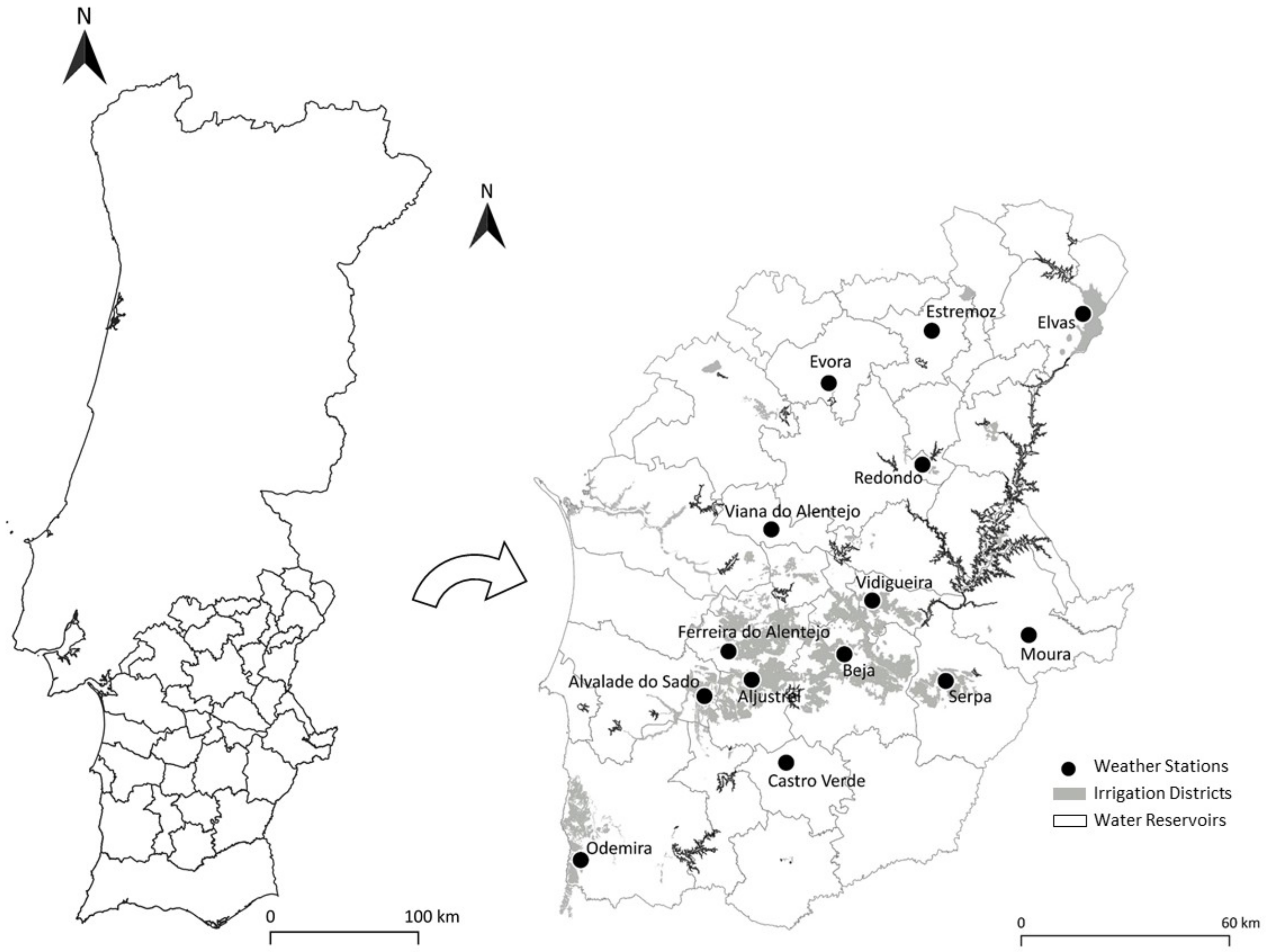
2.1. Study Area

This study was conducted in Alentejo Region, Southern Portugal, and used meteorological data from 14 locations across the region where the Irrigation Operation and Technology Center (COTR) has a network of full weather stations operating and collecting incoming maximum and minimum air temperature, relative humidity, wind speed, rainfall, and solar radiation. All data is daily validated by a team of experienced technicians, assuring its quality and feasibility.
Figure 1 and Table 1 respectively present the geographical position of the weather data locations, and their coordinates and period of observation. The region has a Csa climate according to Köppen–Geiger classification and is characterized by a semiarid Mediterranean climate of hot and dry season in the summer and mild temperature associated to annual rainfall in winter. Irrigation is crucial to achieve farming sustainability and profitability in the Alentejo region [8]. Additionally, and due to recurrent water scarcity, one way to achieve these goals is through the improvement of water use efficiency. Table 2 presents the yearly mean and standard deviation of main weather variables at each assessed location, including for the peak month of July.

2.2. Temperature-Based ETo Estimation Methods

All of the data collected were used to estimate the reference evapotranspiration using nine temperature-based models and were compared with PM equation to evaluate the accuracy of each method (Table 3). Those methods were selected based on its low data and demonstrated capacity to estimated ETo in other climates.
ETo is the reference crop evapotranspiration (mm day−1), Rn is the net radiation (MJ m−2 day−1), G is the soil heat flux (MJ m−2 day−1), γ is the psychrometric constant (kPa °C−1), es is the saturation vapor pressure (kPa), ea is the actual vapor pressure (kPa), Δ is the slope of the saturation vapor pressure-temperature curve (kPa °C−1), u2 is the mean daily wind speed at 2 m (m s−1), H is the elevation (m), ϕ is the latitude (rad), Tmax is the maximum air temperature (°C), Tmin is the minimum air temperature (°C), Tavg is the average air temperature (°C), RH is the average relative humidity (%), Ra is the extra-terrestrial radiation (MJ m−2 day−1), Rs is the solar radiation (MJ m−2 day−1), P is the monthly precipitation (mm), and kRs, n, and k are experimental coefficients.
For the Hargreaves–Samani equation, the empirical coefficient kRs was originally considered to range from 0.16 to 0.19 °C−0.5, respectively for “interior” or “coastal” regions [4]. In the original version of the Hargreaves–Samani (HS) equation [19], a bulk constant term of 0.023, known as the Hargreaves coefficient, is used. It corresponds to the product 0.0135 × kRs, with kRs = 0.17 °C−0.5, and 0.0135 representing a conversion of the units’ constant. However, kRs is supposed to vary with altitude, reflecting the changes of air pressure and volumetric heat capacity of the atmosphere [31]. Therefore, kRs should vary spatially, internalizing the effects of the site elevation and distance to sea [4]. For a similar climatic region, Moratiel et al. [32] evaluated the effectiveness of kRs calibration, both regionally and seasonally, and concluded that, when calibrating this factor, ETo estimations may improve, leading to a decrease of the RMSE from 0.62 to 0.54 mm day−1. Thus, one should argue that a constant kRs = 0.17 or the established range of 0.16–0.19 °C−0.5 for “interior” or “coastal” regions may not be suitable for all locations, requiring its calibration to reflect the site-specific conditions; however, when insufficient data is available, the original value may be used.
As for this study, two approaches were used for the Hargreaves–Samani equation. One where a standard kRs of 0.17 °C−0.5 was used for all locations as proposed by [19]. Another, where kRs was adjusted for each location. Adopting a trial and error procedure, being calibrated using 50% of the years, randomly chosen, from the dataset, and validated for the independent dataset obtained for the remainder of the years.
Along with the Hargreaves–Samani equation, five HS modified methods were also used—modified Hargreaves 1 (ModHS1), modified Hargreaves 2 (ModHS2), modified Hargreaves 3 (ModHS3), modified Hargreaves 4 (ModHS4), and Trajkovic (TR). These models vary from the original method since some parameters were modified, namely the kRs, the empirical temperature coefficient (HT) and the empirical Hargreaves exponent (HE). As stated, for the original HS, kRs = 0.17 °C−0.5, HT = 17.8, and HE = 0.5. For ModHS1, the bulk constant term of 0.023 was altered, resulting from the adoption of a kRs = 0.22 °C−0.5. Additionally, both HT and HE where adjusted, resulting on HT = 20 and HE = 0.4. Both ModHS2 and ModHS4 were also adjusted, with the former having a HT = 16.8 and the latter a HE = 0.517; as for radiation adjustment coefficient, a kRs = 0.19 and 0.14 °C−0.5 was used, respectively. For ModHS3 both HT and HE were also modified to 17 and 0.76, respectively, and a kRs = 0.10 °C−0.5 was used. This method includes rainfall as an added parameter to estimate ETo since, according to [20], the precipitation can in some regards represent relative levels of humidity, improving the method accuracy. As for TR, HE was adjusted, equaling 0.424.
Three other equations were also evaluated — Schendel (SCH), Baier and Robertson (B&R), and Enku and Melesse (E&M). B&R requires the same data as the original HS but it consists in a different approach (vd. Table 2). As for SCH an additional parameter is used—average relative humidity (RH)—and Ra is not considered to estimate ETo. E&M presents itself as the less data demanding method since it only requires the maximum and average temperature; the latter was used to locally adjust the experiment coefficient k.

2.3. Evaluation Criteria

The accuracy of each method was assessed by comparing their results with those of the PM equation through the indicators listed below:
(1)
The coefficients of regression and determination relating the PM and temperate-based ETo, b and R2 respectively, are defined as:
b   =   i   =   1 n ET PMi ET TBi i   =   1 n ET PMi 2
R 2   =   i   =   1 n ET PMi     ET PM ¯ ET TBi     ET TB ¯ i   =   1 n ET PMi     ET PM ¯ 2 0.5 i   =   1 n ET TBi   ET TB ¯ 2 0.5 2
(2)
The root mean square error, RMSE, which characterizes the variance of the estimation error:
RMSE = i = 1 n ET TBi     ET PMi 2 n 0.5
where ETPMi and ETTBi (i = 1, 2, …, n) represent pairs of values of ETo estimated using PM equation and other temperature-based method, respectively, for a given variable and ET PM ¯ and ET TB ¯ are the respective mean values and n is the number of days used in the assessment.

3. Results

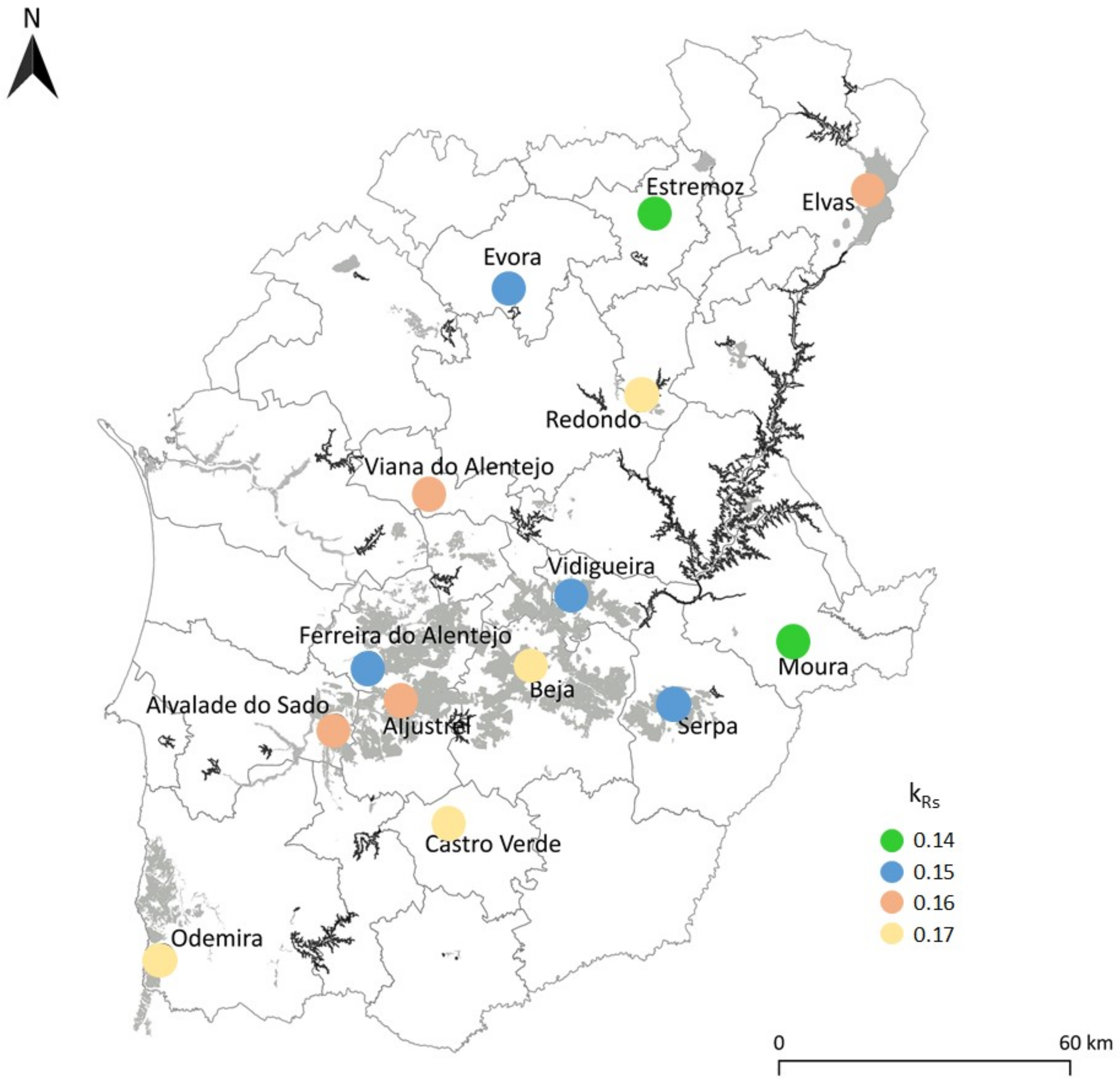
3.1. Calibration and Validation of Radiation Factor (kRs)

As previously stated, estimations of ETo may be performed using the Hargreaves–Samani equation with a locally calibrated and validated radiation adjustment coefficient kRs, thus resulting in an adjusted HS equation. Table 4 shows the calibrated and validated kRs values for each one of the 14 locations and for the entire Alentejo region. Table 4 also presents the statistical summary (b, R2, and RMSE) of ETo estimates for each location, that resulted from adopting the Adjusted HS equation, for calibration, validation and all years, and the ETo estimations that resulting from using the original HS equation.
Results (Table 4) show that the estimation accuracy of ETo when using the Hargreaves–Samani equation, after the calibration of kRs for each site, improved for 10 locations. When using the standard kRs, b varied from 0.96 to 1.23 (with only CV resulting in a b < 1.00), R2 values range from 0.69 to 0.83, and RMSE values varying from 0.65 to 1.38 mm day−1. When adopting the calibrated kRs for each location, these indicators improved significantly, with b ranging from 0.96 to 1.01 and a RMSE varying from 0.64 to 0.88 mm day−1, while the correlation (R2) remains the same as expected. Some locations stand out from the set: the RMSE for Moura decreased from 1.38 to 0.71 mm day−1 (with b decreasing from 1.23 to 1.01), while for Estremoz it decreased from 1.10 to 0.70 mm day−1 (with b decreasing from 1.16 to 0.96), representing a decrease of 19 and 36%, respectively. As for the Alentejo region, the calibration of kRs led to acceptable results with a slope of 1.0 and a RMSE equal to 0.86 mm day−1, both in line with the accuracy found for each individual location.
Figure 2 and Figure 3 try to show the effect of site-specific conditions over kRs. As discussed previously, and according to Allen [31] and Allen et al. [4], the kRs is supposed to reflect the volumetric heat capacity of the atmosphere, leading to lower kRs values with higher elevation and higher distance to the sea. Analyzing Figure 2 it can be concluded that “coastal” locations tended to show a higher kRs, while the “interior” site led to lower values; exception made for Beja (kRs = 0.17 °C−0.5), Castro Verde (kRs = 0.17 °C−0.5), Redondo (kRs = 0.17 °C−0.5), and Elvas (kRs = 0.16 °C−0.5) where lower values would be expected. One can assume that due to the presence of irrigation districts and water reservoirs close to each site the influence of air moisture on the volumetric heat capacity of the atmosphere can affect the radiation constant.

3.2. Estimating ETo by Temperature-Based Methods

The nine temperature-based methods were used to estimate daily ETo (mm day−1) for the 14 locations and were conducted from April to October, the period that covers the growing season of the main irrigated crops in Alentejo. The ETo values estimated by the all temperature-based equations were compared with estimates by the standard FAO-56 PM equation. The statistical summary (b, R2, and RMSE) of ETo estimates for the 14 locations are presented in Table 5.
The original Hargreaves–Samani (HS) equation tended to overestimate ETo for all 14 locations (b varying from 1.00 to 1.23), except for Castro Verde were ETo was underestimated (b = 0.96). R2 values ranged from 0.69 to 0.83, with Odemira performing the worse, and Beja and Castro Verde achieving the best correlation. RMSE values for all fourteen locations varied from 0.65 to 1.38 mm day−1, with nine stations not exceeding a RMSE higher that 1.00 mm day−1. When calibrating kRs for each location (vd. Table 4), this accuracy can be improved, one can conclude that the recurrent overestimation and related estimation error may be explained by using a standard kRs = 0.17 °C−0.5.
When using the MHS1, MHS2, and MHS3 equations, ETo tends to be overestimated for all locations (b varying from 1.02 to 1.49); only with MHS1 for Castro Verde ETo is underestimated (b = 0.99). For the same equations, R2 ranged from 0.65 to 0.84, with the combination Odemira/MHS3 performing worse and Castro Verde/MHS2 leading to the best correlation. RMSE varied from 0.76 to 2.58 mm day−1. The MHS2 at Évora led to the lowest RMSE; contrarily, when using the MHS3 to estimate ETo at Moura it led to a RMSE of 2.58 mm day−1. These results show that if a higher a kRs (= 0.22 and 19 °C−0.5 for MHS1 and MHS2, respectively) than the ones calibrated for each location tend to overestimate ETo. Additionally, when including rainfall to estimate ETo (as in MHS3) does not improve ETo estimation but quite the opposite. MH3 led to the lowest performance from all the four modified Hargreaves–Samani equation, suggesting that during the irrigation season, when rainfall is scarce, the inclusion of this parameter is unadvisable.
From all the modified Hargreaves equations, MHS4 proved to be the one that led to better results. b varied from 0.85 to 1.09 (for Castro Verde and Moura, respectively), and with a R2 ranging from to 0.68 to 0.84. Additionally, and comparing to the other modified HG equations, MHS4 led to smaller RMSE varying from 0.72 to 1.11 mm day−1, for Ferreira do Alentejo and Castro Verde, respectively. These results can be explained by the lower than standard kRs value (0.14 °C−0.5) and a slightly higher HE (0.517) that are adopted by this method, leading to a performance close to the on achieved by the adjusted HS equation.
Differently to the other equations, TR underestimated ETo for all 14 locations, with b varying from 0.77 to 0.98. Similarly, TR showed R2 values ranging from 0.69 to 0.83, with Odemira and Beja/Castro Verde having the lowest and highest correlations, respectively. As for HG, TR led to similar RMSE ranging from 0.68 to 1.45 mm day−1, with only four locations having a RMSE greater that 1.00 mm day−1. Despite adopting the standard kRs and HT values (0.17−0.5 and 17.8 °C, respectively), TR uses a lower HE (0.424) that the original HS equation. One can assume that the underestimation of ETo by TR may be explained by the empirical values used by this method.
Despite of having similar R2 as for TR (varying from 0.66 to 0.83), the B&R equation overestimates ETo for all 14 locations (b ranging from 1.02 to 1.35). Additionally, B&R led to higher RMSE than TR, varying from 0.77 to 1.94 mm day−1, with only three locations (Beja, Castro Verde and Odemira) not exceeding a RMSE higher that 1.00 mm day−1, disapproving its adoption for the region. Similarly, SCH and E&M proved to be ineffective to estimate ETo. Both equations overestimated ETo (SCH—1.04 ≤ b ≤ 1.39; E&M—1.33 ≤ b ≤ 1.74) and led to R2 lower than 0.64. It resulted that the RMSE for SCH ranged from 1.12 to 2.60 mm day−1, and for E&M it varied from 2.22 to 4 mm day−1. It can be concluded that these methods are not suitable to estimate ETo for any of the locations under study.
When upscaling the approach for the whole Alentejo region, results show that the adjusted HS method performed the best, with a slight overestimation (b = 1.01) and a RMSE equal to 0.84 mm day−1. If no kRs calibration was performed MH4 would be the most accurate model; despite leading to the same RMSE as for the adjusted HS method, this equation tends to underestimate ETo (b = 0.95). The least accurate method for the whole region is the E&M equation, with a RMSE = 3.62 mm day−1.
Table 6 and Figure 4 present the recommended methods to be used for each location. For all 14 locations the selected equation led to RMSE lower than 0.88 mm day−1 (12 locations show a RMSE ≤ 0.80 mm day−1), and an estimation error smaller than 5% (b varied from 0.95 to 1.02). Table 6 also compiles the recommend equations for each location to be adopted when estimating ETo when only temperature data is available. It can be concluded that the adjusted HS method, when weather data is missing, is the most adequate approach to estimate ETo during the irrigation season.
ETo is the reference crop evapotranspiration (mm day−1), Tmax is the maximum air temperature (°C), Tmin is the minimum air temperature (°C), Tavg is the average air temperature (°C), and Ra is the extraterrestrial radiation (MJ m−2 day−1).

4. Discussion

Results show that, after the calibration of radiation adjustment coefficient (kRs), the estimation of ETo tends to be more accurate than when adopting the standardized kRs (= 0.17 °C−0.5) value as proposed by [19]. The accuracy indicators are in accordance with the ones found on previous studies [18,26] where, after kRs calibration, ETo led to similar results.
Figure 3 seems to show that, and contrarily to what was proposed by Allen [30] and Allen et al. [5], there is no close relation with elevation and distance to the sea and lower kRs; since locations with higher distance to the sea and higher elevations do not reflect this assumption. In fact, and comparing the calibrated kRs for Moura and Redondo, and for Estremoz and Elvas, where one would guess higher and lower kRs, a lower (higher) radiation adjustment coefficient can be found. Additionally, and differently from what is proposed by Allen et al. [4], results show that “coastal” locations present a kRs close to 0.17 °C−0.5 (lower than the proposed standard value of 0.19 °C−0.5), with “interior” locations showing a kRs that varies from 0.14 to 0.16 °C−0.5 (slightly lower than standardized value of 0.16 °C−0.5).
For five locations (Alvalade do Sado, Estremoz, Évora, Serpa, and Viana do Alentejo) the adjusted Hargreaves–Samani equation proved to be the most efficient, while the original HS is the most adequate for three locations (Beja, Odemira, and Redondo); this is due to when calibrating the kRs factor, the standard value of 0.17 °C−0.5 led to the best results. For Aljustrel, Elvas, Moura, and Vidigueira, MHS4 proved to be the most suitable to estimate ETo. For these locations, the combined effect of lowering the kRs value from 0.17 to 0.14 °C−0.5 and increasing the HE value from 0.5 to 0.517 led to better results than only adjusting the radiation adjustment coefficient as in for the adjusted HS method. Table 6 also shows that MHS2 proves to be the most suitable to estimate ETo for Castro Verde and TR for Moura. As for MHS4, MHS2 the combinations of increasing the kRs from 0.17 to 0.19 °C−0.5 and decreasing the HT value from 17.8 to 16.8 led to better results than to adopt the original HS equation for CV, mainly due to lowering the average temperature counterpart when estimating ETo. As for Moura, results show that decreasing the HE from 0.5 to 0.424 proved to be more effective than calibrating the kRs factor for this location.

5. Conclusions

Reference evapotranspiration (ETo) estimations, if accurate, may serve as a decision support indicator for water management, irrigation system design and management, and irrigation scheduling. However, some methods require a wide range of data. Simpler methods, where only data of maximum and minimum air temperature and extraterrestrial radiation is required, prove to be useful where data collection is limited.
Results show that after calibration of the radiation adjustment coefficient, kRs, an adjusted calibrated Hargreaves–Samani (HS) method can be used to estimate daily ETo acceptably well in most subregions of Alentejo (Alvalade do Sado, Beja, Estremoz, Évora, Odemira, Redondo, Serpa, and Viana do Alentejo).
This study has evaluated the accuracy of nine temperature-based equations to estimate ETo across fourteen different locations in Alentejo, Southern Portugal, in relation to the standard method of Penman–Monteith. From the nine equations adopted in this study, the locally adjusted Hargreaves–Samani method, proved to be most accurate to estimate ETo (for 8 out of 14 locations).
Thus, for the Alentejo region, accuracy results indicated the appropriateness of using the Hargreaves–Samani method for most of its subregions since it leads to acceptable ETo estimations when enough data is not available. Nonetheless, additional studies are recommended to better assess the use of temperature-based methods in Southern Portugal, when limited data is available, since results show that the calibration of the empirical temperature coefficient and the empirical Hargreaves exponent is advisable.

Author Contributions

Conceptualization, G.C.R. and R.P.B.; methodology, G.C.R. and R.P.B.; Data analysis, G.C.R.; writing—original draft preparation, G.C.R.; writing—review and editing, G.C.R. and R.P.B. All authors have read and agreed to the published version of the manuscript.

Funding

This research was funded by FCT through the research unit LEAF (UID/AGR/04129/2020).

Institutional Review Board Statement

Not applicable.

Informed Consent Statement

Not applicable.

Data Availability Statement

Weather data was obtained from COTR and are available at http://www.cotr.pt/servicos/sagranet.php with the permission of COTR.

Acknowledgments

Authors thanks COTR—Irrigation Operation and Technology Center for the data provided for this study.

Conflicts of Interest

The authors declare no conflict of interest.

References

  1. Doorenbos, J.; Pruitt, W.O. Guidelines for predicting crop-water requirements. In FAO Irrigation and Drainage Paper No. 24, 2nd ed.; FAO: Rome, Italy, 1977; 156p. [Google Scholar]
  2. Wright, J.L.; Jensen, M.E. Development and evaluation of evapotranspiration models for irrigation scheduling. Trans. ASAE 1978, 21, 88–91. [Google Scholar] [CrossRef]
  3. Jensen, M.E.; Burman, R.D.; Allen, R.G. Evapotranspiration and Irrigation Water Requirements; ASCE: Reston, VA, USA, 1990. [Google Scholar]
  4. Allen, R.G.; Pereira, L.S.; Raes, D.; Smith, M. Crop evapotranspiration. In Guidelines for Computing Crop Water Requirements. Irrigation and Drainage Paper 56; FAO: Rome, Italy, 1998; p. 300. [Google Scholar]
  5. Allen, R.G.; Wright, J.L.; Pruitt, W.O.; Pereira, L.S.; Jensen, M.E. Water requirements. In Design and Operation of Farm Irrigation Systems, 2nd ed.; Hoffman, G.J., Evans, R.G., Jensen, M.E., Martin, D.L., Elliot, R.L., Eds.; ASABE: St. Joseph, MI, USA, 2007; pp. 208–288. [Google Scholar]
  6. Howell, T.A.; Evett, S.R.; Tolk, J.A.; Schneider, A.D. Evapotranspiration of full-, deficit-irrigated, and dryland cotton on the Northern Texas High Plains. J. Irrig. Drain. Eng. ASCE 2004, 130, 277–285. [Google Scholar] [CrossRef]
  7. Steduto, P.; Hsiao, T.C.; Raes, D.; Fereres, E. AquaCrop—The FAO crop model to simulate yield response to water: I. Concepts and underlying principles. Agron. J. 2009, 101, 426–437. [Google Scholar] [CrossRef] [Green Version]
  8. Rodrigues, G.C.; Pereira, L.S. Assessing economic impacts of deficit irrigation as related to water productivity and water costs. Biosyst. Eng. 2009, 103, 536–551. [Google Scholar] [CrossRef] [Green Version]
  9. Paredes, P.; Rodrigues, G.C.; Alves, I.; Pereira, L.S. Partitioning evapotranspiration, yield prediction and economic returns of maize under various irrigation management strategies. Agric. Water Manag. 2014, 135, 27–39. [Google Scholar] [CrossRef]
  10. Allen, R.G.; Clemmens, A.J.; Burt, C.M.; Solomon, K.; O’Halloran, T. Prediction accuracy for project wide evapotranspiration using crop coefficients and reference evapotranspiration. J. Irrig. Drain. Eng. 2005, 131, 24–36. [Google Scholar] [CrossRef] [Green Version]
  11. Allen, R.G.; Pruitt, W.O.; Wright, J.L.; Howell, T.A.; Ventura, F.; Snyder, R.; Itenfisu, D.; Steduto, P.; Berengena, J.; Yrisarry, J.B.; et al. A recommendation on standardized surface resistance for hourly calculation of reference ETo by FAO56 Penman–Monteith method. Agric. Water Manag. 2006, 81, 1–22. [Google Scholar] [CrossRef]
  12. Trajkovic, S. Temperature-based approaches for estimating reference evapotranspiration. J. Irrig. Drain. Eng. 2005, 131, 316–323. [Google Scholar] [CrossRef]
  13. Adeboye, O.B.; Osunbitan, J.A.; Adekalu, K.O.; Okunade, D.A. Evaluation of FAO-56 Penman-Monteith and temperature based models in estimating reference evapotranspiration using complete and limited data, application to Nigeria. Agric. Eng. Int. 2009, XI, 1–25. [Google Scholar]
  14. Sentelhas, P.C.; Gillespie, T.J.; Santos, E.A. Evaluation of FAO Penman—Monteith and alternative methods for estimating reference evapotranspiration with miss-ing data in Southern Ontario, Canada. Agric. Water Manag. 2010, 97, 635–644. [Google Scholar] [CrossRef]
  15. Mohawesh, O.E.; Talozi, S.A. Comparison of Hargreaves and FAO56 equations for estimating monthly evapotranspiration for semi-arid and arid environments. Arch. Agron. Soil Sci. 2012, 58, 321–334. [Google Scholar] [CrossRef]
  16. Cobaner, M.; Citakoğlu, H.; Haktanir, T.; Kisi, O. Modifying Hargreaves–Samani equation with meteorological variables for estimation of reference evapotranspiration in Turkey. Hydrol. Res. 2017, 48, 480–497. [Google Scholar] [CrossRef]
  17. Song, X.; Lu, F.; Xiao, W.; Zhu, K.; Zhou, Y.; Xie, Z. Performance of 12 reference evapotranspiration estimation methods compared with the Penman–Monteith method and the potential influences in northeast China. Meteorol. Appl. 2019, 26, 83–96. [Google Scholar] [CrossRef] [Green Version]
  18. Paredes, P.; Fontes, J.C.; Azevedo, E.B.; Pereira, L.S. Daily reference crop evapotranspiration in the humid environments of Azores islands using reduced data sets: Accuracy of FAO-PM temperature and Hargreaves-Samani methods. Theor. Appl. Climatol. 2018, 134, 595–611. [Google Scholar] [CrossRef]
  19. Hargreaves, G.H.; Samani, Z.A. Reference crop evapotranspiration from temperature. Appl. Eng. Agric. 1985, 1, 96–99. [Google Scholar] [CrossRef]
  20. Droogers, P.; Allen, R.G. Estimating reference evapotranspiration under inaccurate data conditions. Irrig. Drain. Syst. 2002, 16, 33–45. [Google Scholar] [CrossRef]
  21. Berti, A.; Tardivo, G.; Chiaudani, A.; Rech, F.; Borin, M. Assessing reference evapotranspiration by the Hargreaves method in north-eastern Italy. Agric. Water Manag. 2014, 140, 20–25. [Google Scholar] [CrossRef]
  22. Schendel, U. Vegetationswasserverbrauch und Wasserbedarf. Ph.D. Dissertation, Institut für Wasserwirtschaft und Meliorationswesen, Universität Kiel, Kiel, Germany, 1967; p. 137. [Google Scholar]
  23. Baier, W.; Robertson, G.W. Estimation of latent evaporation from simple weather observations. Can. J. Plant Sci. 1965, 45, 276–284. [Google Scholar] [CrossRef]
  24. Trajkovic, S. Hargreaves versus Penman-Monteith under humid conditions. J. Irrig. Drain. Eng. 2007, 133, 38–42. [Google Scholar] [CrossRef]
  25. Tabari, H.; Talaee, P.H. Local calibration of the Hargreaves and Priestley-Taylor equations for estimating reference evapotranspiration in arid and cold climates of Iran based on the Penman-Monteith model. J. Hydrol. Eng. 2011, 16, 837–845. [Google Scholar] [CrossRef]
  26. Raziei, T.; Pereira, L.S. Estimation of ETo with Hargreaves—Samani and FAO-PM temperature methods for a wide range of climates in Iran. Agric. Water Manag. 2013, 121, 1–18. [Google Scholar] [CrossRef]
  27. Valipour, M.; Eslamian, S. Analysis of potential evapotranspiration using 11 modified temperature-based models. Int. J. Hydrol. Sci. Technol. 2014, 4, 192–207. [Google Scholar] [CrossRef]
  28. Valipour, M. Temperature analysis of reference evapotranspiration models. Meteorol. Appl. 2015, 22, 385–394. [Google Scholar] [CrossRef]
  29. Akhavan, S.; Kanani, E.; Dehghanisanij, H. Assessment of different reference evapotranspiration models to estimate the actual evapotranspiration of corn (Zea mays L.) in a semiarid region (case study, Karaj, Iran). Theor. Appl. Climatol. 2019, 137, 1403–1419. [Google Scholar] [CrossRef]
  30. Enku, T.; Melesse, A.M. A simple temperature method for the estimation of evapotranspiration. Hydrol. Process. 2014, 28, 2945–2960. [Google Scholar] [CrossRef]
  31. Allen, R.G. Self-calibrating method for estimating solar radiation from air temperature. J. Hydrol. Eng. 1997, 2, 56–67. [Google Scholar] [CrossRef]
  32. Moratiel, R.; Bravo, R.; Saa, A.; Tarquis, A.M.; Almorox, J. Estimation of evapotranspiration by the Food and Agricultural Organization of the United Nations (FAO) Penman–Monteith temperature (PMT) and Hargreaves–Samani (HS) models under temporal and spatial criteria–a case study in Duero basin (Spain). Nat. Hazards Earth Syst. Sci. 2020, 20, 859–875. [Google Scholar] [CrossRef] [Green Version]
Figure 1. Weather stations location in the Alentejo region of Portugal with Csa hot summer Mediterranean climate. County boundaries are shown on the left side and specific weather station designation corresponding to location on the right.
Agriculture 11 00124 g001
Figure 2. Calibrated and validated radiation adjustment coefficient kRs for each location.
Agriculture 11 00124 g002
Figure 3. Calibrated and validated radiation adjustment coefficient kRs for each longitude and land elevation.
Agriculture 11 00124 g003
Figure 4. Most suitable method for each location.
Agriculture 11 00124 g004
Table 1. Weather stations coordinates, elevation, distance to the sea, and date ranges of the weather data series.
Weather StationCodeLatitude
(N)
Longitude
(W)
Elevation
(m)
Distance to
the Sea (km)
Date RangeNumber of Days 1
AljustrelAlj37°58′17″08°11′25″10455Sep/2001–Aug/20193828
Alvalade do SadoAlv37°55′44″08°20′45″7940Set/2001–Aug/20193837
BejaBej38°02′15″07°53′06″20679Sep/2001–Aug/20193847
Castro VerdeCV37°45′21″08°04′35″20064Oct/2007–Aug/20192531
ElvasElv38°54′56″07°05′56″202160Sep/2001–Aug/20193840
EstremozEst38°52′20″07°35′49″404120Feb/2006–Aug/20192929
ÉvoraEvo38°44′16″07°56′10″24685Feb/2002–Aug/20193699
Ferreira do AlentejoFdA38°02′42″08°15′59″7447Sep/2001–Aug/20193843
MouraMou38°05′15″07°16′39″172100Sep/2001–Aug/20193838
OdemiraOde37°30′06″08°45′12″924Jul/2002–Aug/20193681
RedondoRed38°31′41″07°37′40″236105Sep/2001–Aug/20193836
SerpaSer37°58′06″07°33′03″19090May/2004–Aug/20193316
Viana do AlentejoVia38°21′39″08°07′32″13857Mar/2006–Aug/20192925
VidigueiraVid38°10′37″07°47′35″15586Nov/2007–Aug/20192518
1 During the irrigation season (April to October).
Table 2. Yearly mean and standard deviation of maximum (Tmax) and minimum (Tmin) temperatures, reference evapotranspiration (ETo), and rainfall at each assessed location.
StationTmax
(°C)
pTmax
(°C)
Tmin
(°C)
pTmin
(°C)
ETo
(mm Day−1)
pETo
(mm Day−1)
Rainfall
(mm Year−1)
Alj24.4 (±7.5)33.2 (±4.1)9.9 (±5.2)15.1 (±2.2)3.4 (±2.1)6.4 (±1.1)525
Alv24.7 (±7.3)33.1 (±4.2)10.3 (±5.1)15.4 (±1.9)3.6 (±2.1)6.4 (±1.0)488
Bej23.9 (±7.8)33.6 (±4.0)10.3 (±4.8)15.2 (±2.5)3.6 (±2.2)6.8 (±1.0)512
CV24.1 (±7.7)33.5 (±4.0)9.8 (±4.9)14.9 (±2.2)3.9 (±2.4)7.3 (±1.2)393
Elv24.5 (±8.4)35.1 (±3.8)9.4 (±5.7)15.8 (±2.6)3.5 (±2.2)6.8 (±0.9)504
Est22.4 (±8.1)32.3 (±4.1)9.3 (±5.0)14.3 (±2.8)3.0 (±1.9)5.7 (±0.8)640
Evo23.7 (±7.9)33.1 (±4.1)8.9 (±5.3)14.6 (±2.2)3.3 (±2.0)6.1 (±1.0)567
FdA24.7 (±7.4)33.4 (±4.1)9.8 (±5.2)15.1 (±2.1)3.3 (±1.9)6.0 (±1.0)514
Mou24.9 (±8.2)35.5 (±3.8)8.5 (±6.0)14.6 (±2.8)3.2 (±1.9)6.1 (±0.8)482
Ode21.2 (±4.7)24.8 (±3.3)11.1 (±3.9)14.4 (±2.0)3.0 (±1.4)4.4 (±0.9)568
Red24.1 (±8.1)34.4 (±3.9)10.4 (±5.3)15.9 (±2.5)3.7 (±2.3)7.0 (±1.1)484
Ser25.2 (±8.1)35.0 (±3.9)10.5 (±5.2)15.9 (±2.5)3.5 (±2.1)6.5 (±0.9)497
Via23.6 (±7.8)32.9 (±4.1)9.9 (±4.7)14.7 (±2.2)3.5 (±2.1)6.4 (±1.1)625
Vid24.9 (±7.9)34.6 (±3.9)10 (±5.2)15.6 (±2.2)3.5 (±2.1)6.5 (±0.9)501
p—peak month (July).
Table 3. Method used and the parameters applied in each equation.
MethodCodeReferenceEquationParameters
FAO Penman-MonteithPM[4] ETo = 0 . 408 Δ R n G + γ 900 T + 273 u 2 e s e a Δ + γ ( 1 + 0.34 u 2 ) H, ϕ, Tavg, Tmax, Tmin, RH, u, n
Hargreaves-SamaniHS[19]ETo = 0.0135 × kRs × 0.408Ra × (Tavg + 17.8) × (Tmax − Tmin)0.5Tmax, Tmin, kRs, ϕ
Modified Hargreaves-Samani 1MHS1[20]ETo = 0.0030 × 0.408Ra × (Tavg + 20) × (Tmax − Tmin)0.4Tmax, Tmin, ϕ
Modified Hargreaves-Samani 2MHS2[20]ETo= 0.0025 × 0.408Ra × (Tavg + 16.8) × (Tmax − Tmin)0.5Tmax, Tmin, ϕ
Modified Hargreaves-Samani 3MHS3[20]ETo = 0.0013 × 0.408Ra × (Tavg + 17.0) × (Tmax − Tmin − 0.0123P)0.76Tmax, Tmin, P, ϕ
Modified Hargreaves-Samani 4MHS4[21]ETo = 0.00193 × 0.408Ra × (Tavg + 17.8) × (Tmax − Tmin)0.517Tmax, Tmin, ϕ
SchendelSCH[21] ETo = 16 Tavg RH Tmax, Tmin, RH
Baier and RobertsonB&R[23]ETo = 0.157Tmax + 0.158(Tmax − Tmin) + 0.109Ra − 5.39Tmax, Tmin, ϕ
TrajkovicTR[24]ETo = 0.0023 × 0.408Ra × (Tavg + 17.8) × (Tmax − Tmin)0.424Tmax, Tmin, ϕ
Enku and MelesseE&M[30] ETo = ( Tmax ) n k Tmax, n, k
Table 4. Accuracy of daily reference evapotranspiration estimations using the Hargreaves equation after kRs factor calibration/validation.
StationAdjusted HS EquationOriginal HS Equation
(kRs = 0.17 °C−0.5)
Adjusted kRs (°C−0.5)CalibrationValidationAll
bR2RMSEbR2RMSEbR2RMSEbR2RMSE
Alj0.161.020.800.781.010.800.791.010.800.781.080.800.92
Alv0.161.000.800.740.990.840.680.990.820.711.050.820.81
Bej0.171.000.810.811.020.850.731.010.830.771.010.830.77
CV0.170.960.830.840.960.840.790.960.830.820.960.830.82
Elv0.161.020.790.851.010.780.871.010.780.861.080.780.99
Est0.140.970.800.650.950.780.730.960.790.701.160.791.10
Evo0.150.990.770.790.980.750.820.990.760.801.120.761.07
FdA0.151.010.790.741.010.810.691.010.800.721.140.801.06
Mou0.141.030.800.721.000.810.701.010.810.711.230.811.38
Ode0.171.030.650.691.000.740.591.010.690.641.010.690.65
Red0.171.000.800.861.000.780.901.000.790.881.000.790.88
Ser0.151.000.780.790.960.790.790.980.780.791.110.781.06
Via0.161.000.810.740.980.800.790.990.810.771.050.810.86
Vid0.150.980.810.730.970.800.770.970.800.751.100.801.00
ALENTEJO0.161.020.760.861.010.780.831.010.770.841.080.770.98
Table 5. Slope (b), coefficient of determination (R2), and root mean square error (RMSE) for the relationship between daily ETo estimated by the Penman–Monteith equation and by nine temperature-based equations.
StationAljustrelAlvalade do SadoBejaCastro VerdeElvasEstremozÉvoraFerreira do Alentejo
Equation bR2RMSEbR2RMSEbR2RMSEbR2RMSEbR2RMSEbR2RMSEbR2RMSEbR2RMSE
Original Hargreaves1.080.800.921.050.820.811.010.830.770.960.830.821.080.780.991.160.791.101.120.761.071.140.801.06
Adjusted Hargreaves1.010.800.780.990.820.711.010.830.770.960.830.821.010.780.860.960.790.700.990.760.801.010.800.72
Modified Hargreaves 11.120.801.041.090.820.911.050.830.840.990.820.851.110.791.091.210.801.261.150.771.191.180.801.21
Modified Hargreaves 21.150.801.141.120.821.011.080.830.901.020.840.831.150.781.231.240.791.361.190.761.321.210.801.34
Modified Hargreaves 31.260.771.731.230.791.591.180.821.381.130.831.201.280.751.891.350.761.911.320.731.981.350.771.99
Modified Hargreaves 40.950.800.770.930.820.760.890.830.870.850.841.110.950.780.841.030.790.740.990.760.811.010.800.72
Schendel1.140.541.641.090.581.381.140.511.851.040.611.551.270.502.411.280.372.371.170.491.821.190.551.69
Baier and Robertson1.160.751.281.130.761.171.080.810.961.030.830.861.160.731.391.240.751.441.210.721.471.230.741.51
Trajkovic0.870.800.940.850.820.970.820.831.150.770.831.450.870.791.000.940.790.700.900.770.870.920.800.75
Enku and Melesse1.470.533.121.430.533.001.420.592.991.330.642.611.520.523.541.590.503.461.530.523.341.560.503.39
StationMouraOdemiraRedondoSerpaVianaVidigueiraALENTEJO
Equation bR2RMSEbR2RMSEbR2RMSEbR2RMSEbR2RMSEbR2RMSEbR2RMSE
Original Hargreaves1.230.811.381.010.690.651.000.790.881.110.781.061.050.810.861.100.801.001.080.770.98
Adjusted Hargreaves1.010.810.711.010.690.641.000.790.880.980.780.790.990.810.770.970.800.751.010.770.84
Modified Hargreaves 11.260.801.511.100.690.791.030.790.941.150.791.181.090.800.991.140.811.121.120.771.08
Modified Hargreaves 21.310.811.711.080.680.761.210.801.341.180.781.331.120.811.051.170.801.261.140.771.19
Modified Hargreaves 31.490.782.581.060.650.881.170.771.451.310.751.981.230.811.551.310.781.911.260.741.78
Modified Hargreaves 41.090.800.870.890.680.730.880.791.010.980.780.800.930.810.800.980.800.760.950.770.84
Schendel1.390.532.601.040.351.121.190.552.041.270.472.341.140.571.701.260.512.241.220.472.24
Baier and Robertson1.350.761.941.020.660.771.070.771.051.190.731.461.120.791.111.190.751.401.150.731.31
Trajkovic0.980.810.680.850.690.800.810.791.270.890.790.890.850.801.020.890.810.880.870.770.97
Enku and Melesse1.740.564.001.340.312.221.360.592.831.490.493.351.460.642.951.500.523.341.530.533.62
Table 6. Accuracy of ETo estimations using temperature-based methods (kRs calibrated).
StationMost Adequate MethodbR2RMSERecommended Equation
AljMHS40.950.800.77ETo = 0.00193 × 0.408Ra × (Tavg + 17.8) × (Tmax − Tmin)0.517
AlvAdjusted HS0.990.820.71ETo = 0.00216 × 0.408Ra × (Tavg + 17.8) × (Tmax − Tmin)0.5
BejOriginal/Adjusted HS1.010.830.77ETo = 0.00230 × 0.408Ra × (Tavg + 17.8) × (Tmax − Tmin)0.5
CVMHS21.020.840.83ETo = 0.00250 × 0.408Ra × (Tavg + 16.8) × (Tmax − Tmin)0.5
ElvMHS40.950.780.84ETo = 0.00193 × 0.408Ra × (Tavg + 17.8) × (Tmax − Tmin)0.517
EstAdjusted HS0.960.790.70ETo = 0.00189 × 0.408Ra × (Tavg + 17.8) × (Tmax − Tmin)0.5
EvoAdjusted HS0.990.760.80ETo = 0.00203 × 0.408Ra × (Tavg + 17.8) × (Tmax − Tmin)0.5
FdAMHS41.010.800.72ETo = 0.00193 × 0.408Ra × (Tavg + 17.8) × (Tmax − Tmin)0.517
MouTR0.980.810.68ETo = 0.00230 × 0.408Ra × (Tavg + 17.8) × (Tmax − Tmin)0.424
OdeOriginal/Adjusted HS1.010.690.64ETo = 0.00230 × 0.408Ra × (Tavg + 17.8) × (Tmax − Tmin)0.5
RedOriginal/Adjusted HS1.000.790.88ETo = 0.00230 × 0.408Ra × (Tavg + 17.8) × (Tmax − Tmin)0.5
SerAdjusted HS0.980.780.79ETo = 0.00203 × 0.408Ra × (Tavg + 17.8) × (Tmax − Tmin)0.5
ViaAdjusted HS0.990.810.77ETo = 0.00216 × 0.408Ra × (Tavg + 17.8) × (Tmax − Tmin)0.5
VidMHS40.980.800.76ETo = 0.00193 × 0.408Ra × (Tavg + 17.8) × (Tmax − Tmin)0.517
Publisher’s Note: MDPI stays neutral with regard to jurisdictional claims in published maps and institutional affiliations.

