Article

Approach for Image-Based Semantic Segmentation of Canopy Cover in Pea–Oat Intercropping

1
Institute of Crop Science, University of Hohenheim, 70599 Stuttgart, Germany
2
Institute of Agricultural Engineering, University of Hohenheim, 70599 Stuttgart, Germany
*
Authors to whom correspondence should be addressed.
Agriculture 2020, 10(8), 354; https://doi.org/10.3390/agriculture10080354
Submission received: 2 July 2020 / Revised: 9 August 2020 / Accepted: 11 August 2020 / Published: 13 August 2020
(This article belongs to the Special Issue Agricultural Diversification)

Abstract

:
Intercropping systems of cereals and legumes have the potential to produce high yields in a more sustainable way compared to sole cropping systems. Their agronomic optimization remains a challenging task given the numerous management options and the complexity of interactions between the crops. Efficient methods for analyzing the influence of different management options are needed. The canopy cover of each crop in the intercropping system is a good determinant for light competition, thus influencing crop growth and weed suppression. Therefore, this study evaluated the feasibility to estimate canopy cover within an intercropping system of pea and oat based on semantic segmentation using a convolutional neural network. The network was trained with images from three datasets during early growth stages comprising canopy covers between 4% and 52%. Only images of sole crops were used for training and then applied to images of the intercropping system. The results showed that the networks trained on a single growth stage performed best for their corresponding dataset. Combining the data from all three growth stages increased the robustness of the overall detection, but decreased the accuracy of some of the single dataset result. The accuracy of the estimated canopy cover of intercropped species was similar to sole crops and satisfying to analyze light competition. Further research is needed to address different growth stages of plants to decrease the effort for retraining the networks.

1. Introduction

Intercropping systems comprise two or more crop species grown on the same field with overlapping growth periods [1]. It is widely practiced in developing countries under resource-limited conditions and recently gained more interest in European countries as well, especially in organic agriculture [2,3]. In particular, intercropping of cereals and legumes is very common and provides various advantages mainly due to the complementary use of nitrogen [4,5]. Compared to growing a sole crop, intercropping can increase resource use efficiency (e.g., nitrogen and water), total productivity, yield stability, and protein concentration in the cereal grain [6]. In addition, external inputs can be decreased such as synthetic fertilizers and herbicides due strong weed suppression by the cereal [2,6].
In addition to these numerous advantages, the agronomic optimization remains a challenging task given the large number of possible crop and cultivar combinations, spatial and temporal arrangement, and management [7,8]. The pathway to the implementation of intercropping into agricultural systems follows a combination of academic research and on-farm experimentation [3]. To cope with the complexity of intercropping systems and their adoption by farmers, efficient methods are needed that enable (i) to analyze the interactions between crop species efficiently (large area in short time) and (ii) to allow an easy implementation without the need of sophisticated equipment.
The interaction between crop species for light capture (light competition) has a large impact on both crop growth and weed suppression, especially during early growth stages. The canopy cover, i.e., the proportion of soil that is covered by the plant, is a good determinant for light interception and hence in intercropping systems for light competition.
For quantifying the canopy cover, different methods were used, e.g., visual estimation, light measurements above and below the canopy, or image analysis [9]. Visual estimation is time consuming and prone to subjectivity. Light measurements do not allow the differentiation between plant species. Whereas, image analysis with semantic segmentation could provide a precise estimation of canopy cover while being objective, able to differentiate between plant species, and efficient.
However, plant species in intercropping systems can overlap even early after emergence, which complicates this task. This is similar for close to crop weed detection, which is mandatory for autonomous site-specific weeding with robots or automated implements. However, for weeding applications, the position of the plants is sufficient. For applications like harvesting, phenotyping, plant health evaluation, and plant monitoring, semantic segmentation of image data is mandatory, like it is for canopy cover detection in intercropping systems [10].
Typical methods for the image-based canopy cover estimation are index-based [11], feature-based [12], and learning-based methods [13]. Several different learning-based methods where evaluated in the agricultural context for image identification, like random forest classifiers, support vector machines, or convolutional neural network (CNN) structures [10,14,15]. During the last years, especially CNN structures have gained great popularity and have been used for a wide range of applications in research. Most published research focused on weed and crop detection [13]. Moreover, research was conducted to segment fruits, flowers, pests, and plant diseases using CNNs [16,17,18]. For gaining additional information about the crop and environment, some research focused on segmentation of three-dimensional point clouds. Especially for crop detection and phenotyping, this additional dimension could supply more accurate results of plant position and shape [19].
The image analysis of intercropping systems with CNNs was hardly investigated. The only research conducted, to the best knowledge of the authors, is by Mortensen et al. using a modified version of VGG16 deep neural network to separate oil radish, barley, and weed. They reached pixel accuracies of 79% and an intersection over union (IoU) of 66% [20]. For image-based semantic segmentation of intercropping of cereals and legumes, no research is known to the authors.
Related research focusing on crop-weed detection reached different accuracies for semantic plant detection dependent on the application and setup. For instance, Lottes et al. reached a mean average precision (mAP) between 40.1% and 69.7% for segmenting sugar beet and weed pixels in artificially illuminated images of three different datasets [21]. Dutta et al. reached an mAP of 77.6% using pre-trained CNNs in close range images for weed classification [22]. Challenges arise for all networks when transferring them to other environments or when the growth stage of a plant (i.e., size and structure) changes, implying a high effort for training individual networks for each situation or retraining an existing network with new data according to the changes before good results can be expected [23]. Transfer learning between fruit flowers (apple, peach, and pear) worked quite well [17]; however, the transfer between different plant species and growth stages resulted in a large decrease in accuracy [21,24].
The mentioned related research used data augmentation to extend the input data and to limit the number of labeled images. Mostly geometric data augmentation (e.g., flipping, mirroring, and cropping) was applied, but also the additional integration of index-based features and edge detection was used [15]. It was shown by Taylor and Nitschke that data augmentation can result in an increase of accuracy of over 14% [25]. However, in the agricultural domain, we deal with unstructured objects in unstructured environments increasing the variability for CNNs to an infinite number of possibilities [26]. Therefore, data augmentation seems to be a good start to achieve a better transferability of trained networks [27].
This study presents the first step—by evaluating the feasibility of using image-based semantic segmentation for estimating the canopy cover in intercropping systems—towards an efficient, field-applicable method with the aim to optimize the agronomic management of intercropping systems. The evaluation focuses on the transferability of networks (i) trained with just one single growth stage of a crop to analyze different growth stages, and (ii) trained with images of single crops to differentiate between these crops grown in an intercropping system. For this study, we selected two important crops in intercropping systems in Europe—pea and oat. The images were taken under normal outdoor conditions assuring an easy field application.

2. Materials and Methods

2.1. Field Experiment and Image Acquisition

For this study, data acquisition was conducted within a field experiment on pea–oat intercropping conducted at the experimental station ‘Ihinger Hof’ of the University of Hohenheim (48°44′ N, 8°55′ E, 478 m above sea level) in Southwest Germany in 2019. The field size was 80 m × 36 m and had a slope of around 10 m height difference. On 28 March, pea cv. Respect and oat cv. Troll (both from IG Pflanzenzucht, Ismaning, Germany) were sown in strips of 2 m width along 80 m of length. The crops were sown both as single and mixed crops with six replicates (Figure 1). Row distance was 12 cm. The sowing density (seeds m−2) was 80 and 60 for pea and 320 and 160 for oat, in single and mixed crops, respectively.
Images were taken on three dates—25 April, 2 May, and 16 May—to capture the temporal dynamics in canopy cover during early growth stages. In the following, the three dates will be denoted as low, intermediate, and high cover, respectively. The canopy covers of pea and oat varied between 3.8% and 51.8% across dates and cropping systems (Table 1). The weed cover was comparably low (0.4–2.0%) across all dates, crops, and cropping systems. Pea and oat were in the growth stages (BBCH, [28]) between 12–32 and 12–21, respectively. Besides variability in plant size and structure, overlapping of plants, and weed pressure, differences in illumination conditions (sunny–cloudy) and soil reflectance (dry–wet) occurred.
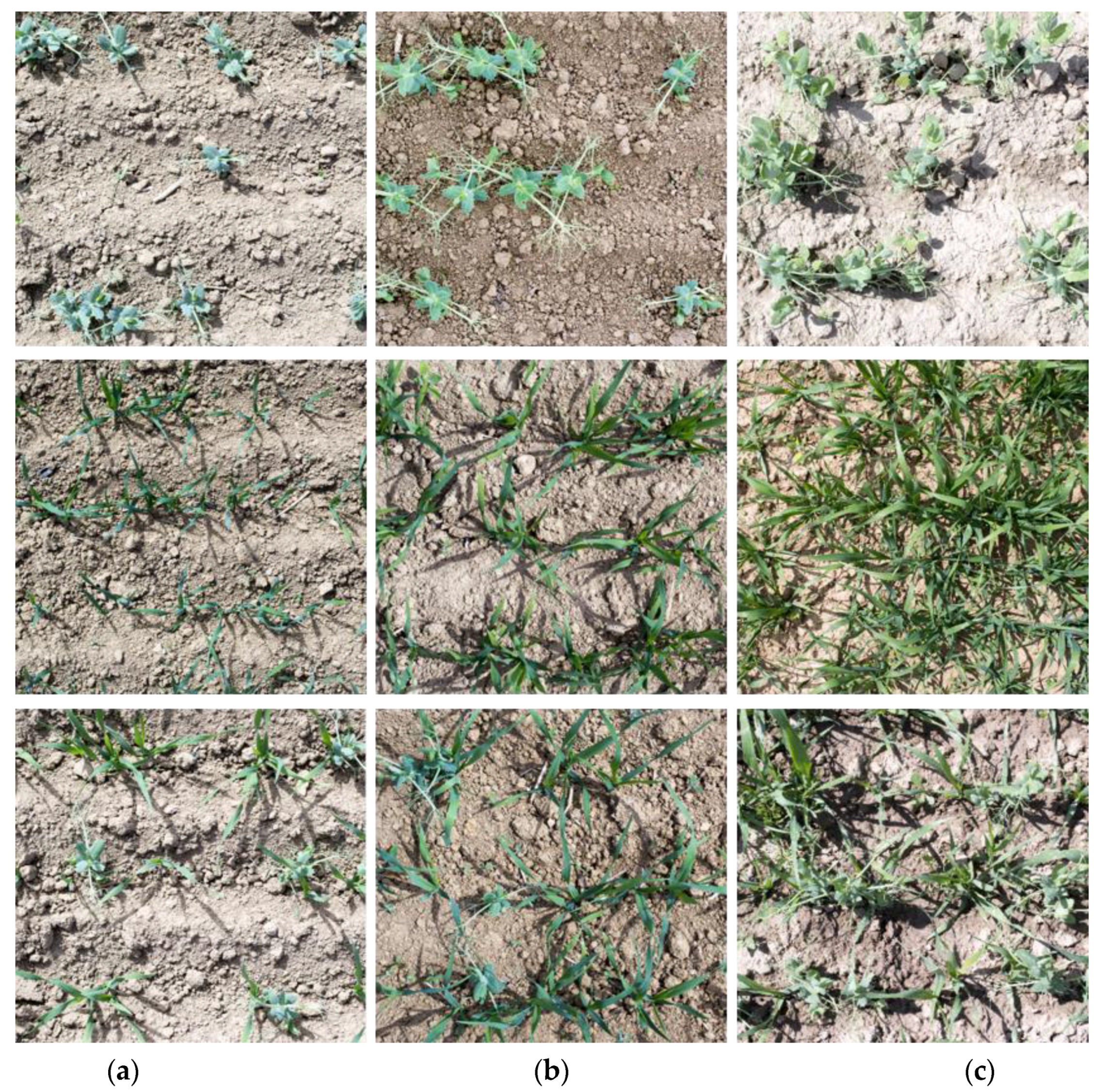
The images were acquired with a D3100 equipped with an AF-S DX NIKKOR 18–55 mm 1:3, 5-5, 6G VR lens (Nikon Corporation, Tokio, Japan) at a distance between 0.5 m and 1 m to capture at least three crop rows in each image. These distances are applicable for moving vehicles like tractors or robots, to automate the image acquisition. The shutter speed was adapted to given illumination conditions and ranged between 1/160 and 1/1250 s with a shorter exposure time under very bright conditions. All the other settings were kept constant (ISO 400, F/8). The image size was 3072 × 4608 pixels with a resolution of 240 dpi. The images had a spatial resolution of 3–6 pixel/mm, depending on the acquisition distance. The images were taken hand-held, i.e., horizontal leveling, and therefore, distance did vary to a certain extent between images. The images were captured along the 80 m of each of the 18 strips, which resulted in a total of 300–400 single images per date. In Figure 2, three exemplary images of the sole and intercrops are shown for the three acquisition dates with different canopy cover, denoted as low, intermediate, and high cover dataset.

2.2. Image Processing and CNN Architecture

For subsequent analysis, first, the software imageJ was used to cut out a section of 2600 × 2600 pixels in the center of each image before processing [29]. Next, these images were analyzed by a semantic CNN to generate the different pixel classes. The output images were afterwards filtered with a Matlab script (Matlab R2019a, The MathWorks Inc., Natick, MA, USA) to get rid of small single objects in binary image results, which corresponded to weeds and other outliers. Therefore, all objects in the binary image with a pixel number smaller than 2400 pixels were removed from the image.
For the semantic segmentation of the acquired images, the online platform of the company Wolution GmbH & Co. KG (Planegg, Germany) was used. They supply an easy and accessible online interface, which could be used to upload, label, and train images with different machine learning algorithms. In our case, we used a semantic CNN based on a deep neural network, similar as described by Havaei et al. [30]. The CNN architecture exploits local and contextual features, and therefore, is able to model the local details and the global context at the same time. The CNN applies a series of layers, constructed from convolutions and activation functions (in this case a rectified linear unit), to the image. In a CNN, each successive layer results in a more abstract feature map, providing more global (contextual) features. The final layer applies a softmax activation function, which results in normalized class probabilities for each pixel in the image. The CNN is trained with the Adam optimizer [31] until the validation loss converges. For this purpose, the dataset is split into 80% training data and 20% validation data.
The Adam optimizer was trained with a learning rate of 10−4. The neural network training was performed with randomly cropped image patches of size 64 × 64 pixels. Each image patch was randomly mirrored and rotated to enlarge the dataset. One batch (for stochastic gradient descent) included 128 image patches, randomly selected from the training images. After each 1000th batch (1000 × 128 image patches), a validation step was performed to check the training error. For validation, 1000 batches from the validation images were randomly selected and evaluated. For the current datasets, we found that the training error converged after about 20 epochs of 1000 batches. In total, the training process took about three hours per dataset.

2.3. CNN Training

The training was done with manually pixel-wise labeled images of pea and oat. The training was performed only with images of single plants of pea and oat. Intercropping images were not used for training. For improving the results, the tendrils and the leaves of pea were labeled into two individual classes. Existing weeds in the images were not labeled, and therefore, were part of the soil/background class. This was possible without a high error rate as the datasets showed a low weed pressure (see Table 1).
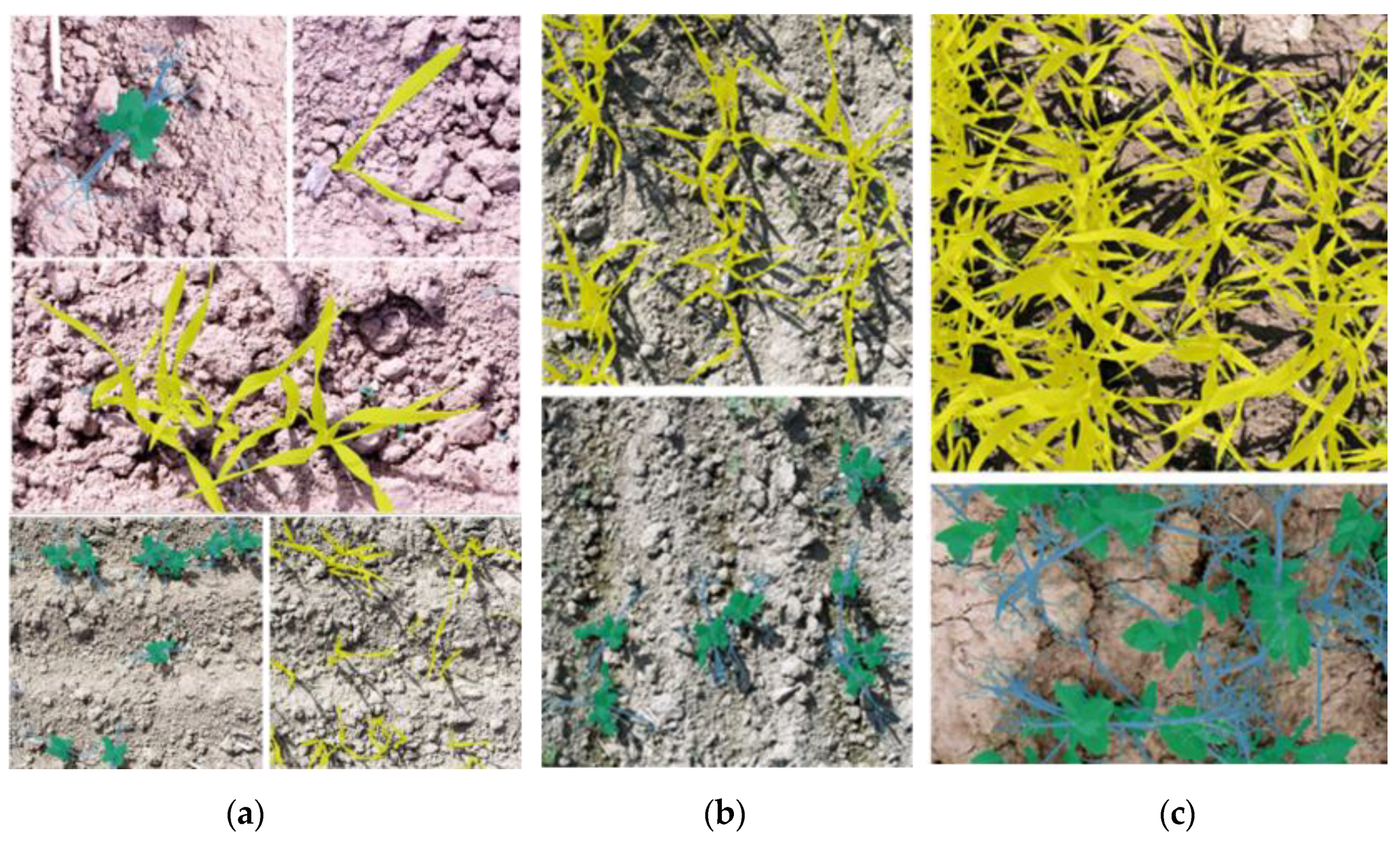
In total, five different networks were trained and evaluated. The first network just used training data from the low cover dataset (LC), the second just from the intermediate cover dataset (IC), and the third just from the high cover dataset (HC). The fourth network combined training data from LC and IC (LC + IC). The fifth network combined all three datasets LC, IC, and HC (LC + IC + HC) for training. Examples of labeled images for the three different networks LC, IC, and HC are shown in Figure 3.
The reason behind this training procedure is that labeling at early growth stages is much less time consuming. It can be partly automated using index-based segmentation as plants overlap only to a small extent. In addition, labeling sole crops is much easier and faster than to differentiate and individually label species in a mixed canopy of an intercropping system.
Therefore, the network input data was ordered from low to high effort for creating the training input. Additionally, the evaluation of the light competition within an intercropping system has to start at an early growth stage with low cover. If we could increase the accuracy of a good working network with just a few additional training images, this could facilitate development time of highly accurate networks for different growth stages.
The idea was to first check the performance of the networks based on each dataset individually, and how the combination of training data influenced the results and robustness. In Table 2, the differently trained networks and their number of input images and plants, and the pixels per class are given in detail. The comparability between the networks individually trained on a specific dataset was assured by a similar number of pea and oat pixels contained in the training images.

2.4. Evaluation

For evaluation, 15 images (each 2600 × 2600 pixels) of each dataset, which were not part of the training data, were randomly selected. From each dataset (low, intermediate, high), five images were selected from each sole crop and the intercrop. Each individual image was divided into three different classes: soil, oat, and pea. The two classes of pea used for training (leaves and tendrils) were combined to compare to ground truth. The results of the CNNs were evaluated with the DPA-Software, which includes a pixel-wise comparison between ground truth image and result [11]. The transferability of the CNNs was evaluated for
(1) The different datasets (low, intermediate, and high cover) by analyzing all three datasets with each of the five trained networks including both sole and intercrops;
(2) The intercrops specifically, by comparing the results achieved for the sole and the intercrops.
For analyzing the accuracy of the networks, the True Positives (TP), False Negatives (FN), and False Positives (FP) for each single class were evaluated and the Precision and Recall were calculated:
P r e c i s i o n = T P T P + F P ,
R e c a l l = T P T P + F N .
Additionally, we calculated the intersection over union (IoU) according to
I o U = | A B | | A B | ,
where A corresponds to the quantity of ground truth pixels and B to the quantity of result pixels of each class.

3. Results and Discussion

First, the performance of the networks over single and intercrop images was tested and evaluated. In all three tested datasets, the classes of oat, pea, and soil pixels were detected at high rates. The networks in general detected oat more reliable than pea in the images. The individually trained networks (LC, IC, and HC) performed best for their corresponding dataset with an average precision of 91% (88–95%) and 75% (64–83%), a recall of 84% (81–89%) and 74% (65–83%), and an Intersection over Union (IoU) of 78% (73–81%) and 60% (48–68%) for oat and pea, respectively (Table 3). The network trained on all datasets (LC + IC + HC) showed almost equal performance and even slightly increased the performance when applied on the intermediate and high cover datasets.
The transfer of the networks to other datasets, especially for the HC-trained network, showed a strong decrease in the mean Intersection over Union (mIoU). The transfer of LC onto the intermediate cover dataset and IC onto the low cover dataset yielded in a mIoU higher than 69%. Whereas, the transfer of LC and IC onto the high cover dataset and the HC onto the other two datasets showed a strong decrease of the mIoU with values between 40% and 50%.
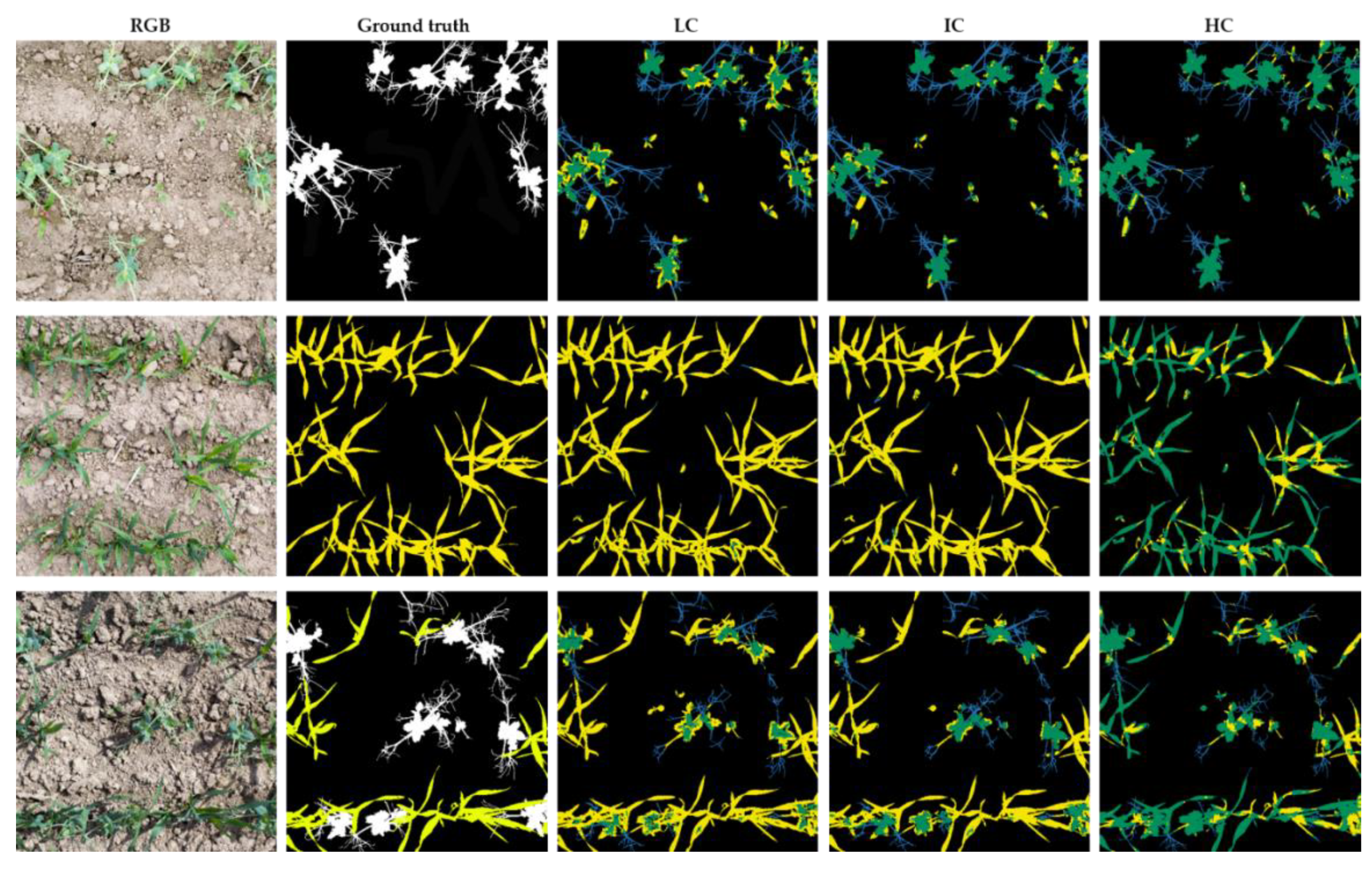
An example for the performance of the three networks individually trained with sole crop images from the three datasets on the intermediate cover dataset is shown in the Figure 4.
These results indicate that the transferability across different growth stages (respectively, degree of canopy cover) is challenging. Therefore, the need for retraining the network for a new dataset seems the only option to optimize the performance. The difference between the accuracy of oat and pea pixels could be a result of the increased complexity of the plant and the overall cover of the two species in the images. Especially in intercropping, the cover of pea was less than half of oat (Table 1). Additionally, the tendrils of pea where hard to detect, especially when their share in cover increased during growth and more tendrils with a small diameter were present. Interestingly, the mIoU dropped considerably for the later growth stage, where overlapping of plants increased and the canopy cover was higher. The main reason for this was the lower quality in detection of the intercrops as shown in Table 4.
The sole crops were detected well across all datasets with an IoU between 72% and 90%. The transfer of the networks trained on sole crop images onto the intercrops showed a good performance for intercropped oat for the first two datasets (IoU: 70–80%). However, the IoU of intercropped pea decreased considerably and for the high cover dataset, the network performed poorly for the intercrops and especially pea.
The largest error was associated with the small tips of the oat plants, which were detected as pea tendrils. The center of the plants resulted in another typical zone of errors. A reason might be shading, which created a different coloration for the center compared with the rest of the plant.
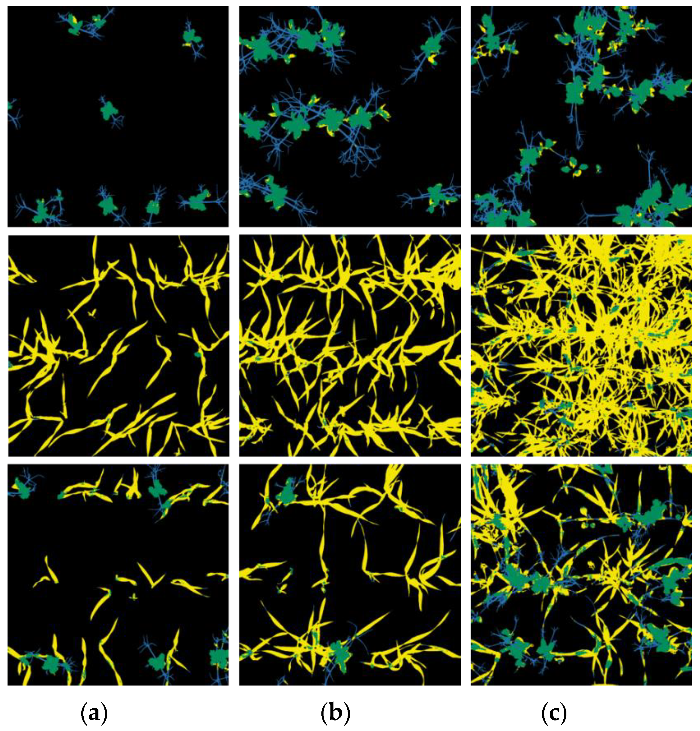
Reasons for this behavior could be the comparable low training input, the change of color, and the different shape of the plants in the high cover dataset as both species reached the next main growth stage (pea: stem elongation, oat: tillering). This leads to the point that future CNN architectures for applications in agriculture should address different growth stages in the networks. To gain a network with the given method that fits all growth stages seems challenging. However, future architectures could address the special needs for extracting invariant features for agricultural plants under different growth stages. The better performance of the LC + IC + HC network on intercropped pea for the high cover dataset indicated that better results might be obtained with more training images of pea. A few example images of this network are shown in the following Figure 5.
For the general use in agriculture, the absolute precision of plant pixels is not mandatory. As todays machines for fertilization and weeding are not plant-specific, mean estimates over the field or a specific site are sufficient. Therefore, the mean crop cover over an area of interest is enough to estimate the light competition between the intercrops for a given agronomic practice (e.g., sowing density of each intercrop) or site. With this in mind, the two best performing networks for each dataset were selected and the mean average cover ( m ¯ ) evaluated by the CNN was compared to the ground truth on an absolute (Δa) and relative (Δr) scale (Table 5).
The results showed that the absolute cover was estimated quite accurately. The maximum absolute difference to ground truth was −1.1% for pea and −5.3% for oat with a relative difference not exceeding 12.1%. The estimated canopy cover of the intercrops were on absolute scale in the same magnitude as the sole crops. However, given their lower canopy cover, relative differences were higher reaching a maximum of 25%. Interestingly, a lower IoU as shown for the high cover dataset (Table 3 and Table 4) does not necessarily result in a lower accuracy of estimated canopy cover.
Compared to the existing state of the art work in the field, the trained networks did perform quite well. The reached mIoU between 66% and 81% for the networks is in the range of published results as mentioned in the introduction. This study confirmed that transferring a CNN to another dataset resulted in a considerable decrease in IoU. This corresponds to the results of Lottes et al. and Bosilj et al. [21,23].
Shorten and Khoshgoftaar highlighted in their review that there are no existing augmentation techniques that can correct a dataset that has a very poor diversity with respect to the test data [27]. However, especially in an agricultural domain, this is the most challenging point, as diversity of the possible real test environment is huge. Therefore, future research has to address the generalization and transferability of networks in the agricultural domain, as we deal with unstructured objects in unstructured environments [25]. Data augmentation techniques like geometric transformations, color space transformations, kernel filters, mixing images, random erasing, feature space augmentation, adversarial training, generative adversarial network-based augmentation, neural style transfer, and meta-learning schemes could help to gain better transferability of networks in the future.

4. Conclusions

The results of this study showed that it is feasible to estimate the canopy cover in intercropping systems with a satisfying accuracy based on sole crop training data. However, the transferability of trained networks onto other datasets—than the one used for training—has to be improved in future research to reduce the effort for retraining the networks for new situations. In a next step, the network will also be trained with another dataset having a higher weed pressure to estimate weed cover separately (not as a part of the soil/background class). Besides the use of the estimated canopy cover to analyze light competition between intercrops and identify promising management practices, a combination of the results with site-specific management would open new possibilities to dynamically influence the interactions between crop species to maximize yield and weed suppression.

Author Contributions

Conceptualization, S.M. and D.R.; formal analysis, S.M. and D.R.; funding acquisition, S.M.; methodology, S.M. and D.R.; project administration, S.M.; software, D.R.; validation, S.M. and D.R.; visualization, S.M. and D.R.; writing—original draft, S.M. and D.R.; writing—review & editing, S.M. and D.R. All authors have read and agreed to the published version of the manuscript.

Funding

This research was funded by the European Union’s Horizon 2020 Programme for Research & Innovation under grant agreement n°727217 (ReMIX: Redesigning European cropping systems based on species MIXtures).

Acknowledgments

We thank Jonas Boysen for helping with preparing the ground truth data, Alexander Stana and Nils Lüling for proofreading, and Julian Zachmann and the technical staff of the research station for managing the field experiment. Additionally, we thank Dominik Wuttke and Moritz Münchmeyer for their help and support while preparing this manuscript.

Conflicts of Interest

The authors declare no conflict of interest.

References

  1. Vandermeer, J. The Ecology of Intercropping, 1st ed.; Cambridge University Press: Cambridge, UK, 1989; ISBN 0521345928. [Google Scholar]
  2. Jensen, E.S.; Bedoussac, L.; Carlsson, G.; Journet, E.; Justes, E.; Hauggaard-Nielsen, H. Enhancing Yields in Organic Crop Production by Eco-Functional Intensification. Sustain. Agric. Res. 2015, 4, 42–50. [Google Scholar] [CrossRef]
  3. Verret, V.; Pelzer, E.; Bedoussac, L.; Jeu, M. Tracking on-farm innovative practices to support crop mixture design: The case of annual mixtures including a legume crop. Eur. J. Agron. 2020, 115. [Google Scholar] [CrossRef]
  4. Hauggaard-Nielsen, H.; Gooding, M.; Ambus, P.; Corre-Hellou, G.; Crozat, Y.; Dahlmann, C.; Dibet, A. Pea-Barley intercropping for efficient symbiotic N2-fixation, soil N acquisition and use of other nutrients in European organic cropping systems. Field Crop. Res. 2009, 113, 64–71. [Google Scholar] [CrossRef]
  5. Jensen, E.S. Intercropping of grain legumes and cereals improves the use of soil N resources and reduces the requirement for synthetic fertilizer N: A global-scale analysis. Agron. Sustain. Dev. 2020, 40, 1–9. [Google Scholar] [CrossRef] [Green Version]
  6. Bedoussac, L.; Journet, E.; Hauggaard-Nielsen, H.; Naudin, C.; Corre-Hellou, G.; Jensen, E.S. Ecological principles underlying the increase of productivity achieved by cereal-grain legume intercrops in organic farming. A review. Agron. Sustain. Dev. 2015, 35, 911–935. [Google Scholar] [CrossRef]
  7. Gaudio, N.; Escobar-Gutiérrez, A.J.; Casadebaig, P.; Evers, J.B.; Gérard, F.; Louarn, G.; Colbach, N.; Munz, S.; Launay, M.; Marrou, H.; et al. Current knowledge and future research opportunities for modeling annual crop mixtures. A review. Agron. Sustain. Dev. 2019, 39, 1–20. [Google Scholar] [CrossRef] [Green Version]
  8. Munz, S.; Graeff-Hönninger, S.; Lizaso, J.I.; Chen, Q.; Claupein, W. Modeling light availability for a subordinate crop within a strip-intercropping system. Field Crop. Res. 2014, 155, 77–89. [Google Scholar] [CrossRef]
  9. Shepherd, M.J.; Lindsey, L.E.; Lindsey, A.J. Soybean Canopy Cover Measured with Canopeo Compared with Light Interception. Agric. Environ. Lett. 2018, 3, 1–3. [Google Scholar] [CrossRef] [Green Version]
  10. Kusumam, K.; Kranjík, T.; Pearson, S.; Cielniak, G.; Duckett, T. Can You Pick a Broccoli? 3D-Vision Based Detection and Localisation of Broccoli Heads in the Field. In Proceedings of the 2016 IEEE International Conference on Intelligent Robots and Systems (IROS), Daejeon, Korea, 9–14 October 2016; pp. 646–651. [Google Scholar]
  11. Riehle, D.; Reiser, D.; Griepentrog, H.W. Robust index-based semantic plant/background segmentation for RGB-images. Comput. Electron. Agric. 2020, 169, 105201. [Google Scholar] [CrossRef]
  12. Åstrand, B.; Baerveldt, A.J. An agricultural mobile robot with vision-based perception for mechanical weed control. Auton. Robots 2002, 13, 21–35. [Google Scholar] [CrossRef]
  13. Kamilaris, A.; Prenafeta-Boldú, F.X. Deep learning in agriculture: A survey. Comput. Electron. Agric. 2018, 147, 70–90. [Google Scholar] [CrossRef] [Green Version]
  14. Lottes, P.; Hoeferlin, M.; Sander, S.; Stachniss, C. An Effective Classification System for Separating Sugar Beets and Weeds for Precision Farming Applications. In Proceedings of the IEEE International Conference on Robotics and Automation (ICRA), Stockholm, Sweden, 16–21 May 2016; pp. 5157–5163. [Google Scholar]
  15. Milioto, A.; Lottes, P.; Stachniss, C. Real-time Semantic Segmentation of Crop and Weed for Precision Agriculture Robots Leveraging Background Knowledge in CNNs. In Proceedings of the IEEE International Conference on Robotics and Automation (ICRA), Brisbane, QLD, Australia, 21–25 May 2018; pp. 2229–2235. [Google Scholar]
  16. Bargoti, S.; Underwood, J. Image Segmentation for Fruit Detection and Yield Estimation in Apple Orchards. J. Field. Robot. 2016, 34, 1–22. [Google Scholar] [CrossRef] [Green Version]
  17. Dias, P.A.; Tabb, A.; Medeiros, H. Multispecies fruit flower detection using a refined semantic segmentation network. IEEE Robot. Autom. Lett. 2018, 3, 3003–3010. [Google Scholar] [CrossRef] [Green Version]
  18. Sankaran, S.; Mishra, A.; Ehsani, R.; Davis, C. A review of advanced techniques for detecting plant diseases. Comput. Electron. Agric. 2010. [Google Scholar] [CrossRef]
  19. Reiser, D.; Vázquez-Arellano, M.; Paraforos, D.S.; Garrido-Izard, M.; Griepentrog, H.W. Iterative individual plant clustering in maize with assembled 2D LiDAR data. Comput. Ind. 2018, 99. [Google Scholar] [CrossRef]
  20. Krogh Mortensen, A.; Dyrmann, M.; Karstoft, H.; Nyholm Jorgensen, R.; Gislum, R. Semantic Segmentation of Mixed Crops using Deep Convolutional Neural Network. In Proceedings of the CIGR-AgEng Conference, Aarhus, Denmark, 26–29 June 2016; pp. 1–6. [Google Scholar]
  21. Lottes, P.; Behley, J.; Milioto, A.; Stachniss, C. Robust joint stem detection and crop—Weed classification using image sequences for plant—Specific treatment in precision farming. J. Field Robot. 2020, 37, 20–34. [Google Scholar] [CrossRef]
  22. Dutta, A.; Gitahi, J.M.; Ghimire, P.; Mink, R.; Peteinatos, G.; Engels, J.; Hahn, M.; Gerhards, R. Weed Detection in Close-range Imagery of Agricultural Fields using Neural Networks. Publ. DGPF 2018, 27, 633–645. [Google Scholar]
  23. Bosilj, P.; Duckett, T. Transfer learning between crop types for semantic segmentation of crops versus weeds in precision agriculture. J. Field Robot. 2020, 37, 7–19. [Google Scholar] [CrossRef]
  24. Reiser, D.; Vázquez-Arellano, M.; Izard, M.G.; Paraforos, D.S.; Sharipov, G.; Griepentrog, H.W. Clustering of Laser Scanner Perception Points of Maize Plants. Adv. Anim. Biosci. 2017, 8, 204–209. [Google Scholar] [CrossRef] [Green Version]
  25. Taylor, L.; Nitschke, G. Improving Deep Learning with Generic Data Augmentation. In Proceedings of the 2018 IEEE Symposium Series on Computational Intelligence (SSCI), Bangalore, India, 18–21 November 2018; pp. 1542–1547. [Google Scholar]
  26. Bechar, A.; Vigneault, C. Agricultural robots for field operations: Concepts and components. Biosyst. Eng. 2016, 149, 94–111. [Google Scholar] [CrossRef]
  27. Shorten, C.; Khoshgoftaar, T.M. A survey on Image Data Augmentation for Deep Learning. J. Big Data 2019, 6, 60. [Google Scholar] [CrossRef]
  28. Meier, U. Growth Stages of Mono- and Dicotyledonous Plants; BBCH Monograph, Open Agrar Repositorium; Blackwell Wissenschafts-Verlag: Berlin, Germany, 2018; ISBN 9783955470715. [Google Scholar]
  29. Software, I. Open Source Software ImagJ. 2019. Available online: https://imagej.net/Welcome (accessed on 1 May 2020).
  30. Mohammad, H.; Axel, D.; David, W.; Antoine, B.; Aaron, C.; Yoshua, B.; Chris, P.; Pierre-Marc, J.; Hugo, L. Brain tumor segmentation with Deep Neural Networks. Med. Image Anal. 2017, 35, 18–31. [Google Scholar]
  31. Kingma, D.P.; Ba, J. Adam: A Method for Stochastic Optimization. arXiv 2014, arXiv:1412.6980. [Google Scholar]
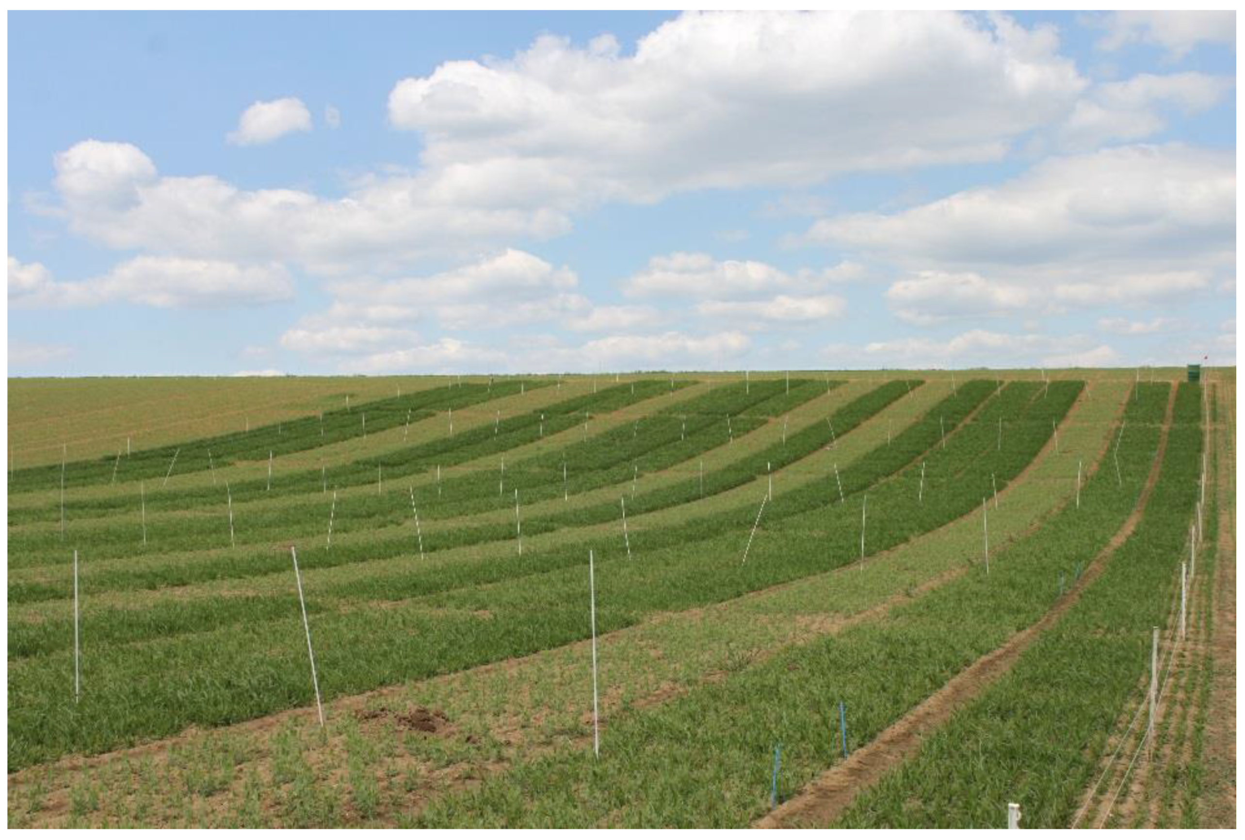
Figure 1. Overview of the field experiment. The first three strips from right to left are oat, pea–oat intercrop, and pea.
Agriculture 10 00354 g001
Figure 2. Exemplary images of the three datasets used for the evaluation. (a) Low cover dataset (25 April), (b) intermediate cover dataset (2 May), and (c) high cover dataset (16 May). From top to bottom: pea, oat, and pea–oat intercrops.
Agriculture 10 00354 g002
Figure 3. Examples of labeled images for training of the three networks: (a) low cover (LC), (b) intermediate cover (IC), and (c) high cover (HC). Three classes were labeled: pea leaves (green), pea tendrils (blue), and oat plants (yellow).
Agriculture 10 00354 g003
Figure 4. Examples for images from the intermediate cover dataset analyzed by the three individually trained networks. From top to bottom: pea, oat, and pea–oat intercrops (yellow: oat, green: pea, blue: pea tendrils, white: pea combined).
Agriculture 10 00354 g004
Figure 5. Examples for images from the three datasets: (a) low, (b) intermediate, and (c) high cover analyzed by the network trained on all datasets (LC + IC + HC). From top to bottom: pea, oat, and pea–oat intercrops (yellow: oat, green: pea, blue: pea tendrils).
Agriculture 10 00354 g005
Table 1. Mean values of the canopy cover of pea, oat, and weed in sole crops and intercrops for the three datasets.
DateName of DatasetCover in Sole Crops [%]Cover in Intercrops [%]
PeaOatWeedPeaOatWeed
25 AprilLow cover7.014.10.43.87.90.6
2 MayIntermediate cover10.120.71.24.813.01.4
16 MayHigh cover17.651.81.911.430.32.0
Table 2. Description of the training input for the five networks.
Low Cover (LC)Intermediate Cover (IC)High Cover (HC)LC + ICLC + IC + HC
No. of images42774956
No. of pea plants1024039142181
No. of oat plants1589864256320
Pea pixels 3.628.5372.518.8752.129.7946.147.4128.277.206
Oat pixels3.473.4503.456.2334.020.4416.929.68310.950.124
Soil pixels87.489.75941.344.8905.614.212128.834.649134.448.861
Table 3. Intersection over union (IoU, %), precision (%), and recall (%) for pea, oat, and soil for the three evaluation datasets (low cover—LC, intermediate cover—IC, and high cover—HC) each analyzed by the five different networks. Individually trained networks in bold.
DatasetNetworkIoU [%]Precision [%]Recall [%]
mIoUSoilPeaOatSoilPeaOatSoilPeaOat
Low CoverLC81.196.767.779.197.978.795.198.782.982.5
IC69.194.155.857.595.865.197.998.279.658.2
HC41.485.630.28.491.931.998.092.685.38.4
LC + IC77.796.160.776.497.378.393.998.873.080.3
LC + IC + HC81.196.667.978.797.977.495.598.784.781.8
Int. CoverLC75.593.555.677.396.881.882.596.563.592.4
IC80.394.964.581.497.182.590.297.774.789.3
HC46.080.731.825.589.333.688.689.485.226.3
LC + IC75.893.655.977.896.677.785.896.966.689.3
LC + IC + HC81.495.166.582.597.781.688.397.378.392.6
High CoverLC50.364.235.850.776.840.787.979.775.254.5
IC40.159.533.027.969.137.895.181.171.928.3
HC66.378.647.572.986.564.388.189.664.580.9
LC + IC41.358.130.135.870.434.190.976.971.737.1
LC + IC + HC67.578.151.173.388.362.386.287.174.183.0
Table 4. Intersection over union (IoU, %) of pea and oat in sole crops and intercrops for the three evaluation datasets (low, intermediate, and high cover) each analyzed by the individually trained network (LC, IC, HC) and the network trained on all datasets (LC + IC + HC).
DatasetNetworkSole CropsIntercrops
Pea IoU [%]Oat IoU [%]Pea IoU [%]Oat IoU [%]
Low CoverLC81.783.160.273.7
LC + IC + HC82.284.358.370.4
Int. CoverIC76.586.652.679.6
LC + IC + HC76.689.756.879.9
High CoverHC74.482.125.663.3
LC + IC + HC72.382.738.564.2
Table 5. Mean estimated canopy cover ( m ¯ ) of pea and oat in sole crops and intercrops and absolute (Δa) and relative (Δr) difference to ground truth for the three evaluation datasets (low, intermediate, and high cover).
DatasetNetworkSole CropsIntercrops
Pea Cover [%]Oat Cover [%]Pea Cover [%]Oat Cover [%]
m ¯ ΔaΔr m ¯ ΔaΔr m ¯ ΔaΔr m ¯ ΔaΔr
Low CoverLC + IC + HC6.3−0.7−10.012.6−1.5−10.64.70.923.76.2−1.7−21.5
LC6.2−0.8−11.412.4−1.7−12.14.30.513.26.5−1.4−17.7
Int. CoverLC + IC + HC9.5−0.6−5.920.6−0.1−0.54.3−0.5−10.413.20.21.5
IC9.3−0.8−7.919.2−1.5−7.23.6−1.2−25.013.00.00.0
High CoverLC + IC + HC17.0−0.6−3.450.5−1.3−2.513.82.421.128.1−2.2−7.3
HC16.5−1.1−6.346.5−5.3−10.29.3−2.1−18.429.1−1.2−4.0
Mean ( m ¯ ) LC + IC + HC −0.6−6.4 −1.0−4.5 0.911.5 −1.2−9.1
single net −0.9−8.5 −2.8−9.8 −0.9−10.1 −0.9−7.2