Tobacco Plant Detection in RGB Aerial Images


Abstract
1. Introduction
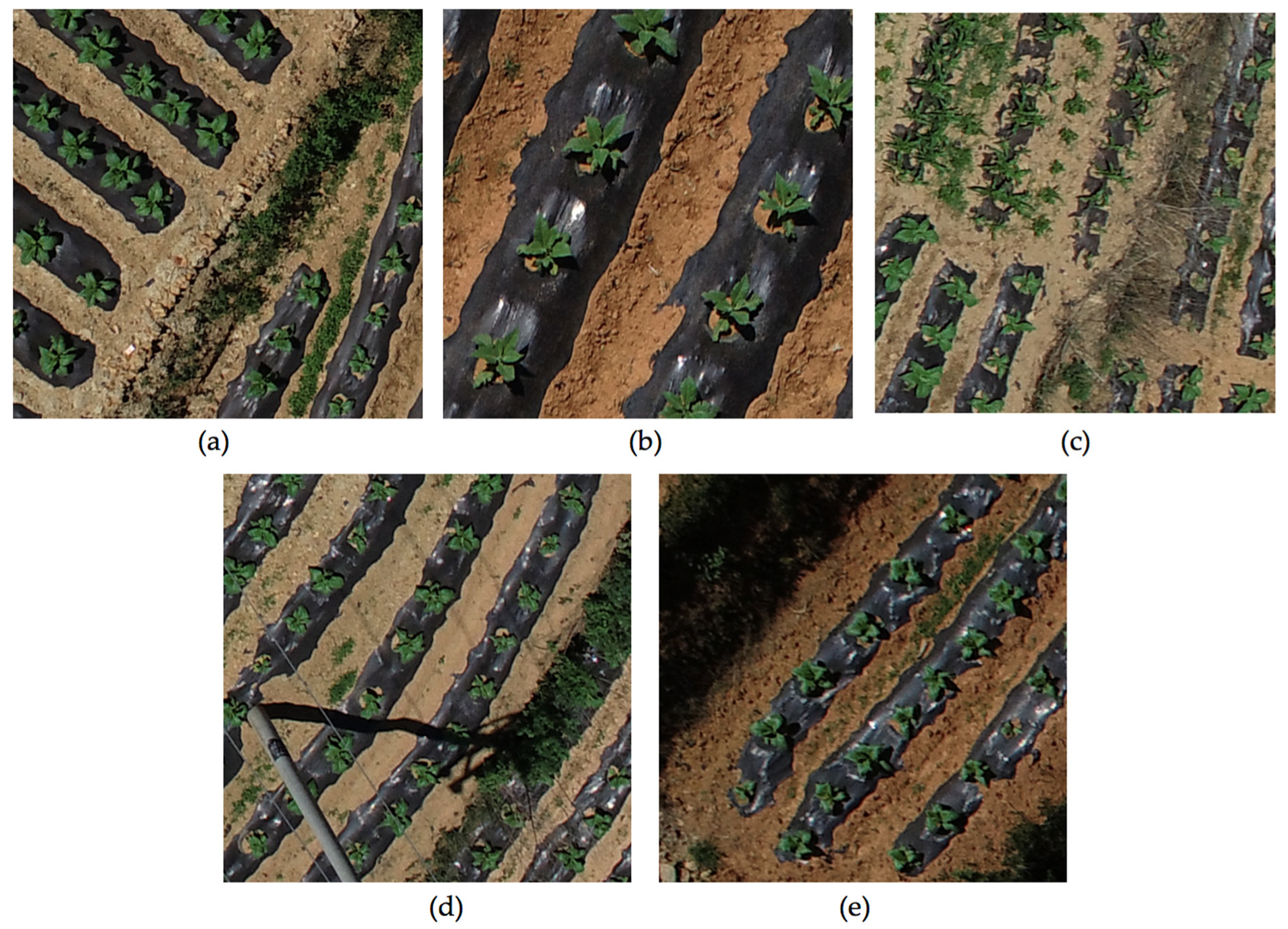
2. Materials
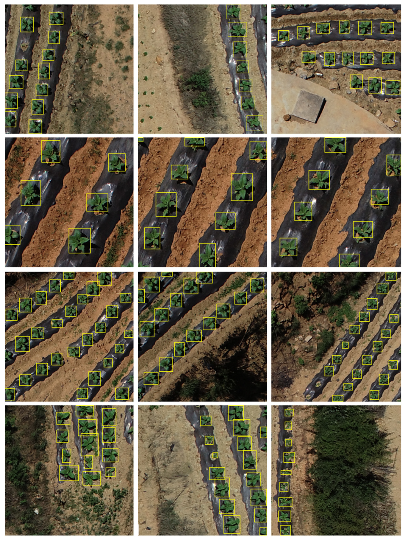
2.1. Data Annotation
2.2. Data Augmentation
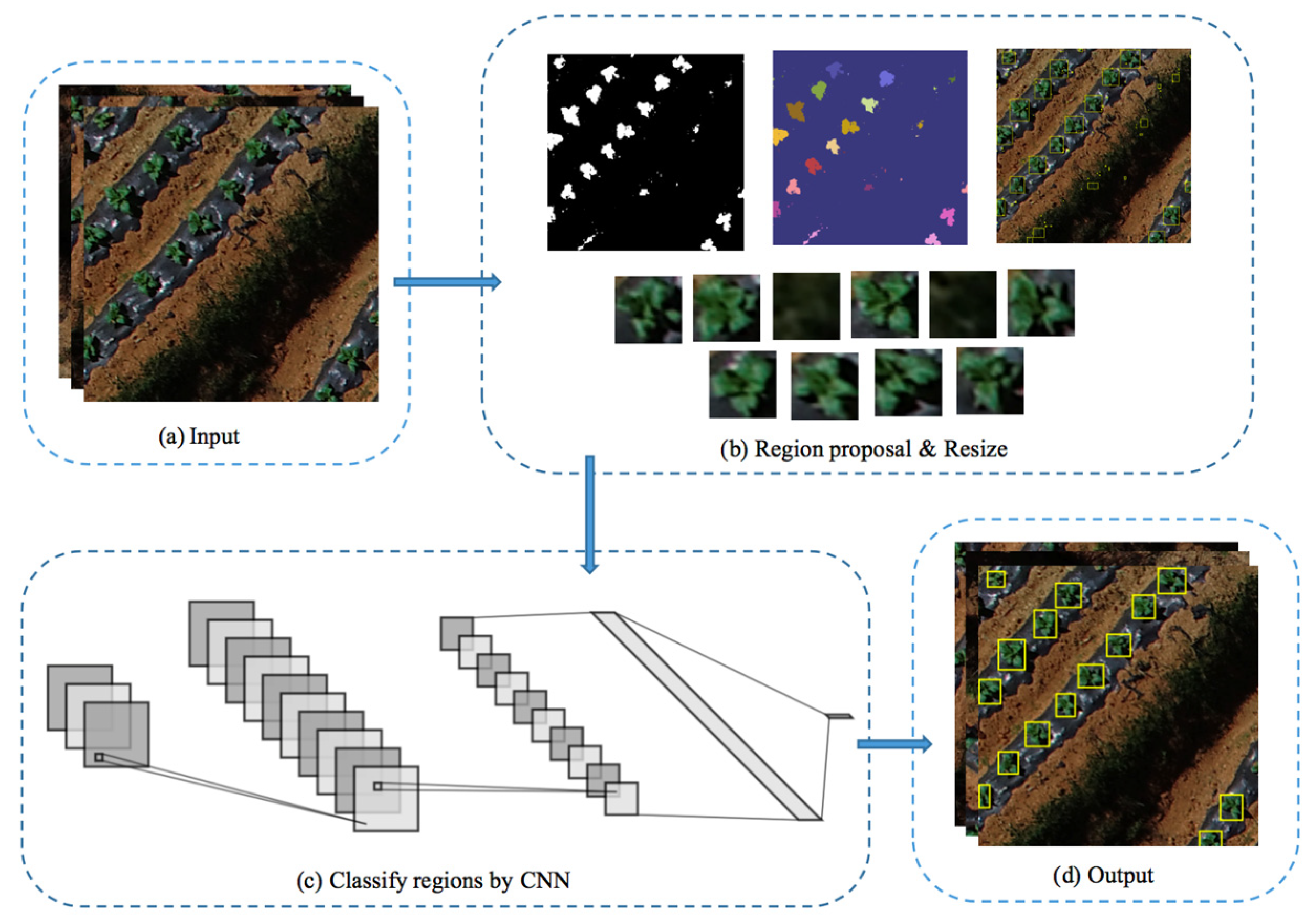
3. Methods
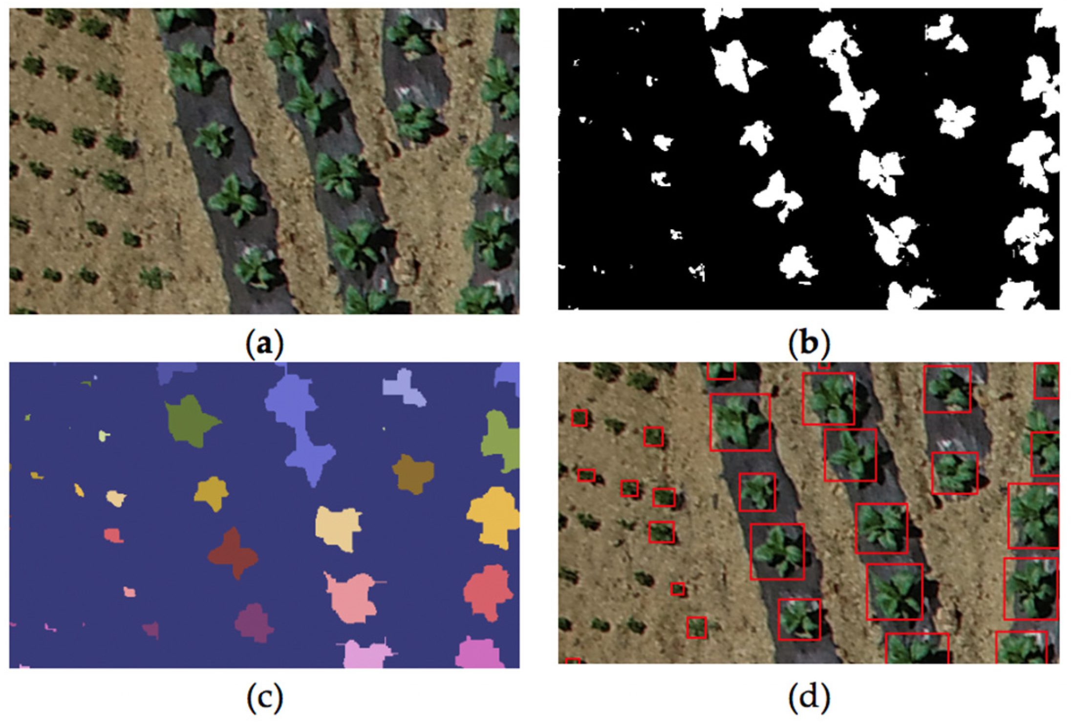
3.1. Candidates Selecting Algorithm
3.1.1. Binarization
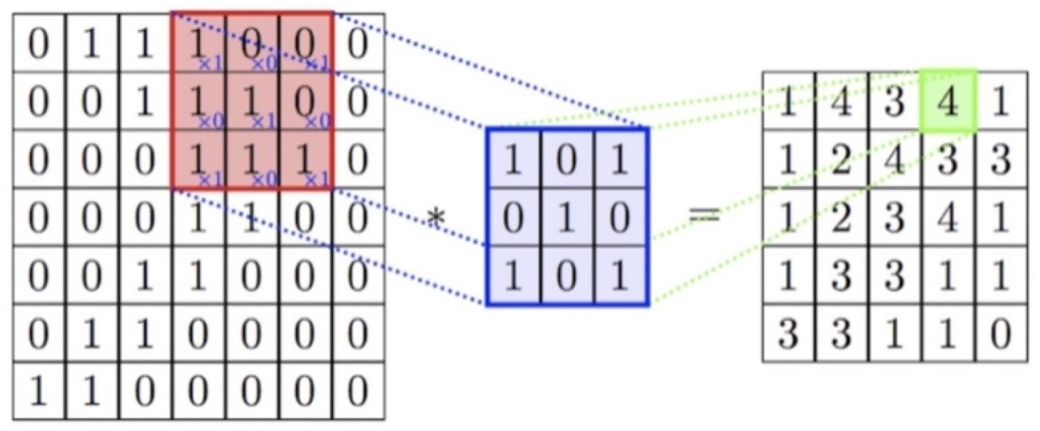
3.1.2. Grouping
3.1.3. Extraction and Resizing
3.2. Neural Network
3.2.1. Layers in CNNs
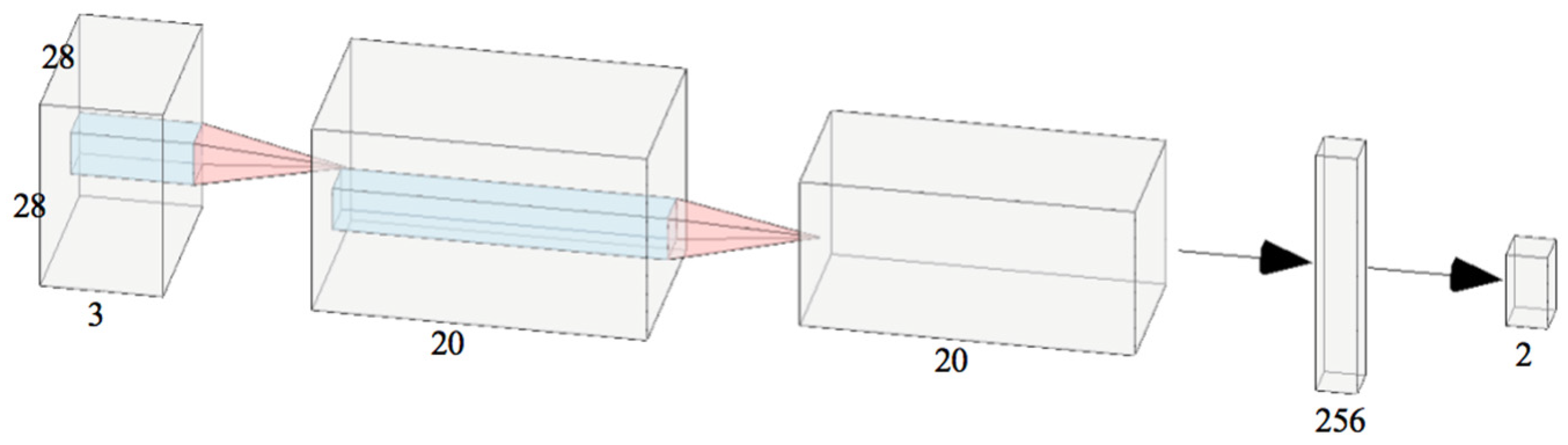
3.2.2. Network Architecture
- The convolutional layer has 20 filters of size pixels. The inputs are padded with zero, and the stride of filter is one. We use ReLU as its activation function. This layer is supposed to extract features of the input.
- The previous layer’s output is a matrix of size . It is processed here by a pooling layer whose pool size is , and its stride is two. After the pooling process we have mentioned in the last paragraph, the feature map is down sampled to half of its original size.
- Former max pooling layer outputs matrix of size . Before it is inputted into the fully connected layer, it needs to be flattened. Thus, right after the max pooling layer is a layer that flattens the matrix into a vector with a dimensionality of 3920.
- The first fully connected layer contains 256 neurons. It is activated by ReLU, as well.
- The second fully connected layer contains two neurons and it is activated by SoftMax function. It outputs a two-dimensional vector, where the first dimension indicates the input’s probability of being a tobacco plant, and the second dimension indicates the probability of a nontobacco plant.
3.2.3. Training of Network
4. Experiments and Results
4.1. Environment
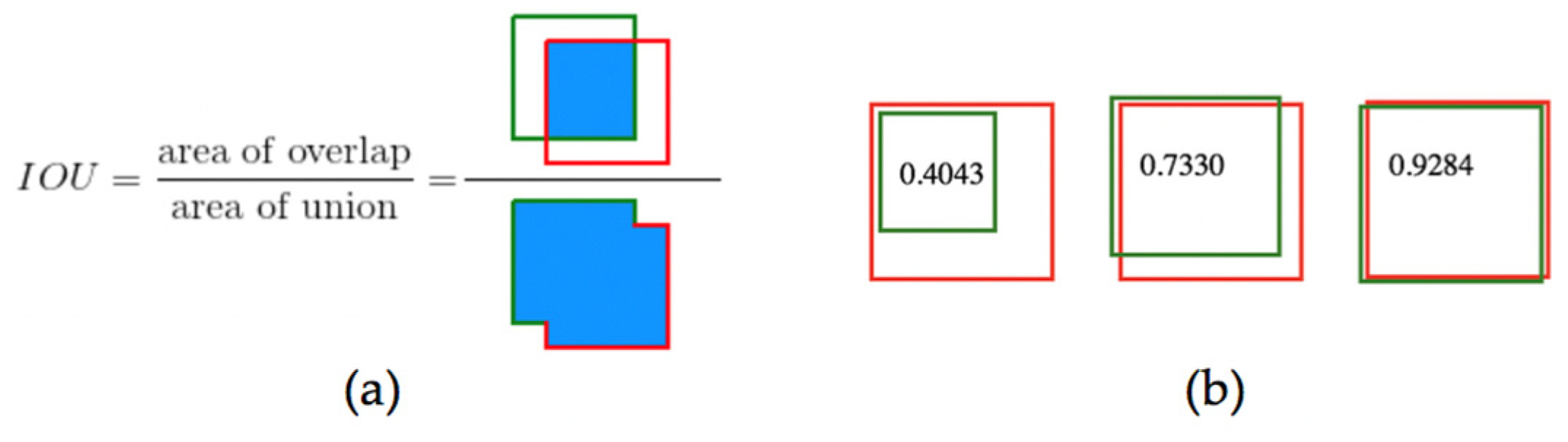
4.2. Metrics
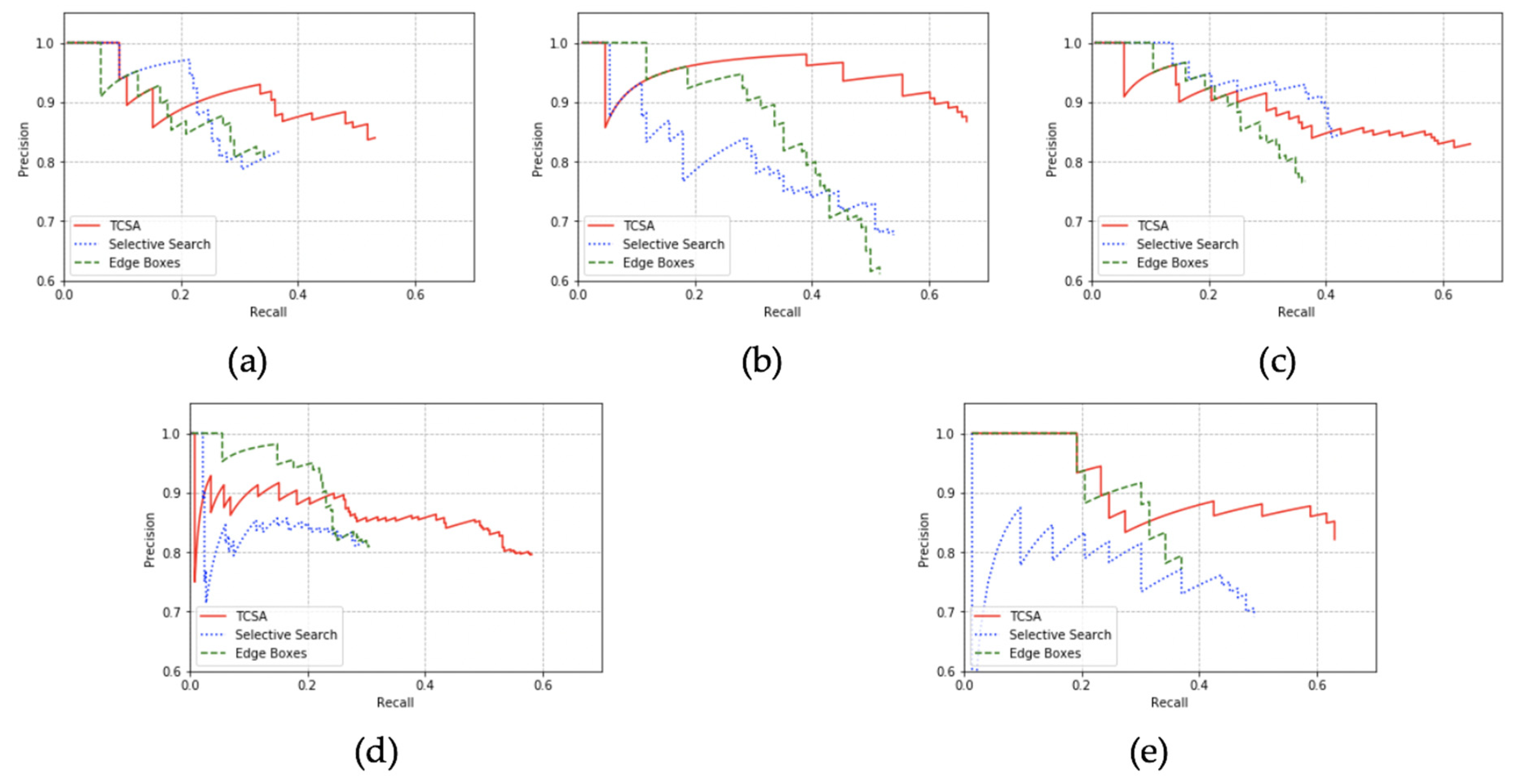
4.3. Evaluation on Region Proposal Algorithms
- TCSA reaches the best recall over the five datasets. The average recall rate of our region proposed method is 18% higher than selective search and 22% higher than edge boxes.
- TCSA also gets the best AP over the datasets. The average AP of TCSA is 18% higher than selective search and 21% higher than edge boxes.
- The precision of TCSA is averagely 5% higher than selective search and 7 % better than edge boxes. However, selective search reaches better precision on some of the datasets where selective search outputs fewer predictions to guarantee its precision. Selective search’s precision is guaranteed by its segmentation process and in further studies we will attempt to take that as a reference to improve the precision of TCSA.
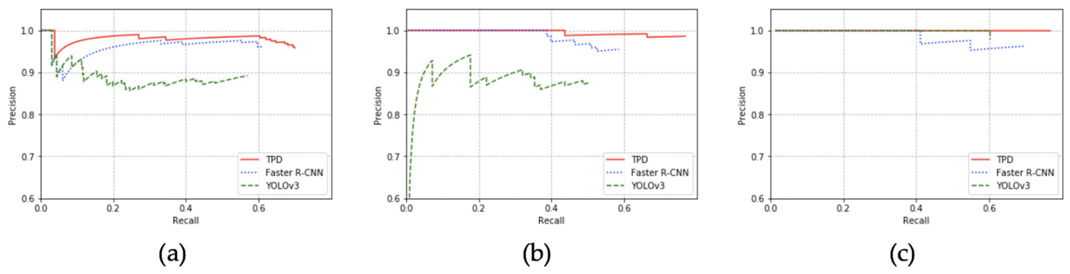
4.4. Evaluation on Detection Systems
- TPD reaches the best recall over all of the testing datasets. On average, the recall is 12.5% higher than faster R-CNN and 21% higher than YOLOv3.
- The precision of TPD is averagely 8% higher than faster R-CNN and 7% higher than YOLOv3. However, TPD has a slightly lower precision on dataset 3 than faster R-CNN which should be caused by TCSA’s lower precision on this dataset.
- TPD gets the best AP over the datasets, as well. Averagely, it is 16% higher than faster R-CNN and 23% higher than YOLOv3.
5. Conclusions
Author Contributions
Funding
Acknowledgments
Conflicts of Interest
References
- Musk, A.W.; De Klerk, N.H. History of tobacco and health. Respirology 2003, 8, 286–290. [Google Scholar] [CrossRef] [PubMed]
- Fiore, M.C.; Bailey, W.C.; Cohen, S.J.; Dorfman, S.F.; Goldstein, M.G.; Gritz, E.R.; Heyman, R.B.; Jaen, C.R.; Kottke, T.E.; Lando, H.A.; et al. Treating Tobacco Use and Dependence: Clinical Practice Guideline Respiratory Care; U.S. Department of Health and Human Services: Irving, TX, USA, 2008.
- Stein, M.; Bargoti, S.; Underwood, J. Image based mango fruit detection, localisation and yield estimation using multiple view geometry. Sensors 2016, 16, 1915. [Google Scholar] [CrossRef] [PubMed]
- Bargoti, S.; Underwood, J.P. Image segmentation for fruit detection and yield estimation in apple orchards. J. Field Robot. 2017, 34, 1039–1060. [Google Scholar] [CrossRef]
- Ferencz, C.; Bognar, P.; Lichtenberger, J.; Hamar, D.; Tarcsai, G.; Timár, G.; Molnár, G.; Pásztor, S.; Steinbach, P.; Székely, B.; et al. Crop yield estimation by satellite remote sensing. Int. J. Remote Sens. 2004, 25, 4113–4149. [Google Scholar] [CrossRef]
- Prasad, A.K.; Chai, L.; Singh, R.P.; Kafatos, M. Crop yield estimation model for Iowa using remote sensing and surface parameters. Int. J. Appl. Earth Obs. Geoinf. 2006, 8, 26–33. [Google Scholar] [CrossRef]
- Fan, Z.; Lu, J.; Gong, M.; Xie, H.; Goodman, E.D. Automatic tobacco plant detection in UAV images via deep neural networks. IEEE J. Sel. Top. Appl. Earth Obs. Remote Sens. 2018, 11, 876–887. [Google Scholar] [CrossRef]
- Felzenszwalb, P.F.; Girshick, R.B.; McAllester, D.; Ramanan, D. Object detection with discriminatively trained part-based models. IEEE Trans. Pattern Anal. Mach. Intell. 2009, 32, 1627–1645. [Google Scholar] [CrossRef]
- Dalal, N.; Triggs, B. Histograms of oriented gradients for human detection. In Proceedings of the 2005 IEEE Computer Society Conference on Computer Vision and Pattern Recognition (CVPR’05), San Diego, CA, USA, 20–25 June 2005. [Google Scholar]
- Suykens, J.A.; Vandewalle, J. Least squares support vector machine classifiers. Neural Process. Lett. 1999, 9, 293–300. [Google Scholar] [CrossRef]
- Fares, M.A.; Elena, S.F.; Ortiz, J.; Moya, A.; Barrio, E. A sliding window-based method to detect selective constraints in protein-coding genes and its application to RNA viruses. J. Mol. Evol. 2002, 55, 509–521. [Google Scholar] [CrossRef] [PubMed]
- Yang, L.; Yang, G.; Yin, Y.; Xiao, R. Sliding window-based region of interest extraction for finger vein images. Sensors 2013, 13, 3799–3815. [Google Scholar] [CrossRef] [PubMed]
- Alexe, B.; Deselaers, T.; Ferrari, V. Measuring the objectness of image windows. IEEE Trans. Pattern Anal. Mach. Intell. 2012, 34, 2189–2202. [Google Scholar] [CrossRef] [PubMed]
- Uijlings, J.R.; Van De Sande, K.E.; Gevers, T.; Smeulders, A.W. Selective search for object recognition. Int. J. Comput. Vis. 2013, 104, 154–171. [Google Scholar] [CrossRef]
- Zitnick, C.L.; Dollár, P. Edge boxes: Locating object proposals from edges. In European Conference on Computer Vision; Springer: Berlin/Heidelberg, Germany, 2014; pp. 391–405. [Google Scholar]
- Krizhevsky, A.; Sutskever, I.; Hinton, G.E. Imagenet classification with deep convolutional neural networks. In Proceedings of the Advances in Neural Information Processing Systems, Lake Tahoe, NV, USA, 3–6 December 2012; pp. 1097–1105. [Google Scholar]
- Girshick, R.; Donahue, J.; Darrell, T.; Malik, J. Rich feature hierarchies for accurate object detection and semantic segmentation. In Proceedings of the IEEE Conference on Computer Vision and Pattern Recognition, Columbus, OH, USA, 23–28 June 2014; pp. 580–587. [Google Scholar]
- Girshick, R. Fast r-cnn. In Proceedings of the IEEE International Conference on Computer Vision, Santiago, Chile, 7–13 December 2015; pp. 1440–1448. [Google Scholar]
- Ren, S.; He, K.; Girshick, R.; Sun, J. Faster r-cnn: Towards real-time object detection with region proposal networks. In Proceedings of the Advances in Neural Information Processing Systems, Montreal, QC, Canada, 7–12 December 2015; pp. 91–99. [Google Scholar]
- He, K.; Gkioxari, G.; Dollár, P.; Girshick, R. Mask r-cnn. In Proceedings of the IEEE International Conference on Computer Vision, Venice, Italy, 22–29 October 2017; pp. 2961–2969. [Google Scholar]
- Redmon, J.; Divvala, S.; Girshick, R.; Farhadi, A. You only look once: Unified, real-time object detection. In Proceedings of the IEEE Conference on Computer Vision and Pattern Recognition, Las Vegas, NV, USA, 26–30 June 2016; pp. 779–788. [Google Scholar]
- Redmon, J.; Farhadi, A. Yolov3: An incremental improvement. arXiv 2018, arXiv:1804.02767. [Google Scholar]
- Shafiee, M.J.; Chywl, B.; Li, F.; Wong, A. Fast YOLO: A fast you only look once system for real-time embedded object detection in video. arxiv 2017, arXiv:1709.05943. [Google Scholar] [CrossRef]
- Zhong, J.; Lei, T.; Yao, G. Robust vehicle detection in aerial images based on cascaded convolutional neural networks. Sensors 2017, 17, 2720. [Google Scholar] [CrossRef] [PubMed]
- Beamer, S.; Asanovic, K.; Patterson, D. Direction-optimizing breadth-first search. Sci. Program. 2013, 21, 137–148. [Google Scholar] [CrossRef]
- Arlia, D.; Coppola, M. Experiments in parallel clustering with DBSCAN. In Lecture Notes in Computer Science, Proceedings of the European Conference on Parallel Processing, Manchester, UK, 28–31 August 2001; Springer: Berlin/Heidelberg, Germany, 2001; pp. 326–331. [Google Scholar]
- Simonyan, K.; Zisserman, A. Very deep convolutional networks for large-scale image recognition. arXiv 2014, arXiv:1409.1556. [Google Scholar]
- He, K.; Zhang, X.; Ren, S.; Sun, J. Deep residual learning for image recognition. In Proceedings of the IEEE Conference on Computer Vision and Pattern Recognition, Las Vegas, NV, USA, 26–30 June 2016; pp. 770–778. [Google Scholar]
- Scherer, D.; Müller, A.; Behnke, S. Evaluation of pooling operations in convolutional architectures for object recognition. In Lecture Notes in Computer Science, Proceedings of the International Conference on Artificial Neural Networks, Thessaloniki, Greece, 15–18 September 2010; Springer: Berlin/Heidelberg, Germany, 2010; pp. 92–101. [Google Scholar]
- Jang, E.; Gu, S.; Poole, B. Categorical reparameterization with gumbel-softmax. arXiv 2016, arXiv:1611.01144. [Google Scholar]
- LeCun, Y.; Jackel, L.; Bottou, L.; Brunot, A.; Cortes, C.; Denker, J.; Drucker, H.; Guyon, I.; Muller, U.; Sackinger, E.; et al. Comparison of learning algorithms for handwritten digit recognition. In Proceedings of the International Conference on Artificial Neural Networks, Perth, Australia, 27–30 November 1995; Volume 60, pp. 53–60. [Google Scholar]
- Nair, V.; Hinton, G.E. Rectified linear units improve restricted boltzmann machines. In Proceedings of the 27th International Conference on Machine Learning (ICML-10), Haifa, Israel, 21–24 June 2010; pp. 807–814. [Google Scholar]
- Faster R-CNN Implemented with Python. Available online: https://github.com/rbgirshick/py-faster-rcnn (accessed on 5 February 2015).
- Yolov3 a Keras implementation of YOLOv3 (Tensorflow Backend). Available online: https://github.com/qqwweee/keras-yolo3 (accessed on 3 April 2018).
- Davis, J.; Goadrich, M. The relationship between Precision-Recall and ROC curves. In Proceedings of the 23rd International Conference on Machine Learning. ACM, Pittsburgh, PA, USA, 25–29 June 2006; pp. 233–240. [Google Scholar]


| Keras | TensorFlow | Numpy | OpenCV |
|---|---|---|---|
| 2.1.6 | 1.10.0 | 1.14.5 | 4.1.2 |
| Datasets | Algorithms | AP | Time(s) |
|---|---|---|---|
| Dataset1 | BFS | 0.4916 | 0.0049 |
| DBSCAN | 0.4964 | 0.2273 | |
| Dataset2 | BFS | 0.6393 | 0.0043 |
| DBSCAN | 0.6260 | 0.2264 | |
| Dataset3 | BFS | 0.5804 | 0.0043 |
| DBSCAN | 0.5613 | 0.1490 | |
| Dataset4 | BFS | 0.5104 | 0.0039 |
| DBSCAN | 0.5312 | 0.1791 | |
| Dataset5 | BFS | 0.5806 | 0.0036 |
| DBSCAN | 0.5958 | 0.1390 | |
| Average | BFS | 0.5604 | 0.0041 |
| DBSCAN | 0.5621 | 0.1841 |
| Datasets | Algorithms | TP | FP | FN | Recall | Precision | AP |
|---|---|---|---|---|---|---|---|
| Dataset1 | TCSA | 84 | 16 | 74 | 0.5316 | 0.8400 | 0.4916 |
| Selective Search | 60 | 11 | 98 | 0.3797 | 0.8451 | 0.3543 | |
| Edge Boxes | 55 | 12 | 103 | 0.3481 | 0.8209 | 0.3205 | |
| Dataset2 | TCSA | 85 | 13 | 43 | 0.6641 | 0.8673 | 0.6393 |
| Selective Search | 71 | 31 | 57 | 0.5547 | 0.6961 | 0.4606 | |
| Edge Boxes | 66 | 42 | 62 | 0.5156 | 0.6111 | 0.4586 | |
| Dataset3 | TCSA | 117 | 24 | 64 | 0.6464 | 0.8298 | 0.5804 |
| Selective Search | 76 | 14 | 105 | 0.4199 | 0.8444 | 0.4003 | |
| Edge Boxes | 66 | 20 | 115 | 0.3646 | 0.7674 | 0.3368 | |
| Dataset4 | TCSA | 211 | 54 | 152 | 0.5813 | 0.7962 | 0.5104 |
| Selective Search | 107 | 24 | 256 | 0.2948 | 0.8168 | 0.2535 | |
| Edge Boxes | 111 | 26 | 252 | 0.3058 | 0.8102 | 0.2874 | |
| Dataset5 | TCSA | 46 | 10 | 27 | 0.6301 | 0.8214 | 0.5806 |
| Selective Search | 36 | 16 | 37 | 0.4932 | 0.6923 | 0.4010 | |
| Edge Boxes | 27 | 8 | 46 | 0.3699 | 0.7714 | 0.3492 |
| Datasets | Algorithms | TP | FP | FN | Recall | Precision | AP |
|---|---|---|---|---|---|---|---|
| TPD | 254 | 11 | 109 | 0.6997 | 0.9585 | 0.6903 | |
| Dataset3 | Faster R-CNN | 221 | 9 | 142 | 0.6088 | 0.9609 | 0.5945 |
| YOLOv3 | 207 | 25 | 156 | 0.5702 | 0.8922 | 0.5163 | |
| TPD | 139 | 2 | 42 | 0.7680 | 0.9858 | 0.7646 | |
| Dataset4 | Faster R-CNN | 106 | 5 | 75 | 0.5856 | 0.9550 | 0.5791 |
| YOLOv3 | 91 | 13 | 90 | 0.5028 | 0.8750 | 0.4574 | |
| TPD | 56 | 0 | 17 | 0.7671 | 1.0000 | 0.7671 | |
| Dataset5 | Faster R-CNN | 51 | 2 | 22 | 0.6986 | 0.9623 | 0.6896 |
| YOLOv3 | 44 | 1 | 29 | 0.6027 | 0.9778 | 0.6027 |
© 2020 by the authors. Licensee MDPI, Basel, Switzerland. This article is an open access article distributed under the terms and conditions of the Creative Commons Attribution (CC BY) license (http://creativecommons.org/licenses/by/4.0/).
Share and Cite
Sun, X.; Peng, J.; Shen, Y.; Kang, H. Tobacco Plant Detection in RGB Aerial Images. Agriculture 2020, 10, 57. https://doi.org/10.3390/agriculture10030057
Sun X, Peng J, Shen Y, Kang H. Tobacco Plant Detection in RGB Aerial Images. Agriculture. 2020; 10(3):57. https://doi.org/10.3390/agriculture10030057
Chicago/Turabian StyleSun, Xingping, Jiayuan Peng, Yong Shen, and Hongwei Kang. 2020. "Tobacco Plant Detection in RGB Aerial Images" Agriculture 10, no. 3: 57. https://doi.org/10.3390/agriculture10030057
APA StyleSun, X., Peng, J., Shen, Y., & Kang, H. (2020). Tobacco Plant Detection in RGB Aerial Images. Agriculture, 10(3), 57. https://doi.org/10.3390/agriculture10030057