Article

Downscaling Regional Crop Yields to Local Scale Using Remote Sensing

by
Paresh B. Shirsath
1,*,
Vinay Kumar Sehgal
2 and
Pramod K. Aggarwal
1
1
CGIAR Research Program on Climate Change, Agriculture and Food Security (CCAFS), Borlaug Institute for South Asia (BISA), International Maize and Wheat Improvement Centre (CIMMYT), New Delhi 110012, India
2
Division of Agricultural Physics, Indian Agricultural Research Institute (IARI), ICAR, New Delhi 110012, India
*
Author to whom correspondence should be addressed.
Agriculture 2020, 10(3), 58; https://doi.org/10.3390/agriculture10030058
Submission received: 26 January 2020 / Revised: 7 February 2020 / Accepted: 10 February 2020 / Published: 2 March 2020

Abstract

:
Local-scale crop yield datasets are not readily available in most of the developing world. Local-scale crop yield datasets are of great use for risk transfer and risk management in agriculture. In this article, we present a simple method for disaggregation of district-level production statistics over crop pixels by using a remote sensing approach. We also quantified the error in the disaggregated statistics to ascertain its usefulness for crop insurance purposes. The methodology development was attempted in Parbhani district of Maharashtra state with wheat and sorghum crops in the winter season. The methodology uses the ratio of Enhanced Vegetation Index (EVI) of pixel to total EVI of the crop pixels in that district corresponding to the growth phase of the crop. It resulted in the generation of crop yield maps at the 500 m resolution pixel (grid) level. The methodology was repeated to generate time-series maps of crop yield. In general, there was a good correspondence between disaggregated crop yield and sub-district level crop yields with a correlation coefficient of 0.9.

1. Introduction

Crop production statistics are vital to agricultural planning and policy design and play an important role in the planning and allocation of inputs for the development of the agricultural sector. In an agrarian country, like India, where agriculture is still the main source of livelihood, crop production statistics are even more important. In India, crop area statistics and crop yield statistics are reported using different methods based on the state institutional mechanism. The crop production statistics are being collected at different scales. These statistics are often available at the district scale and to some extent at the sub-district scale. The district/sub-district scale is probably good for the planning of agricultural inputs where the majority of these transactions happen, and also for setting up the minimum support price and for national/international selling/procurement decisions. Recently, the crop insurance schemes were launched in India at the village scale and it required village level time-series of yields [1]. The major challenge in implementation is the absence of historical yield series at the village level. In order to undertake effective implementation of a crop insurance scheme with creditability, there is a need to produce a consistent long time-series of historical crop yield data at the local scale (such as village), which may be useful for fixing key insurance metrics like threshold yield and indemnity level. There have been only some piecemeal studies in India on the use of technologies for yield estimation and insurance contract design. The evidence base of these technologies, under diverse agro-ecological regions of the country, is also limited to support implementation in crop insurance programs [1]. Besides insurance, several new information and communications technologies are emerging that deliver targeted and actionable advisories to farmers [2], and the absence of village level yield series is one of the key limitations. Estimating or measuring yields at the field level is of great use to farmers, service dealers, commodity traders, and policy-makers.
Several methods have been tried to estimate or forecast crop yields at different resolutions. These methods can be classified into various categories or types based on how they model yield. The process can be date driven or process based. In a data driven approach where empirical models are built based on observed data, such models analyse data and fit equation(s) to the data. These models are often regarded as black-box (e.g., artificial neural network-based models) since they do not provide explanations on the mechanism that drives the yield [3]. The process-based models, unlike empirical models, provide detailed information on crop growth and penology on a daily basis. The yield modelling tools are dominated by crop forecasting tools and early warning systems [4,5] and operational crop yield forecasting systems [5,6,7]. There are several spatial crop-modelling systems available, like Monitoring Agricultural ResourceS (MARS), CCAFS Regional Agricultural Forecasting Toolbox (CRAFT), Geospatial Simulation (GeoSIM). These spatial crop modelling systems generate high-resolution yield surfaces (1 × 1 km: MARS, 10 × 10 km: CRAFT), which then can be used as a substitute for local scale yields. These models need detailed databases on weather, soil, crop cultivars, and management practices. Often getting these datasets at the required granularity is a challenge. Among the models successfully used to simulate crop yield in India are InfoCrop [8,9,10,11], DSSAT [12,13], APSIM [14], CERES [15,16,17], CropSyst [17], ORYZA [18], and many others. Most of these model applications focused on understanding the climate change impacts on crop productivity [10,11,13,15]. In addition to crop modelling [8,9,16], several other methods, like weather based models and satellite data driven yield models [19,20], are commonly used for monitoring crop growth and yield. Crop yield estimation using remote sensing remained a widely researched topic and several detailed reviews are also available on it [21,22,23,24]. Most of the remote sensing approaches used Normalized Difference Vegetation Index (NDVI) as a key parameter in crop yield estimation [19]. Many of the remote sensing based methods often follow an integrated approach, which essentially combines crop growth simulation models, weather data, remote sensing data, and scalable models [25,26]. Crop masking is one of the important input parameters to demarcate a crop boundary for simulation, which can be achieved by employing different classification techniques using remote sensing data [26,27]. All inputs for crop growth simulation models (masked with crop growing areas) and simulated yields are used to develop statistical models for different combinations of possible image acquisition dates, and these are then applied to high spatial resolution and gridded weather data [28,29,30]. These methods, however, require huge input datasets and are often challenging to implement. Downscaling yields to the desired level using these methods will need high resolution climatological, remote sensing, and biophysical datasets, which are not readily available. These methods also fail to incorporate or validate existing productions statistics, which are often available and being used. Considering the acceptance of the district-level crop production statistics and the fact that there is an institutional mechanism in place for collection of this data, it is required to fuse the methodologies that use these reported statistics for the purpose of attaining downscaled statistics at the required administrative level.
In this study, a simple downscaling approach is presented for generating a time-series yield of multiple crops at the local scale by disaggregating the district scale yield/production statistics using remote sensing data. We also quantified the error in the disaggregated statistics to ascertain its usefulness for crop insurance purposes. The pixel level yields generated here can add vital information to the implementation of insurance schemes and contingency planning at a disaggregated level. The methodology development part is attempted in the Parbhani district of Maharashtra State with two crops in the winter (rabi) crop season. We understand that the study lacks the validation with the ground truth measurements of crop yield and area, and it is likely that the performance of this approach might not be similar for other crops, especially in the rainy season where the availability of quality remote sensing data is low.

2. Materials and Methods

2.1. Study District and Crops

The study was undertaken for the Parbhani district (Figure 1) of Maharashtra State of India. The Parbhani district is spread over ~650,000 ha with 9 sub-districts (tehsils/taluks) and 848 villages (https://parbhani.gov.in/village_list/ accessed on 25 January 2020). The Parbhani district is slightly larger in terms of area compared to the average Indian district area of ~450,000 ha. This district is in a hot semi-arid ecological region with an average annual rainfall of 830 mm (http://maharain.gov.in/ accessed on 25 January 2020). In Parbhani, cotton, sorghum, soybean, and green gram are the key crops in the rainy season (kharif) and wheat and sorghum in the winter season. In this study, we attempted the disaggregation of winter (rabi) crops of Jowar (sorghum) and wheat. The district level crop statistics for the Parbhani district for 1999–2000 to 2010–2011 period were downloaded from the website of Department of Agriculture and Cooperation, Ministry of Agriculture and Farmers’ Welfare, Govt. of India (https://aps.dac.gov.in/APY/Index.htm accessed on 25 January 2020). Owing to an overlap of the agricultural calendar (June to May in next year) and the crop area, production statistics are often referred to with the current and next calendar year (e.g., 2001–2002 for agriculture year starting in 2001). The sub-district level (tehsil/taluk) level crop area and yield statistics were collected from the Office of Commissionerate of Agriculture, Maharashtra State, Pune. The sub-district level statistics were used for cross validating the accuracy/error of disaggregation of district level crop statistics.

2.2. Satellite Datasets

In order to meet the requirement of generating a long time-series of yield statistics, we used the Terra-MODIS (Moderate Resolution Imaging Spectrometer) derived 500 m Vegetation Indices (VIs) image product for the 2000–2001 to 2013–2014 period (14 years) at a frequency of 16 days in this study. A total of 322 VI image products pertaining to the study area (MODIS Granule h25v7) were downloaded through the USGS Global Visualization Viewer (http://glovis.usgs.gov/). MODIS VI Image Product: Global MOD13A1 (version 5) image products are generated and provided every 16 days at a 500-m spatial resolution as a gridded level-3 product in the Sinusoidal projection. Each file contains four reflectance band images (blue, red, near infrared, and mid infrared) and two vegetation indices images (NDVI and EVI). Global MODIS vegetation indices are designed to provide consistent spatial and temporal comparisons of vegetation conditions. Blue, red, and near-infrared reflectance, centred at 469, 645, and 858-nanometers, respectively, are used to determine the MODIS daily vegetation indices. The daily vegetation index images are composited for 16 days to produce a maximum value composite (MVC) VI image for the 16-day period. This study also used the Enhanced Vegetation Index (EVI) times-series images for classification of crop types and disaggregation of crop yields. EVI is an ‘optimised’ index designed to enhance the vegetation signal with improved sensitivity in high biomass regions. EVI is more responsive to canopy structural variations, including leaf area index (LAI), canopy type, plant physiognomy, and canopy architecture [31]. It thus supports improved vegetation monitoring through a de-coupling of the canopy background signal and a reduction in atmosphere influences.

2.3. Methodology

The overall methodology followed in this study is depicted as a flow chart in Figure 2. The steps shown in the first column are those related to the acquisition and pre-processing of satellite data. The steps shown in the second column are those related to the identification of pixels of the crop of interest in a season in the study districts. The steps shown in the third column are those related to finding a weighting criterion using satellite derived index to distribute district crop statistics over the identified crop pixels. Then, the distributed crop statistics are re-aggregated at the sub-district, i.e., the tehsil/taluk level, and compared with the reported values for an error analysis of the disaggregated values. Based on this methodology, a time-series of disaggregated yield statistics were generated for the 2000–2001 to 2013–2014 period. The methodology is described for these three columns in subsequent sections.

2.3.1. Pre-Processing of Satellite Data

The pre-processing of time-series of MODIS image granules was carried out in ENVI™ + IDL™ V4.8 Image Processing software. Each MODIS Granule in HDF-EOS format was imported into native binary format of Image Processing Software, and among the scientific datasets present in the granule, only the EVI image dataset was extracted. All the 322 extracted EVI images in original sinusoidal projection were stacked together in a time-series starting from Julian day 129 of 2000 (9-May-2000) to Julian day 113 of 2014 (23-April-2014). The Julian day of an EVI image refers to the starting day of the 16-day period. The stacked images were reprojected from Sinusoidal projection to Lambert Conformal Conic (LCC) projection with WGS-84 datum and a pixel size of 500 m using nearest neighbour resampling method. The stacked EVI images were subsetted, corresponding to the geographical extent of the study district. The original image stores scaled EVI values in integer. By applying the scale factor for recalibration, the images were converted into true EVI values in float.

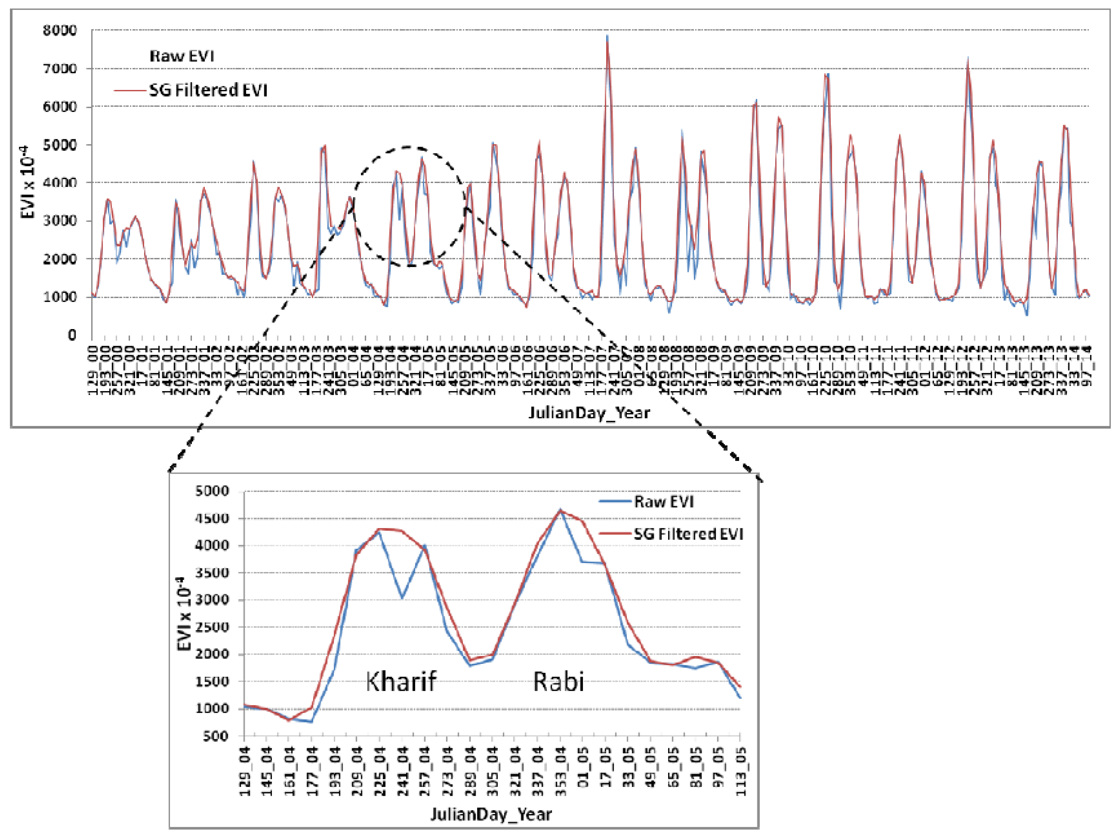
EVI Time-Series Filtering

Although the 16-day maximum value compositing of EVI is implemented to minimise the noise due to cloud contamination, it has been reported that the VI signal is still contaminated by significant residual noise due to atmospheric variability and bi-directional effects [32,33]. Such residual noise is more prominent under Indian conditions, especially during the rainy (kharif) season, when cloudy conditions persist for months together. These noises greatly undermine the basic assumption that the changes in VI are related to changes in vegetation conditions, thus affecting the monitoring of land cover and terrestrial ecosystems [34,35]. For this reason, a number of methods for reducing noise and constructing high-quality VI time-series data sets for further analysis have been formulated, applied, and evaluated.
Among the different methods proposed in literature, we adopted an algorithm-based Savitzky–Golay filter, to efficiently reduce the contamination in the VI time-series that is caused primarily by cloud contamination and atmospheric variability. The algorithm is mainly based on the approach proposed by Chen et al., 2004. This method is based on two assumptions: (1) that the VI data from a satellite sensor is primarily related to vegetation changes and follows annual cycle of growth and decline; and (2) that clouds and poor atmospheric conditions mostly reduce VI values, requiring that sudden drops in VI, which are not compatible with the gradual process of vegetation change, be regarded as noise and removed. This algorithm makes the data approach the upper VI envelope and to best fit the VI variations over the season through an iterative process. At the heart of the algorithm is the Savitzky–Golay filter, which is a weighted moving average filter with weighting given as a polynomial of a certain degree (3rd degree in this case). The weight coefficients, when applied to a signal, perform a polynomial least squares fit within the filter window. This polynomial is designed to preserve higher moments within the data and to reduce the bias introduced by the filter. We cross-checked the filter (Savitzky–Golay) output for inconsistencies on a sample basis. Please see Figure 3, where we highlight the raw and filtered EVI profile over 14 years.
The blue coloured profile shows noises in terms of sudden dips in data, while the filtered red colour profile fits the outer EVI envelope, is smoothened, and preserves the periods of growth and decline well.

2.3.2. Crop Area Identification

Crop area estimation methodology and its efficacy depends on various operational factors, such as land configuration, field shape, crop type, cropping pattern, available skills, and resources [36]. Here, we used the Hierarchical Decision Rule method for crop area identification based on the growth profile of EVI. The scientific rationale for separability of different landuse/crop classes using hierarchical decision rules is based on using the a-priori knowledge of the temporal spectral growth profiles of the various land covers including crops [37]. MODIS Vegetation Image Product was used in the study, and the EVI values ranged from −2000 to +10,000 with a scale factor of 0.0001. In the first step, the pixels, which were masked out during filtering, were labelled as “Non-crop”. In the next step, the current fallow pixels with an EVI below 0.2 during November, as well as Early February periods, were identified. The current fallow represents the agricultural land where sowing has not been done in the current season. Then, the pixels with wheat crop were identified based on the decision that the EVI profile shows a peak anywhere between January and February. Using the decision rule classification above, the winter (rabi) season crops were classified for each crop season of this study.

Land Cover Image

The global MODIS/Terra + Aqua Land Cover Type (MCD12Q1 product for h25v7 granule) for the year 2012 period, available from http://reverb.echo.nasa.gov/ at a resolution of 500 m in sinusoidal projection and HDF-EOS format, was downloaded. The first layer in the IGBP Land Cover Type Classification with sixteen classes was extracted and reprojected. The global land use layer was subsetted, corresponding to the bounds of the study area (Figure 4a). The grids with land use class of Cropland (class = 12) was retained and other land-use classes were masked out. The croplands mask was overlaid with a study area boundary to generate the cropland mask of the study area. The croplands land use mask for the study area is shown in Figure 4b.

2.3.3. Disaggregation of District Yield Statistics

Weighing criterion: The basic premise we adopted in this study to disaggregate district statistics over the crop pixels of interest was that the integrated EVI for the growth period of the crop is directly related to the crop yield. The higher the value of integrated EVI, the higher the crop yield will be. In order to scale this relation, a weighting factor (F) was calculated as the ratio of “Crop pixel integrated EVI” to the “Total integrated EVI over all the Crop pixels in the district”.
F = E V I p i x e l E V I d i s t r i c t
where, EVIpixel is the integrated EVI value of the pixel of the crop of interest, EVIdistrict is the sum of EVIpixel over all the crop pixels in that district, i.e.,
E V I d i s t r i c t = i = 0 n E V I p i x e l
where, the total number of pixels of the crop of interest in the district is n. So, an F value map for crop pixel was calculated.
As the EVIdistrict was an integrated value, we correspondingly disaggregated district wise crop production statistics over the crop pixels, instead of district yield statistics. For a crop pixel, the F value was multiplied by the district production statistics and divided by the pixel area (i.e., 25 ha), to arrive at the yield value of the crop at the pixel level in kg/ha.
Y i e l d p i x e l = F × P d i s t r i c t A
where, Pdistrict is the district crop production in (kg), and A is the area of one pixel in (ha).

3. Results

3.1. Crop Mapping

The decision tree approach was allied to generate crop maps for each year. Figure 5 shows the classified map of the Parbhani district for the rabi season year 2010–2011 as an example; this map was generated by inputting time-series of 13 filtered EVI bands between 14-September-2010 and 22-March-2011.
In order to verify the classification accuracy, the wheat and rabi sorghum crop area was aggregated at the sub-district (tehsil/taluk) level and compared with the statistics reported by the State Department of Agriculture. The comparison for the year 2010–2011 is shown in Figure 6. The error in the remote sensing (RS) estimated area of wheat as compared to values reported by the State Department of Agriculture (SDA) varied between a −17.6% underestimation for the Parbhani sub-district (tehsil/taluk) to a 12.0% overestimation in the Selu sub-district (tehsil/taluk). Overall, at the district level, the error was a 3.6% underestimation. The error in remote sensing estimated that the rabi sorghum area at the sub-district (tehsil/taluk) level varied between −11.0% in the Manwat sub-district (tehsil/taluk) to +20% in the Pathri sub-district (tehsil/taluk), with an overall 1.0% overestimation error at the district level.

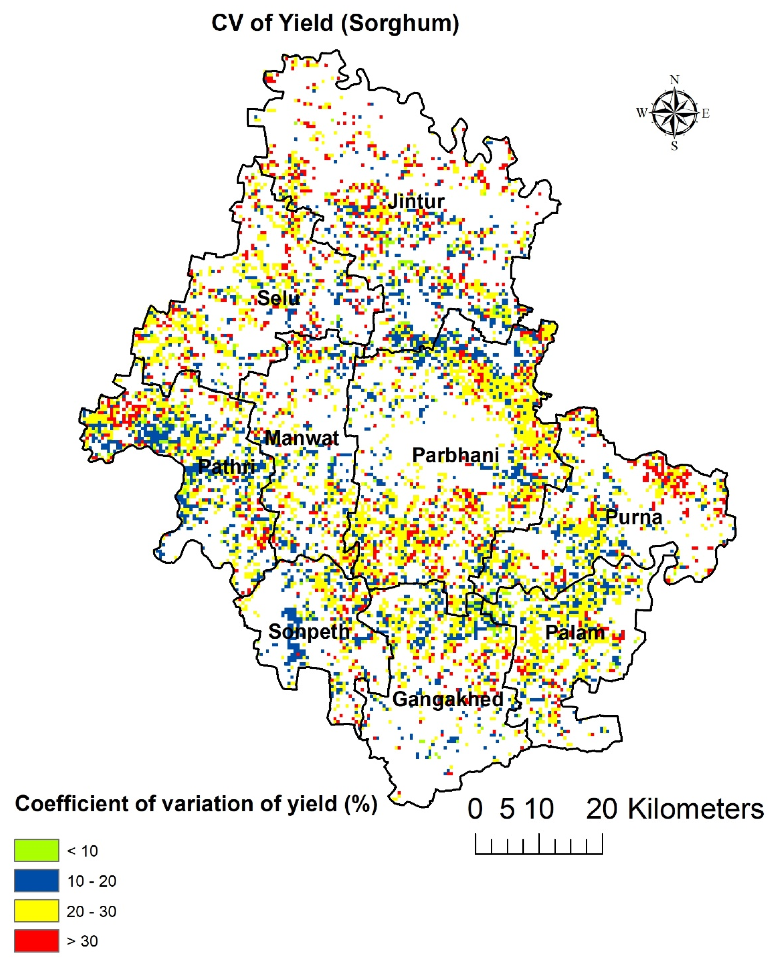
3.2. Disaggregated Crop Yield Map

Using the disaggregation criterion, the rabi sorghum and wheat yield maps were generated for the crop pixels for each crop year of the study. For example, Figure 7 shows the rabi sorghum disaggregated yield map. For the disaggregation, the district production statistics for 2010–2011 were used, and the EVI was integrated at pixels for the period between 3-January-2011 and 30-January-2011. The pixel level yield generated varied between 694 and 1447 kg/ha for the year 2010–2011, and the EVI was integrated at pixels for the period between 1-January-2011 and 2-February-2011. The pixel level wheat yield generated by disaggregation varied between 900 and 2400 kg/ha for the year 2010–2011. To validate the disaggregation methodology and analyse the extent of error, the disaggregated pixel level yield values were aggregated to the sub-district (tehsil/taluk) level and then compared with the values reported by the State Department of Agriculture (SDA) at the sub-district (tehsil/taluk) level. The comparison of estimated and reported rabi sorghum and wheat yield is shown in Figure 8. In general, there was good correspondence between the two with a correlation coefficient of 0.9 for both crops. The methodology underestimated the sorghum yield in sub-districts (tehsils/taluks) having higher yield values, while it overestimated the yield in sub-districts (tehsils/taluks) with lower yield values.
At the sub-district (tehsil/taluk) level, the error between the estimated and reported sorghum yield varied between −22.0% in the Selu sub-district (tehsil/taluk) to +15.8% in the Pathri sub-district (tehsil/taluk) (Figure 8). Overall, the average root mean square error was 167.87 kg/ha, which is about 15.4% of the average district yield. For wheat, at the sub-district (tehsil/taluk) level, the error between the estimated and reported yield varied between −16.0% in the Selu sub-district (tehsil/taluk) to +9.0% in the Manwat sub-district (tehsil/taluk). Overall, the average root mean square error was 178.9 kg/ha, which is about 10.5% of the average district yield.

4. Discussion

Use of remote sensing data for disaggregating existing crop production statistics to the local scale can be highly useful to agricultural planning and implementation of risk management strategies. The remote sensing-based methods provide quick crop yield estimates (downscaled or in-season) covering a vast geographical area. The in-season estimates can be achieved by minor modifications in the methodology described here. A few minor modifications would make this method a predictor model; possible modifications would be the use of vegetation indices at a crop growth stage where yield-vegetation and crop identification are highly correlated.
High resolution yield surface can add substantial value to risk management and planning process in agriculture. These yield surfaces can also give insight to commodity markets and agricultural input planning.
With the space data revolution and availability of more and more datasets with increased spatial and temporal coverages, the accuracy has been substantially increased while costs have come down significantly. Still, there are challenges in obtaining estimates in the rainy season because of cloud cover.
Use of disaggregated crop yields in insurance schemes: Globally, crop insurance is the preferred option for risk transfer. The demand for improved insurance products is increasing. Several countries now operate insurance schemes at the village level; however; unavailability of crop yield and area statistics at this level remains the key bottleneck in implementing or designing such schemes. In India, governments provide a huge subsidy on crop insurance premiums, and the new crop insurance scheme in India is being implemented with the village as the insurance unit [1,38]. The scheme parameters, like threshold yield and loss assessment, are calculated on an area–yield-based approach. Under the previous yield index insurance schemes, the insurance unit was typically at the sub-district level. In the new scheme, the insurance product design and price is based on historical yield values at the village level. A major challenge in implementing a new scheme at the village level is the absence of historical yield series. So, in order to undertake effective implementation of crop insurance schemes with creditability, there is a need to produce a consistent long time-series of historical crop yield data at the local scale (such as village), which may be useful for fixing indemnity limits, threshold yields, premium rates at the village panchayat, or other equivalent units. This methodology is the first step towards getting a historical time-series of yield at the village level using district-level production data and remote sensing techniques. Figure 9 shows coefficient of variation of sorghum yield from 1999–2000 to 2013–2014.
Limitations of the study: This study presented a simple method for downscaling the district level statistics to the sub-district or village or pixel level using a remote sensing approach. Overall, the average root mean square error was 167.87 kg/ha and 178.9 kg/ha, which is about 15.4% and 10.5% of the average district yield for sorghum and wheat, respectively. The error can be attributed to several sources, such as the accuracy of the generated crop mask/decision tree approach and to the data resolution issues considering prevalent small holding farming in the region. Although, the study also validates the approach with the sub-district level using reported statistics. We understand that the study was done over a small geographic area and lacks the validation with the ground truth measurements of crop yield and area. It is likely that the performance of this approach might not be similar for other crops, especially in the rainy season where the availability of quality remote sensing data is low.

5. Conclusions

The study was undertaken to develop and validate a methodology of disaggregation of district level crop yield statistics at the pixel level (i.e., local scale) using satellite remote sensing images. The study procured and pre-processed 500 m MODIS EVI times-series images for 2000–2001 to 2013–2014 crop years for the Parbhani district of Maharashtra State in India. The Savitzky–Golay based filtering technique was adopted in this study for the removal of residual noise in EVI time-series images. A hierarchical decision rule-based image classification technique was adopted for identification and mapping of crop pixels of interest. In the absence of specific ground-truth, the crop growth profile derived phenology events were the basis for fixing the rules during classification.
A simple method was developed and applied for disaggregation of crop district production statistics over crop pixels by using the ratio of EVI of pixel to total EVI of the crop pixels in that district corresponding to the growth phase of crops. It resulted in the generation of crop yield maps at the 500 m resolution pixel (grid) level. The methodology was repeated for all the 14 years to generate time-series of crop yield map. In general, there was good correspondence between disaggregated crop yield and tehsil crop yields with a correlation coefficient of 0.9 for rabi crops in Parbhani (wheat and sorghum). At the sub-district (tehsil/taluk) level, the error between estimated and reported sorghum yield varied between −22.0% in the Selu sub-district (tehsil/taluk) to +15.8% in the Pathri sub-district (tehsil/taluk), and for wheat, −16.0% in the Selu sub-district (tehsil/taluk) to +9.0% in the Manwat sub-district (tehsil/taluk). Overall, the average root mean square error was 178.9 kg/ha, which is about 10.5% of the average district wheat yield. The local scale yield estimates are of immense use in agricultural planning and implementation of risk management strategies. Future research should be targeted at improving these estimates in the rainy season where cloudy conditions pose challenges.

Author Contributions

P.B.S.; V.K.S. and P.K.A. designed the research, V.K.S. and P.B.S. developed methodology and software and analysed the results; V.K.S. and P.B.S. wrote the first draft of the article, which was improved with substantial input from P.K.A. All authors have read and agreed to the published version of the manuscript.

Funding

This research was funded by CGIAR Fund Donors and through bilateral funding agreements.

Acknowledgments

This work was implemented as part of the CGIAR Research Program on Climate Change, Agriculture, and Food Security (CCAFS), which is carried out with support from the CGIAR Trust Fund and through bilateral funding agreements. For details, please visit https://ccafs.cgiar.org/donors. The views expressed in this document cannot be taken to reflect the official opinions of these organizations.

Conflicts of Interest

The authors declare no conflict of interest.

References

  1. Aggarwal, P.K.; Chand, R.; Bhutani, A.; Kumar, V.; Goel, S.K.; Rao, K.N.; Poddar, M.K.; Sud, U.C.; Krishna Murthy, Y.V.N.; Ray, S.S.; et al. Report of the Task Force on Enhancing Technology Use in Agriculture Insurance; CMFRI: Kochi, India, 2016. [Google Scholar]
  2. Gangopadhyay, P.K.; Khatri-Chhetri, A.; Shirsath, P.B.; Aggarwal, P.K. Spatial targeting of ICT-based weather and agro-advisory services for climate risk management in agriculture. Clim. Chang. 2019, 154, 242–256. [Google Scholar] [CrossRef] [Green Version]
  3. Yeh, H.; Lee, C.; Hsu, K.; Chang, P. GIS for the assesment of the groundwater recharge potential zone. Environ. Geol. 2009, 58, 185–195. [Google Scholar] [CrossRef]
  4. Shelia, V.; Hansen, J.; Sharda, V.; Porter, C.; Aggarwal, P.; Wilkerson, C.J.; Hoogenboom, G. A multi-scale and multi-model gridded framework for forecasting crop production, risk analysis, and climate change impact studies. Environ. Model. Softw. 2019, 115, 144–154. [Google Scholar] [CrossRef]
  5. Gyawali, D.R.; Shirsath, P.B.; Kanel, D.; Burja, K.; Arun, K.C.; Aggarwal, P.K.; Hansen, J.W.; Rose, A. Inseason Crop Yield Forecasting for Early Warning Planning of Food Security Using Ccafs Regional Agricultural Forecasting Toolbox (Craft) in Nepal; CGIAR Research Program on Climate Change, Agriculture and Food Security (CCAFS): Wageningen, The Netherlands, 2018. [Google Scholar]
  6. Cantelaube, P.; Terres, J.M. Seasonal weather forecasts for crop yield modelling in Europe. Tellus A Dyn. Meteorol. Oceanogr. 2005, 57, 476–487. [Google Scholar] [CrossRef]
  7. Motha, R.P. Agricultural Drought: USDA Perspectives; Drought Mitigation Center Faculty Publications: Reston, Virginia, USA, 2011. [Google Scholar]
  8. Aggarwal, P.K.; Banerjee, B.; Daryaei, M.G.; Bhatia, A.; Bala, A.; Rani, S.; Chander, S.; Pathak, H.; Kalra, N. InfoCrop: A dynamic simulation model for the assessment of crop yields, losses due to pests, and environmental impact of agro-ecosystems in tropical environments. II. Performance of the model. Agric. Syst. 2006, 89, 47–67. [Google Scholar] [CrossRef]
  9. Aggarwal, P.K.; Kalra, N.; Chander, S.; Pathak, H. InfoCrop: A dynamic simulation model for the assessment of crop yields, losses due to pests, and environmental impact of agro-ecosystems in tropical environments. I. Model description. Agric. Syst. 2006, 89, 1–25. [Google Scholar] [CrossRef]
  10. Byjesh, K.; Kumar, S.N.; Aggarwal, P.K. Simulating impacts, potential adaptation and vulnerability of maize to climate change in India. Mitig. Adapt. Strateg. Glob. Chang. 2010, 15, 413–431. [Google Scholar] [CrossRef]
  11. Kumar, S.N.; Aggarwal, P.K.; Saxena, R.; Rani, S.; Jain, S.; Chauhan, N. An Assessment of Regional Vulnerability of Rice to Climate Change in India. Climatic Chang. 2013, 118, 683–699. [Google Scholar]
  12. Timsina, J.; Godwin, D.; Humphreys, E.; Kukal, S.S.; Smith, D. Evaluation of options for increasing yield and water productivity of wheat in Punjab, India using the DSSAT-CSM-CERES-Wheat model. Agric. Water Manag. 2008, 95, 1099–1110. [Google Scholar] [CrossRef]
  13. Subash, N.; Ram Mohan, H.S. Evaluation of the impact of climatic trends and variability in rice-wheat system productivity using Cropping System Model DSSAT over the Indo-Gangetic Plains of India. Agric. For. Meteorol. 2012, 164, 71–81. [Google Scholar] [CrossRef]
  14. Mohanty, M.; Probert, M.E.; Reddy, K.S.; Dalal, R.C.; Mishra, A.K.; Subba Rao, A.; Singh, M.; Menzies, N.W. Simulating soybean-wheat cropping system: APSIM model parameterization and validation. Agric. Ecosyst. Environ. 2012, 152, 68–78. [Google Scholar] [CrossRef]
  15. Singh, P.K.; Singh, K.K.; Bhan, S.C.; Baxla, A.K.; Singh, S.; Rathore, L.S.; Gupta, A. Impact of projected climate change on rice (Oryza sativa L.) yield using CERES-rice model in different agroclimatic zones of India. Curr. Sci. 2017, 112, 108–115. [Google Scholar] [CrossRef]
  16. Jones, J.; Hoogenboom, G.; Porter, C.; Boote, K.; Batchelor, W.; Hunt, L.; Wilkens, P.; Singh, U.; Gijsman, A.; Ritchie, J. The DSSAT cropping system model. Eur. J. Agron. 2003, 18, 235–265. [Google Scholar] [CrossRef]
  17. Singh, A.K.; Tripathy, R.; Chopra, U.K. Evaluation of CERES-Wheat and CropSyst models for water-nitrogen interactions in wheat crop. Agric. Water Manag. 2008, 95, 776–786. [Google Scholar] [CrossRef]
  18. Sudhir-Yadav, S.; Li, T.; Humphreys, E.; Gill, G.; Kukal, S.S. Evaluation and application of ORYZA2000 for irrigation scheduling of puddled transplanted rice in north west India. Field Crops Res. 2011, 122, 104–117. [Google Scholar] [CrossRef]
  19. Dadhwal, V.K.; Sehgal, V.K.; Singh, R.P.; Rajak, D.R. Wheat yield modelling using satellite remote sensing with weather data: Recent Indian experience. Mausam 2003, 54, 253–262. [Google Scholar]
  20. Becker-Reshef, I.; Justice, C.; Sullivan, M.; Vermote, E.; Tucker, C.; Anyamba, A.; Small, J.; Pak, E.; Masuoka, E.; Schmaltz, J.; et al. Monitoring Global Croplands with Coarse Resolution Earth Observations: The Global Agriculture Monitoring (GLAM) Project. Remote Sens. 2010, 2, 1589–1609. [Google Scholar] [CrossRef] [Green Version]
  21. Lobell, D.B.; Burke, M.B. On the use of statistical models to predict crop yield responses to climate change. Agric. For. Meteorol. 2010, 150, 1143–1152. [Google Scholar] [CrossRef]
  22. Burke, M.; Lobell, D.B. Satellite-based assessment of yield variation and its determinants in smallholder African systems. Proc. Natl. Acad. Sci. USA 2017, 114, 2189–2194. [Google Scholar] [CrossRef] [Green Version]
  23. Jin, X.; Kumar, L.; Li, Z.; Feng, H.; Xu, X.; Yang, G.; Wang, J. A review of data assimilation of remote sensing and crop models. Eur. J. Agron. 2018, 92, 141–152. [Google Scholar] [CrossRef]
  24. Weiss, M.; Jacob, F.; Duveiller, G. Remote sensing for agricultural applications: A meta-review. Remote Sens. Environ. 2020, 236, 111402. [Google Scholar] [CrossRef]
  25. Lobell, D.B.; Azzari, G. Satellite detection of rising maize yield heterogeneity in the U.S. Midwest. Environ. Res. Lett. 2017, 12, 014014. [Google Scholar] [CrossRef]
  26. Azzari, G.; Jain, M.; Lobell, D.B. Towards fine resolution global maps of crop yields: Testing multiple methods and satellites in three countries. Remote Sens. Environ. 2017, 202, 129–141. [Google Scholar] [CrossRef]
  27. Lobell, D.B.; Thau, D.; Seifert, C.; Engle, E.; Little, B. A scalable satellite-based crop yield mapper. Remote Sens. Environ. 2015, 164, 324–333. [Google Scholar] [CrossRef]
  28. Chakrabarti, S.; Bongiovanni, T.; Judge, J.; Zotarelli, L.; Bayer, C. Assimilation of SMOS Soil Moisture for Quantifying Drought Impacts on Crop Yield in Agricultural Regions. IEEE J. Sel. Top. Appl. Earth Obs. Remote Sens. 2014, 7, 3867–3879. [Google Scholar] [CrossRef]
  29. Ines, A.V.M.; Das, N.N.; Hansen, J.W.; Njoku, E.G. Assimilation of remotely sensed soil moisture and vegetation with a crop simulation model for maize yield prediction. Remote Sens. Environ. 2013, 138, 149–164. [Google Scholar] [CrossRef] [Green Version]
  30. Nearing, G.S.; Crow, W.T.; Thorp, K.R.; Moran, M.S.; Reichle, R.H.; Gupta, H.V. Assimilating remote sensing observations of leaf area index and soil moisture for wheat yield estimates: An observing system simulation experiment. Water Resour. Res. 2012, 48. [Google Scholar] [CrossRef] [Green Version]
  31. Gao, X.; Huete, A.R.; Ni, W.; Miura, T. Optical–Biophysical Relationships of Vegetation Spectra without Background Contamination. Remote Sens. Environ. 2000, 74, 609–620. [Google Scholar] [CrossRef]
  32. Chen, X.; Vierling, L.; Rowell, E.; DeFelice, T. Using lidar and effective LAI data to evaluate IKONOS and Landsat 7 ETM+ vegetation cover estimates in a ponderosa pine forest. Remote Sens. Environ. 2004, 91, 14–26. [Google Scholar] [CrossRef]
  33. Lovell, J.L.; Graetz, R.D. Filtering Pathfinder AVHRR Land NDVI data for Australia. Int. J. Remote Sens. 2001, 22, 2649–2654. [Google Scholar] [CrossRef]
  34. Cihlar, J.; Ly, H.; Li, Z.; Chen, J.; Pokrant, H.; Huang, F. Multitemporal, multichannel AVHRR data sets for land biosphere studies—Artifacts and corrections. Remote Sens. Environ. 1997, 60, 35–57. [Google Scholar] [CrossRef]
  35. Gutman, G.G. Vegetation indices from AVHRR: An update and future prospects. Remote Sens. Environ. 1991, 35, 121–136. [Google Scholar] [CrossRef]
  36. Casley, D.; Kumar, K. The Collection, Analysis, and Use of-Monitoring and Evaluation Data a World Bank Publication; World Bank: Washington, DC, USA, 1988. [Google Scholar]
  37. Poza, M.; Bhagia, N.; Patel, J.H.; Dutta, S.; Dadhwal, V.K. National Wheat Acreage Estimation for 1995-96 Using Multi-Date IRS-1C WiFS Data. J. Indian Soc. Remote Sens. 1996, 24, 243–254. [Google Scholar] [CrossRef]
  38. Gulati, A.; Tewary, P.; Hussain, S. Crop Insurance in India: Key Issues and Way Forward; Working Paper No. 352; Indian Council for Research on International Economic Relations: New Delhi, India, 2018. [Google Scholar]
Figure 1. Map of sub-districts (tehsils/taluks) of Parbhani, Maharashtra (background image depicts the Enhanced Vegetation Index (EVI)).
Agriculture 10 00058 g001
Figure 2. The overall methodology flowchart showing the steps followed in this study. The steps on the left describe data pre-processing, the middle column describes crop mapping, and the column on the right describes yield downscaling.
Agriculture 10 00058 g002
Figure 3. The raw and filtered EVI profile of pixels over 2000–2001 kharif and rabi crops. The inset shows zoomed up raw and filtered EVI profiles for the 2004–2005 crop season.
Agriculture 10 00058 g003
Figure 4. (a) The MODIS land cover map of the study region with land cover classes and (b) cropland mask of the study region.
Agriculture 10 00058 g004
Figure 5. The crop area map of the Parbhani district using hierarchical decision rule-based classification of time-series of an EVI profile.
Agriculture 10 00058 g005
Figure 6. Comparison remote sensing estimated (RS) wheat crop (a) and sorghum (b) area with those reported by the State Department of Agriculture (SDA) for the sub-districts (tehsils/taluks) of Parbhani.
Agriculture 10 00058 g006
Figure 7. The disaggregated wheat (a) and sorghum (b) yield map for the year 2010–2011.
Agriculture 10 00058 g007
Figure 8. Comparison of disaggregated yield (RS) and reported yield (SDA) at the sub-district (tehsil/taluk) level, and the per cent error for the winter (rabi) season of 2010–2011.
Agriculture 10 00058 g008
Figure 9. Coefficient of variation of sorghum yield from 1999–2000 to 2013–2014.
Agriculture 10 00058 g009

