Abstract
Particle filter has received increasing attention in data assimilation for estimating model states and parameters in cases of non-linear and non-Gaussian dynamic processes. Various modifications of the original particle filter have been suggested in the literature, including integrating particle filter with Markov Chain Monte Carlo (PF-MCMC) and, later, using genetic algorithm evolutionary operators as part of the state updating process. In this work, a modified genetic-based PF-MCMC approach for estimating the states and parameters simultaneously and without assuming Gaussian distribution for priors is presented. The method was tested on two simulation examples on the basis of the crop model AquaCrop-OS. In the first example, the method was compared to a PF-MCMC method in which states and parameters are updated sequentially and genetic operators are used only for state adjustments. The influence of ensemble size, measurement noise, and mutation and crossover parameters were also investigated. Accurate and stable estimations of the model states were obtained in all cases. Parameter estimation was more challenging than state estimation and not all parameters converged to their true value, especially when the parameter value had little influence on the measured variables. Overall, the proposed method showed more accurate and consistent parameter estimation than the PF-MCMC with sequential estimation, which showed highly conservative behavior. The superiority of the proposed method was more pronounced when the ensemble included a large number of particles and the measurement noise was low.
1. Introduction
Crop development and geophysical and hydrological processes can be represented by simulation models, which are used to predict the process state. One of the usages of such dynamic models is the development of decision support systems (DSS). Since an imperfect model may lead to incorrect decisions, model imperfectness is often cited as one of the main drawbacks of model-based DSS. The crop-soil-atmosphere model AquaCrop developed by the Food and Agriculture Organization (FAO, Rome, Italy) [1,2] is one of the models commonly used in DSS studies that focus on irrigation management [3,4,5,6], mainly due to its relative simplicity, robustness, and reasonable accuracy for a wide range of crops. However, very little literature is available on data assimilation in AquaCrop, especially with Bayesian approaches (e.g., particle filter) [7]. The scope of the present study was to develop a data assimilation framework for crop-soil-atmosphere models on the basis of particle filter, and analyze its performance with AquaCrop.
Data assimilation methods were originally developed for state estimation, but various studies have extended them to the estimation of the model parameters as well. One of the commonly used methods is the ensemble Kalman filter (EnKF) [8,9], which uses the Monte Carlo approach to estimate the state covariance on the basis of the ensemble covariance. This covariance is used as state covariance within the equations of Kalman filter [10]. However, EnKF suffers from several limitations that might result in sub-optimal performance, such as non-Gaussian state distribution and physical violation update. Therefore, some modifications might be applied to EnKF to alleviate these problems, such as covariance inflation, relaxation, and estimation modification [11,12,13,14,15,16]. However, these methods are case-dependent and involve user-defined tuning parameters that strongly influence the assimilation performance. Hence, in the literature, EnKF-based methods are increasingly replaced by approaches based on particle filter (PF) [17,18,19]. Generally speaking, PF relies less heavily on tuning parameters and uses Bayesian estimations by resampling rather than updates based on correlations that, as noted above, might be spurious when the tuning parameters are not set properly. DeChant and Moradkhani [13] compared the performance of EnKF and PF, showing more robust and effective uncertainty reduction by PF-based approaches than by EnKF-based ones in terms of state distribution and parameter estimations. More recently, Chen and Cournède [20] compared the performance of two Kalman filter (KF)-based approaches (unscented Kalman filter (UKF) and EnKF) and a PF-based approach with the log-normal allocation and senescence model for sugar beet. Their results showed that KF-based approaches suffered from the significant nonlinearity of the model, in contrast to PF-based methods.
In particle filters, estimation is based on running in parallel an ensemble of models (so-called particles) and weighting them on the basis of the measurements. One limitation of PF is particle degeneracy, as some particles become associated with negligible weights. This might cause involving unimportant particles in the assimilation process, resulting in a non-representative ensemble and low computational efficiency. Several methods have been suggested to alleviate this problem. Moradkhani et al. [21], who worked with a hydrological model, suggested perturbing the parameters using Gaussian noise after resampling the state. The Gaussian noise was calculated on the basis of the particle ensemble. Similar methods have been used in other studies related to land surface models and soil hydrology [22,23]. Recently, Berg et al. [19] suggested resampling particles by stochastic universal resampling, in which some particles are discarded and new particles are generated using Gaussian distribution to maintain the ensemble size. The Gaussian distribution parameters were calculated on the basis of a weighted augmented state ensemble (i.e., ensemble that consists of state and parameters). However, in this approach the new particles might be worse than the original ones since the sampling from the Gaussian distribution is random and not based on deductive sampling. Another limitation is that the method involves a tuning parameter that might affect the method performance, and, in some cases, numerical problems might arise when calculating the eigenvalues of the ensemble covariance matrix, which is needed for calculating the tuning parameters, especially when the state vector is large [19].
Another method suggested to reduce weight degeneracy is the combination of PF with Monte Carlo Markov Chain (MCMC) [24,25]. Integrating MCMC with PF can help replacing low probability particles with particles that have higher probabilities to survive. However, this method by itself only determines whether to accept or reject particles, without suggesting alternative (better) particle candidates. So-called intelligent search and optimization methods categorized as metaheuristic algorithms (MAs) have also been used to mitigate the degeneracy problem. Among these, combining genetic algorithm (GA) with PF has received increasing attention in recent years. However, due to the high computational cost, the literature suggests incorporating only the evolutionary concept of the GA instead of formulating the PF into a full GA optimization problem. For instance, Kwok et al. [26] suggested an evolutionary PF in which some prior particles were generated using the crossover operator only, i.e., new children particles were generated from couples of parent particles. Yin and Zhu [17] used crossover and mutation within PF and concluded that utilizing GA operators improves PF estimations. However, the generated particles should be selected properly so that the shuffled particles do not move outside of the posterior distribution. Abbaszadeh et al. [18] suggested incorporating MCMC together with GA evolutionary operators (crossover and mutations) in PF in order to form what they termed an ‘evolutionary particle filter MCMC (EPFM)’, which assured proper particle selection and avoided filter degeneracy. At each assimilation step, the states were crossed-over and mutated, and state selection was performed by MCMC. Finally, on the basis of the selected states, the parameters were updated using MCMC. However, this process of estimating sequentially the states and then the parameters (using the previously obtained states) might lead to sub-optimality, as both states and parameters should be evaluated simultaneously. In addition, the parameters were determined using only MCMC without exploiting the potential of using GA evolutionary operators at that step.
In the present work, a modified formulation of EPFM, referred to below as genetic-based PF combined with MCMC (GPFM), is introduced. This formulation enables simultaneous estimation of the states and parameters and exploits genetic operations and MCMC for both state and parameter estimations. This method improves the existing methods (specifically [18]) by applying (at each time step) simultaneous (optimal) rather than sequential (sub-optimal) state and parameter estimation. The GPFM is illustrated on two synthetic examples using a slightly modified version of the crop model AquaCropOS [27], which is an open-source version of the AquaCrop model. In the first example, GPFM is compared with the method described in [18].
2. Materials and Methods
2.1. Background
Nonlinear dynamic systems are often described by the following finite difference equations:
where () denotes the model, denotes the measurements operator, denotes the state vector at time , is the (uncertain) forcing data, is the vector of model parameters, and is the vector of measurements. and are the process and measurements noise, respectively, which are assumed to be white noises with zero mean and covariance and , respectively. In addition, they are assumed to be independent. On the basis of Bayesian estimation, given a measurement at time , the posterior distribution of the state at time is as follows:
where is the probability of the observed measurement given the estimated state at time , is the prior distribution of the state, and is a normalization factor. The analytical solution of Equation (3) cannot be obtained due to the non-linearity of the process and the multi-dimensionality of the problem. Hence, the posterior distribution is often approximated using an ensemble of models. In PF terminology, the states and parameters associated with each model form a particle. Each particle is associated with a weight, which quantifies its likelihood on the basis of the observations. Both particles and weights evolve dynamically. In [18], each particle is divided conceptually of two components that correspond to the model states and parameters, respectively. At each assimilation step, these two components are updated sequentially as follows (Figure 1 in [18]):
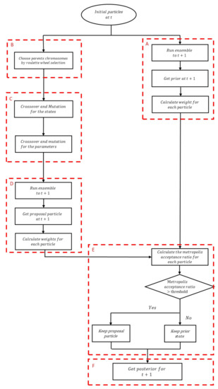
Figure 1.
Overall genetic-based particle filter combined with Monte Carlo Markov Chain (GPFM) framework, which consists of six stages (labeled (A–F)).
- State adjustment
- The current states are propagated to time t + 1 using the corresponding models, yielding so-called prior states.
- The weights corresponding to these prior states are calculated.
- New states are generated by applying cross-over and mutations to the current states.
- The new states are propagated to time t + 1 using the corresponding models, yielding so-called proposal prior states.
- The weights corresponding to these proposal prior states are calculated.
- The MCMC Metropolis Hastings ratio of the proposal prior states to prior states is used to determine which particle is accepted.
- The parameters are adjusted using MCMC Metropolis Hastings [25]. Conceptually, this consists of generating proposal parameters by adding random noise to the current parameters and calculating MCMC Metropolis Hastings ratio to accept or reject the proposal parameters.
2.2. Proposed Approach
The flowchart of the present procedure is shown in Figure 1. Whereas in the procedure developed in [18], the states and parameters are updated in a serial fashion, in the present procedure, the 2 halves of the particles (states and parameters) are adjusted simultaneously. More specifically, crossover and mutation operations are applied to each half particle (Figure 1C). Both operators are applied over particles previously selected by Roulette wheel selection (Figure 1B). The basic idea behind the Roulette wheel selection is the same as the roulette in casino. First, a fitness value is associated to each candidate particle. Second, the fitness values are normalized so that their sum is 1. Third, the fitness values are arranged in a vector in random order. Fourth, a random number between 0 and 1 is generated from a uniform distribution and chosen particle is the particle that the random number points to. This way, candidates with high fitness values are more likely to be selected. Step 4 is repeated until the appropriate number of particles have been obtained.
Numerous crossover methods have been proposed in literature (e.g., arithmetic and discrete crossovers) [28,29]. Arithmetic crossover is a widely used method in the context of evolutionary PF [17,30], and is adopted here for simplicity. Other crossover operations could be used in a similar fashion. For the states, the crossover operation corresponds to
where and denote the states of the parent particles with indices and , respectively, and is a user-defined crossover parameter for state.
The parameters are adjusted in a similar fashion:
where is a user-defined crossover parameter for parameters.
In addition to crossover, mutation is performed to increase the diversity of the particles, i.e., increase the chances of covering a wider span of the parameters and state space. More specifically, one gene of the state vector and one gene of the parameter vector (both chosen randomly) are mutated:
where the and subscripts denote the number of the gene within the particle, and represent random Gaussian noises, and and denote the variances of state and parameters. and could be chosen according to the gene within the particle, e.g., large number could be chosen as the variance of the gene is small and vice versa. After executing crossover and mutation for states and parameters, the new crossed-over and mutated state, together with crossed-over and mutated parameters, are propagated to obtain proposal state:
where and are the state and parameters obtained by crossover and mutation, and is the proposal state. The combination of the proposal state with the corresponding parameters form the proposal particle (Figure 1D).
The probability distribution function (PDF) of the proposed joint state parameters is approximated as (without dividing with the probability of the measurements):
where because the parameters are not dynamic. is calculated on the basis of the likelihood as follows:
where is the measurements covariance.
Each proposal particle is examined by MCMC Metropolis Hastings in order to determine whether to accept or reject it (Figure 1E). Basically, the proposal particles are compared with prior particles which consist of the parameters before crossover and mutation and state which is obtained by running the simulation model with these parameters (Figure 1A).
In order for one to calculate the prior probabilities, and , an assumption is often made about the distribution of the priors of the parameters and state (e.g., Gaussian distribution). Then, the PDF of the proposal and priors are compared via the Metropolis acceptance ratio:
where and are, respectively, the prior state and parameters for particle at time . To avoid assuming Gaussian distribution of the state and parameters and to exploit the ability of PF to deal with non-Gaussian distributions, we assume heuristically that the distributions of the proposal state and parameters are equal to the prior distributions of the state and parameters. In order to minimize the violation of this assumption, in the examples below, we impose that the changes of the state and parameters due to crossover and mutation remain small. The Metropolis acceptance ratio is then approximated as follows:
In other words, if the Metropolis acceptance ratio is above a specified threshold, then the proposal particle as accepted, otherwise it is rejected. This acceptance or rejection process ensures that, at each assimilation step, particles with higher probability to represent the posterior are accepted, resulting in a more reliable posterior distribution (Figure 1F). It is worth mentioning that the weights of the particles are initialized as 1/N in each assimilation step, since otherwise small weights are obtained de facto after a large number of assimilation steps. A resampling step can be applied after the assimilation step. In this step, particles with high weights are replicated and those with low weights are dropped to obtain more representative particles. However, in the present study, since the roulette wheel selection and the MCMC are based on the weights of the particles, only particles with high weights (i.e., highly representative particles) are selected, and therefore such a resampling step was found to be not essential.
It is worth mentioning that Equations (7), (8), and (10) were not used in previous works and form the core of GPFM, using GA operators for both states and parameters estimations.
3. Examples
The method described above was tested over two synthetic examples. In both cases, the (optional) resampling step was found to have only negligible impact on the results (details not shown), and the results presented below were obtained without implementing this step. This lack of need for resampling can be explained by the fact that the roulette wheel selection (used in Step B in Figure 1) led to discarding most particles with small weights while keeping the particles with high weights. Since most of the resulting particles were characterized by high weights, subsequent application of resampling eliminated very few particles and hence had only marginal influence.
The examples were based on a slightly modified version of the crop model AquaCrop-OS v5.0a [27], an open-source version of the model AquaCrop. AquaCrop is daily time-step water-driven simulation model that simulates crop development and soil water dynamics. A full description of this model is beyond the scope of this paper and can be found in [1], as well as in the documentation available on the FAO AquaCrop website. Only some key elements pertinent to the present work are briefly described here.
Crop development involves four main processes: canopy growth and decline, transpiration, biomass accumulation, and partitioning of biomass into yield. These processes are influenced by water availability on the root zone, which is obtained by simulating water flow within the user-defined soil layers.
- 1.
- Simulation of canopy growth and decline:
Canopy development is split into three periods:
- Exponential growth as long as
- Exponential decay, when and until senescence
- Canopy decline, after the onset of senescence:
In these equations, is initial canopy cover; and are the canopy growth and decline coefficients, respectively; is the maximum canopy cover; and denotes day from planting/sowing.
- 2.
- Estimation of crop transpirationwhere is a crop-dependent coefficient used to express the impact of stress, is the canopy size (adjusted for micro-advective effects), and is the reference evapotranspiration.
- 3.
- Simulation of above-ground biomass:where is the above-ground biomass, is the water productivity, and expresses the influence of temperature stress on biomass accumulation.
- 4.
- Partitioning of biomass into yield :where is the harvest index at .
The soil is modeled as a series of layers with user-specified thickness, texture, and hydraulic properties. The water content in each layer is computed via a simple water balance equation:
where denotes the difference in the water amount in layer , denotes the water flowing into layer from the previous layer (irrigation and rain in top layer), and denotes the sum of the water flowing from layer into the next layer and the water removed by the roots (and evaporation in top layer). These terms depend on soil-dependent parameters (among them, water content at field capacity and saturation and , respectively, and hydraulic conductivity at saturation, ) as well as on crop parameters (e.g., maximum flux extractable by roots). The impact of water availability on crop development is expressed through relationships that involve water content in the root zone and various crop-specific parameters.
For the sake of the present work, the main observation of the above description is that canopy cover (CC) is modeled via algebraic equations (i.e., hard-coded relationship between CC and time). In other words, canopy cover is not a state variable in the model, and data assimilation is not possible. This is rather regretful, as canopy cover (or leaf area index) is currently the only canopy measurement that can be performed relatively easily in the field [31,32,33]. Therefore, in the present study, we re-coded canopy cover development with the equivalent difference equations:
Equation (16) was replaced by
Equation (17) was replaced by
and Equation (18) was replaced by
It can be easily verified that if data assimilation is not performed (i.e., CC and the parameters are not adjusted), Equations (16)–(19) and (23)–(25) are strictly equivalent. The advantage of the new formulation is that CC is now described by dynamic equations, and thus CC is a state variable to which data assimilation can be applied.
3.1. Case Study #1
A hypothetic cotton crop in Greece was used as first case study. The soil profile consisted of three layers of sandy loam, clay loam, and clay, with respective thicknesses of 0.4, 0.3, and 1.3 m. The soil water content was assumed to be at field capacity on the sowing date (1 May 2015). The simulation was run with climatic data (temperature, precipitation, and potential evapotranspiration ) obtained from the Democritus University of Thrace meteorological station in northern Greece. Irrigation was applied according to irrigation schedule in Table 1.

Table 1.
Irrigation schedule in case study #1.
Two models that differed in terms of the crop parameters listed in Table 2 were used—a ‘true’ model and a ‘biased’ model that was used as starting point for the assimilation process. All other parameters were as listed in [4].
Table 2.
Crop parameters of the true and biased models (case study #1).
When testing GPFM, each of the parameters listed in Table 2 was estimated at each time step (daily), while all other parameters were kept constant. These parameters were chosen as they influence the calculations of soil water content, canopy cover, and/or biomass and, ultimately, yield. The virtual measurements consisted of canopy cover and water content at 20, 40, 60, 80, and 100 cm, which were generated using the true model. The state vector consisted of the water content at 5 cm incremental depths along the 200 cm depth soil profile and the canopy cover. This state vector (size 21) was updated at each assimilation step. During the assimilation process, the following lower and upper boundaries were imposed to avoid unrealistic values:
where and are the true and biased parameters, respectively. Estimations that were not inside the boundaries were set to the corresponding boundary values. These boundaries were applied in the second case study as well.
As detailed below, several tests were conducted to analyze the influence of various tuning parameters: the parameters controlling state and parameters crossover (Equations (5)–(8) and mutation (Equations (9) and (10)), measurement noise, and ensemble size. GPFM was compared to the EPFM method of [19], in which the state and parameters are adjusted sequentially in two separate steps.
3.2. Case Study #2
The second case study was conducted with a hypothetic quinoa crop in Israel. The soil profile consisted of three 0.2 m depth layers of sandy clay soils. The quinoa sowing date was 1 February 2017, and the simulation was performed from this date until 1 August 2017. The soil water content was assumed to be at field capacity on the sowing date. The simulation was run with climatic data (temperature, precipitation, and potential evapotranspiration ) obtained from the Technion meteorological station and the Ein HaHoresh station of the Israel Meteorological Service, Bet-Dagan, Israel. Interpolations were conducted to fill in a few missing records. Irrigation was applied weekly from 1 March until 24 July in 50 mm amounts. As in case study #1, ‘true’ and ‘biased’ models were used, but here the models differed in terms of both crop and soil parameters, as detailed in Table 3. Crop parameters not listed in Table 3 were kept at the default values provided in the quinoa model included in the AquaCrop package.
Table 3.
Soil and crop parameters of the true and biased models (case study #2).
Each of the parameters listed in Table 3 were estimated by assimilation process at each time step (daily), while all other parameters were kept to their nominal value [1]. The virtual measurements consisted of canopy cover and water content at 5, 15, and 25 cm, which were generated using the true model with 5% standard deviation white Gaussian noise.
The crossover factor for state () and parameters () were set to 0.05 and 0, respectively (i.e., no crossover for the parameters). For mutation ( and ), 5% standard deviation was chosen. In each assimilation step, the water content at 2 cm increments along the 60 cm depth soil profile and the canopy cover were updated (the state size was 31). The ensemble size used in this case study was 500, and the particles were initialized with the biased parameter values perturbated with 5% standard deviation (STD) white Gaussian noise. The standard deviation of the measurement noise was 0.05 and 0.005 for water content and canopy cover measurement, respectively.
4. Results and Discussions
4.1. Case Study #1
4.1.1. Accuracy of Parameters Estimations
The discrepancies between estimations (at the current time step) or predictions (of the future time steps) and measurements can be reduced in two ways: by improving the parameter estimates and by adjusting the states. According to Equations (5)–(10), the extent of the adjustments of the parameters and states are controlled by and , and and , respectively. Intuitively, relatively larger values of and are expected to force the filter to reduce the modeling errors by improving the parameter estimates, while relatively larger values of and should enable the filter to reduce the modeling error mostly by state adjustments, while not necessarily promoting convergence of the parameters toward their true value. To validate this intuitive reasoning, we investigated three combinations of these two parameters, corresponding to stronger adjustments of the parameters, stronger adjustments of the states, and similar adjustments of parameters and state. This analysis was conducted with an ensemble consisting of 1500 particles. The results obtained with these three combinations are shown in Figure 2 and Figure 3 (the tuning parameters used in each of the combinations A1–A3 appear in Table 4). These Figures show the average value of the relevant state/parameters calculated over the whole ensemble. It can be observed in Figure 2 that data assimilation improved CC estimations drastically, and almost perfect estimations were achieved with all three parameter combinations. Similar results were observed for estimation of soil water content profile in all three cases (not shown). As expected, these improvements led to overall improvement of yield estimates. Whereas without data assimilation the predicted yield was 4.92 , data assimilation led to yield estimates ranging from 4.31 to 4.33 t/ha, significantly closer to the true value (4.49 ).
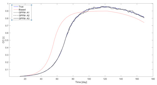
Figure 2.
Canopy cover for the true (bold line) and biased (solid line) cases and for GPFM using various tuning parameters (broken lines) in case study #1.

Figure 3.
Absolute relative error (relative to the true values) for the crop parameter estimations with GPFM using various tuning parameters in case study #1. The error of the biased model (without data assimilation) is also shown for comparison (solid line). Frame (a) shows the error for the canopy growth coefficient; Frame (b) shows the error for the maximum root water extraction at the bottom of the root zone; Frame (c) shows the error for the maximum root water extraction at top of the root zone and Frame (d) shows the error for the maximum canopy cover.
Table 4.
Average relative errors in parameter estimation (Equation (27)) for various values of the crossover and mutation parameters.
Improvements in parameter estimations can be seen in Figure 3, which shows the absolute error between the actual and estimated values of the four parameters included in the analysis. As can be seen in Equation (16), the parameter CGC controlled early canopy development, which in turn determined transpiration (water uptake) and biomass accumulation, so that its value influenced all states most strongly. However, it must be noted that CGC did not enter the calculations until CCx was reached (see Equations (18) and (19)), which occurred around day 72, and thus the error in this parameter beyond that date is irrelevant. Until then, data assimilation led to significant improvement in the estimation of this parameter (Figure 3a). As expected, larger values of and compared to and led to faster convergence and greater overall improvement. Data assimilation also led to consistent improvement in the estimation of SxBotQ (maximum root water extraction at top of the root zone) (Figure 3b), with again greater and faster improvements obtained for larger values of and compared to and . It is noteworthy that these two parameters had the largest initial relative errors. For the parameters SxTopQ (maximum root water extraction at the bottom of the root zone) and CCx, the behavior was more erratic. SxTopQ affected the computations mostly during the early stages of crop development, when the rooting depth was still limited. The erratic behavior of CCx could be due the fact that it had direct influence of the canopy cover estimations during part of the growth period. In case of low adjustment of the parameters relative to the state adjustment, the CCx was estimated more accurately (Figure 3d). The overall improvements achieved for all three combinations are summarized in Table 4, which shows the average error (relative to the error of the biased model) in parameter estimate (over the ensemble) averaged over time as follows:
where is the posterior parameter within particle at time , is the length of the growing period, and is the ensemble size.
On the basis of these results that showed better performance when favoring parameter adjustments over state adjustments, we conducted most of the subsequent analyses with such a configuration.
Decreasing the ensemble size was expected to negatively impact the overall performance of the filter, especially since, compared to sequential estimations of the state and parameters, simultaneous estimation enlarged the problem substantially. The results shown in Table 5 show that this was indeed the case. It is noteworthy that for CGC, which, as discussed above, influences the computations strongly but only for a limited period, a significant improvement was obtained even with small ensemble sizes. For less influential parameters such as SxtopQ and SxbotQ, significant improvements were obtained only with large ensemble sizes.
Table 5.
Average errors in parameter estimation (Equation (27)) for various ensemble sizes. The results obtained with evolutionary particle filter Monte Carlo Markov Chain (EPFM) are given in parentheses for comparison.
When comparing the results of GPFM with the results of the EPFM method of Abbaszadeh et al. [17], we can observe that the influence of the ensemble size on the parameters improvements was much stronger and consistent for the present method. With EPFM, a 10-fold increase of the ensemble size only marginally improved the estimations of most parameters. This conservative behavior can be attributed to the fact that the parameter estimation was based on random perturbation rather than mutation and crossover, which are based on roulette wheel selection. As mentioned, roulette wheel selection is most likely to choose the particles with high weights.
This behavior was further observed in a second analysis, in which the state adjustments were favored over parameter adjustment (Table 5, bottom rows). In this case, EPFM did not result in any parameter improvements due to the low adjustment of the parameters. It worth mentioning that in this case GPFM improved CCx estimations significantly.
A final analysis investigated the impact of the measurement noise on the parameter estimations. The ensemble size used in this case study was 1000. Lower measurement noise is equivalent to greater confidence in the measurements, which leads to high likelihoods of the particles, which are close to the measurements (Equation (13)), high weights, high acceptance ratio (Equation (15)), and ultimately stronger adjustments of the parameters and/or states towards the true values. The results shown in Table 6 show that this was indeed the case for GPFM, which showed overall good estimations in low measurement noise. On the other hand, the results obtained with EPFM were only marginally affected by the amplitude of the measurement noise. As with ensemble size, an additional test was conducted under low parameter adjustment relative to the state adjustment. In this case, GPFM estimations remained satisfactory, while EPFM failed to achieve good results (Table 6, bottom rows). It worth mentioning that in this test, CCx became the parameter most significantly improved. This agrees with the results presented above and strengthens the observation that CCx has to be adjusted moderately due to its high influence on the canopy cover.
Table 6.
Average errors in parameter estimation (Equation (27)) for various measurement noise values. The results obtained with EPFM are given in parentheses for comparison.
In summary, the largest improvements were obtained for the estimation of CGC, which influences canopy development strongly and directly and indirectly influences other crop processes. The estimation of CCx was better in cases where the parameters were adjusted moderately, due to its large influence of the measured state. The influence of the parameters SxbotQ and SxtopQ on crop development was much more limited, and the estimated parameters remained close to their original values. These results emphasize the relation between the accuracy of the parameter estimation and their influence of the measured state, as discussed in literature [34,35,36].
Overall, the three factors investigated affected the performance of GPFM as expected. More accurate parameter estimations were obtained with larger ensembles; lower measurement noise; and, when favoring parameters, adjustments over state adjustments. By comparison, these three factors had a much weaker impact on the performance of EPFM. Two factors can explain the lower sensitivity of EPFM to the factors investigated. First, EPFM changes the parameters only through perturbation and no crossover is applied, as is the case in GPFM. Second, EPFM changes parameters in particles that are chosen randomly, while GPFM changes parameters in particles that are chosen by roulette-wheel selection. These particles are supposed to be with high weights and hence have high influence on the ensemble distribution.
The superiority of GPFM for parameter estimation can be attributed partly to the integration of genetic operators in the parameter estimation process. In contrast, the state estimation process is similar in both methods. Hence, both methods resulted in accurate state estimation in all the tests (details not shown).
4.1.2. Prediction Capability of the Adjusted Models
Although convergence of the model parameters toward their true values is an indication of the capability of the adjusted model to provide accurate predictions (assuming that the driving inputs are known), the ability of the adjusted model to accurately predict future crop development and soil water content was further quantified as follows: on each day, , the average particle was calculated according to
where is the posterior state within particle at time .
The corresponding model was used to simulate the crop development and soil water content until the end of the season:
and the average prediction error was then calculated as
where denotes the true value of the state variable of interest (CC, biomass, or soil water content). In the case of water content, the error, which is a vector with size equal to the number of sub-layers, was averaged. The end-of-season yield predicted by each model was also recorded.
The results for CC are presented in Figure 4. Only some of the combinations investigated are shown for clarity. It can be seen that data assimilation with either method significantly improved the ability of the model to correctly predict CC development. GPFM showed superior prediction performance in the period between day 50 and day 110, which corresponds to the critical period during which canopy develops at a fast rate (See Figure 2). This ability to predict CC development more accurately had a direct impact on the ability to predict yield (Figure 5). The yield predicted by both methods is close, except during days 50–110, during which there was a clear advantage to GPFM.

Figure 4.
Prediction error of the proposed method (GPFM) of canopy cover (compared to the true model values) averaged over time for selected combinations in case study #1. The prediction errors of the biased model (solid line) and EPFM (blue lines) are also shown for comparison.
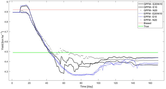
Figure 5.
Predicted yield of the proposed method (GPFM) for selected combinations in case study #1. The yield predictions for the true model (bold green line), biased model (solid red line), and EPFM (blue lines) are shown for comparison.
The water content predictions were barely improved by either method in all the tests (not shown), which can be explained by the fact that, as noted above, the two parameters related to root water extraction, SxBotQ and SxTopQ, were adjusted only marginally.
4.2. Case Study #2
Case study #1 was somewhat unrealistically simplistic in the sense that the soil was perfectly modeled. By comparison, in this second case study, the ‘true’ and ‘biased’ models differed in terms of six crop parameters and six soil parameters.
Compared to the ‘no-assimilation’ case, GPFM improved the estimation of canopy cover dramatically, as early as a few days after emergence, similarly to what was observed in Figure 2. Data assimilation also led to a much more accurate estimation of water content throughout the whole soil profile. This can be appreciated visually in Figure 6, which shows snapshots of the estimated water profile for three series of four consecutive days. Quantitative results are presented in Figure 7, which shows the sum of squared errors (SSE) between estimated and actual water content in each soil layer. The cyclic behavior observed for the biased model was due to the weekly irrigation events and is a clear indication of the inability of the model to correctly represent the system dynamics. By comparison, data assimilation reduced the modeling errors drastically in all three layers. Convergence toward the correct profile was notably faster in the bottom layer, which exhibited the slowest dynamics.

Figure 6.
True and estimated water content profiles with GPFM (blue dashed line) in an early period (days 10–13), intermediate period (days 30–33), and late period (days 50–53) in case study #2. The true profile (bold green line) and the profile estimated by the biased model (dashed red line) are shown for comparison.

Figure 7.
Sum of squared error (compared to the true model estimations) of the water content in each layer obtained with GPFM assimilation (solid line) and without assimilation (dashed line) in case study #2.
The convergence of the soil hydraulic parameters toward their true values can be appreciated in Figure 8. For the top and middle layers, data assimilation led to significant improvement in the estimations of and , and negligible improvement in the estimation of . For the bottom layer, significant improvement was achieved only for , while estimate worsened. These results can be explained by the fluctuations caused by irrigation in each layer (see also Figure 6)—in the top layer, the water content exhibited very large variations; in the middle layer, the water content fluctuated around field capacity; and in the bottom layer, the water content remained very close to field capacity. Overall, accurate estimation of appears to be much more challenging than that of the other parameters, which may be due to the influence of this parameter being low compared to other parameters, as observed in [37].

Figure 8.
Soil parameters of the true model (bold green line), biased model soil parameters (solid red line), and GPFM (ensemble average) (dashed black line) over time.
The time evolution of the estimation errors for the crop parameters is shown in Figure 9. Overall, the estimations of the crop parameters appeared to be more erratic than for the soil parameters (Figure 8). However, this was not entirely surprising, as not all the parameters chosen had a direct impact on the measured variables, and some of them were involved in the computations only during a certain period. On the other hand, the soil parameters influenced the water content along the whole simulation period. CCx and MaxRooting improved as they are influential parameters. CGC was not improved, despite its high influence on canopy cover. Both the large improvement of CCx and the low improvement of CGC agreed with the previous case studies where the parameter adjustments were small relative to state adjustment. Flowering, maturity, and HIstart have low influence of canopy cover, and hence poorer estimations were obtained for these parameters.

Figure 9.
Crop parameters of the true model (bold green line), biased model (solid red line), and GPFM (ensemble average) (dashed black line).
As in the previous case study, improved estimations of canopy cover and soil water content led to improved estimates of the final biomass and yield, as summarized in Table 7.
Table 7.
Yield and final biomass for the true model, the biased model without assimilation, and the biased model with data assimilation. (The number of parenthesis correspond to the relative error as a percentage.)
5. Conclusions
A framework integrating GA, PF, and MCMC for estimating parameters and state simultaneously was introduced. This framework, which was illustrated on two simulation examples with the crop model AquaCropOS, is generic and could be applied to any data assimilation application with any simulation model. The method was compared in two case studies with EPFM, in which the state and parameters were adjusted sequentially rather than simultaneously as in the present procedure. In the first case study, the proposed method led to more accurate estimations of the parameters and state, and improved the capability of the model to predict future crop development. Compared to EPFM, the superiority of the proposed method was more pronounced when used with large ensembles, as simultaneous estimation of the parameters and state enlarged the problem significantly. In the second case study, the method led to improved predictions of canopy cover, water content, final biomass, and yield. With respect to model parameters, whether or not a specific parameter was estimated accurately or not mostly depended on the influence that this parameter had on the measured variables. This indicates that rather than selecting parameters for adjustment “blindly”, as was done in this study (and in the literature), one should in fact select these parameters via sensitivity analysis.
Author Contributions
Conceptualization, A.J.; methodology, A.J. and R.L.; software, A.J.; validation, A.J.; formal analysis, A.J.; investigation, A.J.; resources, R.L.; writing—original draft preparation, A.J. and R.L.; writing—review and editing, R.L.; visualization, A.J.; supervision, R.L.; project administration, R.L.; funding acquisition, R.L. All authors have read and agreed to the published version of the manuscript.
Funding
The funding received from BARD, the United States-Israel Binational Agricultural Research and Development, to carry out this research work is sincerely acknowledged.
Acknowledgments
The authors wish to thank G. Sylaios for providing the data used in case study #1.
Conflicts of Interest
The authors declare no conflict of interest. The funders had no role in the design of the study; in the collection, analyses, or interpretation of data; in the writing of the manuscript; or in the decision to publish the results.
Symbols
| User-defined crossover parameter for state | |
| User-defined crossover parameter for parameters | |
| Above-ground biomass | |
| Canopy cover | |
| Initial canopy cover | |
| Maximum canopy cover | |
| Canopy decline coefficient | |
| Canopy growth coefficient | |
| Canopy size (adjusted for micro-advective effects) | |
| Average prediction error | |
| Error in parameter estimate (over an ensemble) averaged over time | |
| Reference evapotranspiration | |
| ( ) | Model |
| Water flowing into layer from the previous layer | |
| Water flowing from layer into the next layer and removed by the roots | |
| Measurements operator | |
| Harvest index | |
| Hydraulic conductivity at saturation | |
| Influence of temperature stress on biomass accumulation | |
| Crop-dependent coefficient used to express the impact of stress | |
| Number of the gene in the parameter vector within the particle | |
| Number of the gene in the state vector within the particle | |
| Likelihood | |
| True parameters | |
| Biased parameters | |
| Process noise covariance | |
| Measurements noise covariance | |
| SxBotQ | Maximum root water extraction at the bottom of the root zone |
| SxTopQ | Maximum root water extraction at top of the root zone |
| Length of the growing period | |
| Crop transpiration | |
| Forcing input | |
| True value of the state variable | |
| Water productivity | |
| State vector at time | |
| State obtained by crossover and mutation at time | |
| State of the parent particles with index | |
| The proposal state within particle at time | |
| Posterior state within particle at time | |
| Yield | |
| Vector of measurements | |
| Change in water amount in layer | |
| Gaussian noise for parameters mutation | |
| Gaussian noise for state mutation | |
| Vector of model parameters | |
| Water content at field capacity | |
| Water content at saturation | |
| Parameters within particle obtained by crossover and mutation at time | |
| Posterior parameter within particle at time | |
| Measurements noise | |
| Variance of parameters mutation noise | |
| Variance of state mutation noise | |
| Process noise | |
| Acronyms | |
| DSS | Decision support system |
| EKF | Extended Kalman filter |
| EPFM | Evolutionary particle filter combined with Monte Carlo Markov Chain |
| FAO | Food and Agriculture Organization |
| GA | Genetic algorithm |
| GPFM | Genetic-based particle filter combined with Monte Carlo Markov Chain |
| KF | Kalman filter |
| MA | Metaheuristic algorithm |
| MCMC | Monte Carlo Markov Chain |
| PF | Particle filter |
| UKF | Unscented Kalman filter |
References
- Raes, D.; Steduto, P.; Hsiao, T.C.; Fereres, E. AquaCrop—the FAO crop model to simulate yield response to water: II. Main algorithms and software description. Agron. J. 2009, 101, 438–447. [Google Scholar] [CrossRef]
- Steduto, P.; Hsiao, T.C.; Raes, D.; Fereres, E. AquaCrop—The FAO crop model to simulate yield response to water: I. Concepts and underlying principles. Agron. J. 2009, 101, 426–437. [Google Scholar] [CrossRef]
- Geerts, S.; Raes, D.; Garcia, M. Using AquaCrop to derive deficit irrigation schedules. Agric. Water Manag. 2010, 98, 213–216. [Google Scholar] [CrossRef]
- Linker, R.; Ioslovich, I.; Sylaios, G.; Plauborg, F.; Battilani, A. Optimal model-based deficit irrigation scheduling using AquaCrop: A simulation study with cotton, potato and tomato. Agric. Water Manag. 2016, 163, 236–243. [Google Scholar] [CrossRef]
- Li, F.; Yu, D.; Zhao, Y. Irrigation scheduling optimization for cotton based on the AquaCrop model. Agric. Water Manag. 2019, 33, 39–55. [Google Scholar] [CrossRef]
- Manivasagam, V.S.; Rozenstein, O. Practices for upscaling crop simulation models from field scale to large regions. Comput. Electron. Agric. 2020, 175, 105554. [Google Scholar] [CrossRef]
- Zhang, T.; Su, J.; Liu, C.; Chen, W.H. Bayesian calibration of AquaCrop model for winter wheat by assimilating UAV multi-spectral images. Comput. Electron. Agric. 2019, 167, 105052. [Google Scholar] [CrossRef]
- Evensen, G. Sequential data assimilation with a nonlinear quasi-geostrophic model using Monte Carlo methods to forecast error statistics. J. Geophys. Res. Oceans 1994, 99, 10143–10162. [Google Scholar] [CrossRef]
- Burgers, G.; van Leeuwen, P.J.; Evensen, G. Analysis scheme in the ensemble Kalman filter. Month Weather. Rev. 1998, 126, 1719–1724. [Google Scholar] [CrossRef]
- Kalman, R.E. A new approach to linear filtering and prediction problems. J. Basic Eng. 1960, 82, 35–45. [Google Scholar] [CrossRef]
- Jamal, A.; Linker, R. Inflation method based on confidence intervals for data assimilation in soil hydrology using ensemble Kalman filter. Vadose Zone J. 2019. [Google Scholar] [CrossRef]
- Wang, D.; Cai, X. Optimal estimation of irrigation schedule—An example of quantifying human interferences to hydrologic processes. Adv. Water Resour. 2007, 30, 1844–1857. [Google Scholar] [CrossRef]
- DeChant, C.M.; Moradkhani, H. Examining the effectiveness and robustness of sequential data assimilation methods for quantification of uncertainty in hydrologic forecasting. Water Resour. Res. 2012, 48. [Google Scholar] [CrossRef]
- Yan, H.; Moradkhani, H. Combined assimilation of streamflow and satellite soil moisture with the particle filter and geostatistical modeling. Adv. Water Res. 2016, 94, 364–378. [Google Scholar] [CrossRef]
- Evensen, G. Data Assimilation: The Ensemble Kalman Filter; Springer: Berlin/Heidelberg, Germany, 2009. [Google Scholar]
- Wang, D.; Chen, Y.; Cai, X. State and parameter estimation of hydrologic models using the constrained ensemble Kalman filter. Water Resour. Res. 2009, 45. [Google Scholar] [CrossRef]
- Yin, S.; Zhu, X. Intelligent particle filter and its application to fault detection of nonlinear system. IEEE Trans. Ind. Electron. 2015, 62, 3852–3861. [Google Scholar] [CrossRef]
- Abbaszadeh, P.; Moradkhani, H.; Yan, H. Enhancing hydrologic data assimilation by evolutionary particle filter and Markov chain Monte Carlo. Adv. Water Resour. 2018, 111, 192–204. [Google Scholar] [CrossRef]
- Berg, D.; Bauser, H.H.; Roth, K. Covariance resampling for particle filter–state and parameter estimation for soil hydrology. Hydrol. Earth Syst. Sci. 2019, 23, 1163–1178. [Google Scholar] [CrossRef]
- Chen, Y.; Cournède, P.H. Data assimilation to reduce uncertainty of crop model prediction with convolution particle filtering. Ecol. Model. 2014, 290, 165–177. [Google Scholar] [CrossRef]
- Moradkhani, H.; Hsu, K.L.; Gupta, H.; Sorooshian, S. Uncertainty assessment of hydrologic model states and parameters: Sequential data assimilation using the particle filter. Water Resour. Res. 2005, 41. [Google Scholar] [CrossRef]
- Qin, J.; Liang, S.; Yang, K.; Kaihotsu, I.; Liu, R.; Koike, T. Simultaneous estimation of both soil moisture and model parameters using particle filtering method through the assimilation of microwave signal. J. Geophys. Res. Atmos. 2009, 114. [Google Scholar] [CrossRef]
- Montzka, C.; Grant, J.P.; Moradkhani, H.; Franssen, H.J.H.; Weihermüller, L.; Drusch, M.; Vereecken, H. Estimation of radiative transfer parameters from L-band passive microwave brightness temperatures using advanced data assimilation. Vadose Zone J. 2013, 12, 1–17. [Google Scholar] [CrossRef]
- Andrieu, C.; Doucet, A.; Holenstein, R. Particle Markov chain Monte Carlo methods. J. R. Stat Soc. Ser. B 2010, 72, 269–342. [Google Scholar] [CrossRef]
- Moradkhani, H.; DeChant, C.M.; Sorooshian, S. Evolution of ensemble data assimilation for uncertainty quantification using the particle filter-Markov chain Monte Carlo method. Water Resour. Res. 2012, 48. [Google Scholar] [CrossRef]
- Kwok, N.M.; Fang, G.; Zhou, W. Evolutionary particle filter: Re-sampling from the genetic algorithm perspective. In Proceedings of the 2005 IEEE/RSJ International Conference on Intelligent Robots and Systems, Edmonton, AB, Canada, 2–6 August 2005; pp. 2935–2940. [Google Scholar]
- Valdes-Abellan, J.; Pachepsky, Y.; Martinez, G. MATLAB algorithm to implement soil water data assimilation with the Ensemble Kalman Filter using HYDRUS. MethodsX 2018, 5, 184–203. [Google Scholar] [CrossRef]
- Janikow, C.Z.; Michalewicz, Z. An experimental comparison of binary and floating point representations in genetic algorithms. In Proceedings of the 4th International Conference on Genetic Algorithms, San Diego, CA, USA, 13–16 July 1991; pp. 31–36. [Google Scholar]
- Magalhaes-Mendes, J. A comparative study of crossover operators for genetic algorithms to solve the job shop scheduling problem. WSEAS Trans. Comput. 2013, 12, 164–173. [Google Scholar]
- Park, S.; Hwang, J.P.; Kim, E.; Kang, H.-J. A New Evolutionary Particle Filter for the Prevention of Sample Impoverishment. IEEE Trans. Evol. Comput. 2009, 13, 801–809. [Google Scholar] [CrossRef]
- Price, J. Leaf area index estimation from visible and near-infrared reflectance data. Remote. Sens. Environ. 1995, 52, 55–65. [Google Scholar] [CrossRef]
- Soltani, A.; Galeshi, S. Importance of rapid canopy closure for wheat production in a temperate sub-humid environment: Experimentation and simulation. Field Crop. Res. 2002, 77, 17–30. [Google Scholar] [CrossRef]
- Pérez, G.; Coma, J.; Sol, S.; Cabeza, L. Green facade for energy savings in buildings: The influence of leaf area index and facade orientation on the shadow effect. Appl. Energy 2017, 187, 424–437. [Google Scholar] [CrossRef]
- Varella, H.; Guérif, M.; Buis, S.; Beaudoin, N. Soil properties estimation by inversion of a crop model and observations on crops improves the prediction of agro-environmental variables. Eur. J. Agron. 2010, 33, 139–147. [Google Scholar] [CrossRef]
- Varella, H.; Guérif, M.; Buis, S. Global sensitivity analysis measures the quality of parameter estimation: The case of soil parameters and a crop model. Environ. Model. Softw. 2010, 25, 310–319. [Google Scholar] [CrossRef]
- Nagarajan, K.; Judge, J.; Graham, W.; Monsivais-Huertero, A. Particle Filter-based assimilation algorithms for improved estimation of root-zone soil moisture under dynamic vegetation conditions. Adv. Water Resour. 2011, 34, 433–447. [Google Scholar] [CrossRef]
- Xu, X.; Sun, C.; Huang, G.; Mohanty, B.P. Global sensitivity analysis and calibration of parameters for a physically-based agro-hydrological model. Environ. Model. Softw. 2016, 83, 88–102. [Google Scholar] [CrossRef]
Publisher’s Note: MDPI stays neutral with regard to jurisdictional claims in published maps and institutional affiliations. |
© 2020 by the authors. Licensee MDPI, Basel, Switzerland. This article is an open access article distributed under the terms and conditions of the Creative Commons Attribution (CC BY) license (http://creativecommons.org/licenses/by/4.0/).