
Article

Individualized Prediction of Recurrence Following Uterine-Preserving Pelvic Organ Prolapse Repair Using Internally Validated Machine Learning Models

1
Department of Business Administration, Guilford Glazer Faculty of Business and Management, Ben-Gurion University of the Negev, Beer Sheba 8410501, Israel
2
Division of Urogynecology, Department of Obstetrics and Gynecology, Hadassah Medical Organization and Faculty of Medicine, Hebrew University of Jerusalem, Jerusalem 9112001, Israel
3
Faculty of Business Administration, Ono Academic College, Kiryat Ono 5545001, Israel
*
Author to whom correspondence should be addressed.
These authors contributed equally to this work.
J. Clin. Med. 2026, 15(16), 6366; https://doi.org/10.3390/jcm15166366
Submission received: 18 June 2026 / Revised: 25 July 2026 / Accepted: 4 August 2026 / Published: 18 August 2026
(This article belongs to the Special Issue Recent Clinical Advances in Pelvic Organ Prolapse)

Abstract

Background/Objectives: Approximately 11–20% of women affected by pelvic organ prolapse (POP) will undergo surgical intervention during their lifetime and nearly one-third of these women will require an additional procedure due to recurrence or failure of the initial repair. This study aimed to identify risk factors for failure and to develop models to predict subjective, anatomical, and composite failure after primary uterine-preserving POP surgery. Methods: We performed a retrospective cohort study of women undergoing primary uterine-preserving POP repair at a tertiary academic medical center between 2010 and 2024. Failure outcomes were defined as: subjective failure (patient-reported prolapse symptoms), anatomical failure (prolapse beyond the hymen during exam), and composite failure (subjective and/or anatomical failure and/or reoperation for prolapse). Risk factors were evaluated using univariable and multivariable logistic regression with odds ratios and 95% confidence intervals. Prediction models were trained in Python and internally validated using bootstrap optimism correction (500 resamples). Discrimination, overall accuracy, and calibration were evaluated. Results: Among 277 women, subjective failure occurred in 36 (13.0%), anatomical failure in 24 (8.7%), and composite failure in 46 (16.6%). In multivariable risk-factor models, larger genital hiatus was associated with higher odds of failure across endpoints and posterior compartment descent was independently associated with anatomical and composite failure. After bootstrap optimism correction, discrimination remained high for the best-performing models. Conclusions: In this single-center cohort, independent risk factors for failure after primary prolapse surgery were identified and prediction models showed strong internal discrimination. However, calibration limitations necessitate recalibration and external validation before clinical implementation.

1. Introduction

Pelvic floor dysfunction (PFD) encompasses a spectrum of debilitating conditions affecting women, including pelvic organ prolapse (POP), urinary incontinence, voiding dysfunction, and defecatory disorders [1]. These conditions impose a substantial burden on affected individuals and healthcare systems, with US prevalence estimates indicating that over one-third of parous women experience at least one PFD symptom by midlife [2].
Initial management emphasizes conservative approaches such as pelvic floor muscle training and pessary use; however, approximately 200,000 US women undergo POP surgery annually, with native-tissue repairs favored for their durability in select cases despite elevated recurrence risks [3].
Recurrence rates following primary surgery range from 13 to 30% at 1–2 years, varying by definition (subjective symptoms, anatomical stage ≥ 2, or reoperation) and are influenced by patient factors (age, parity, obesity), anatomical features (prolapse stage, levator integrity), and procedural elements (compartment addressed, concomitant repairs) [4,5]. Key risk factors include advanced preoperative prolapse, levator ani avulsion, enlarged genital hiatus, and posterior/apical defects, yet these predictors account for limited prognostic variance in isolation [6,7,8].
Despite recognition of these risks, validated tools for individualized recurrence prediction remain scarce, limiting preoperative counseling, surgical planning, and tailored surveillance [9]. Existing nomograms demonstrate moderate discrimination (c-statistic 0.70–0.85) but suffer from overfitting, poor calibration in external cohorts, and reliance on imaging or specialized metrics unavailable in routine practice [10,11]. Machine learning approaches, leveraging routinely collected POP-Q data, hold potential to enhance accuracy but require rigorous internal validation to mitigate optimism bias prior to clinical deployment [12].
Uterine-preserving procedures during POP repair are a viable surgical option promoted in recent years by both caregivers and patients. Advantages include shorter operative time, reduced intraoperative blood loss, and shorter hospital stay compared to apical prolapse repair involving hysterectomy [13,14]. However, data regarding risk factors for recurrence within this specific group is sparse.
The aim of the current study was to (1) delineate independent risk factors for subjective, anatomical, and composite POP recurrence following primary uterine-preserving apical prolapse repair and (2) derive a bootstrap-validated machine learning prediction model using preoperative/perioperative variables from a real-world cohort. These models aim to establish a foundation for individualized risk stratification; prospective external validation and recalibration are required before clinical deployment.

2. Materials and Methods

2.1. Study Design and Setting

We performed a retrospective cohort study at a tertiary university-affiliated teaching hospital. The study included women who underwent primary uterine-preserving apical prolapse repair between 2010 and 2024.

2.2. Participants

Eligible patients were women diagnosed with POP, including apical prolapse, who underwent primary uterine-preserving surgical repair. Patients with prior pelvic surgery for prolapse/incontinence were excluded. Procedures were performed as part of routine clinical care and included laparoscopic uterosacral ligament suspension, sacrospinous hysteropexy, vaginal colposuspension utilizing the Uphold Lite Mesh System (Boston Scientific, Springfield, MA, USA) and laparoscopic sacrohysteropexy. Concomitant procedures were performed as indicated and included anterior and posterior colporrhaphy, and mid-urethral sling procedures for stress incontinence.

2.3. Data Sources and Variables

Data were obtained from electronic medical records and operative reports. Preoperative variables included demographics, past medical, surgical and obstetric history (e.g., parity and delivery characteristics), lifestyle factors (smoking, sexual activity), menopausal status, and POP-Q measurements (Aa, Ba, Ap, Bp, C, D, genital hiatus [GH], perineal body [PB], and total vaginal length [TVL]) recorded using standardized POP-Q terminology. Operative variables included apical procedure type and the performance of concomitant procedures (e.g., anterior cystocele repair when applicable).

2.4. Outcomes

Three binary outcomes were defined: (1) Subjective failure: presence of patient-reported prolapse symptoms at follow-up. (2) Anatomical failure: evidence of prolapse beyond the hymen on physical examination. (3) Composite failure: subjective and/or anatomical failure and/or documented reoperation for prolapse. Follow-up routine care included visits at approximately 6 and 12 months postoperatively and annually thereafter when available. Given the variable follow-up duration across the 2010–2024 study period, recurrence was analyzed as a binary outcome rather than using time-to-event methods; this approach does not account for differences in observation time between patients and should be considered a limitation when interpreting absolute failure rates.

2.5. Statistical Analysis

Baseline characteristics were compared between outcome groups for each endpoint. Categorical variables were assessed using the chi-square test (or Fisher’s exact test when expected cell counts were small), and continuous variables were evaluated using the independent-samples t-test. Corresponding p-values are reported for descriptive comparisons.

2.6. Risk-Factor Models

Risk factors for each endpoint were evaluated using logistic regression. We estimated univariable models for each candidate predictor and a multivariable model incorporating the selected covariates. Effects are reported as odds ratios (ORs) with 95% confidence intervals (CIs).

2.7. Prediction Models

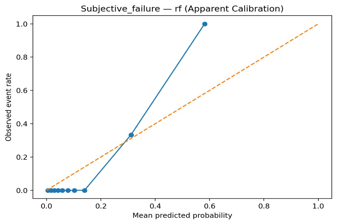
For each endpoint, prediction models were trained in Python 3.10 using penalized logistic regression, random forest, and gradient boosting (LightGBM). Internal validation was performed using bootstrap resampling (500 iterations with replacement) to estimate optimism-corrected performance. In each bootstrap sample, the full modeling pipeline—including feature preprocessing and, where applicable, hyperparameter selection—was refitted and evaluated both within the resampled dataset and in the original cohort to quantify overfitting. Missing covariate values were handled using median imputation for continuous variables and mode imputation for categorical variables; imputation parameters were estimated within each bootstrap resample to prevent information leakage. The optimism estimate, defined as the mean difference between bootstrap and original sample performance, was subtracted from the apparent performance to obtain corrected estimates. Model performance was summarized using AUC and PR-AUC for discrimination, Brier score for overall accuracy, and calibration intercept/slope and calibration curves. Calibration figures and model performance summaries generated in Python were incorporated into the manuscript from the prespecified project output directory (Figure A1 and Figure A2).

3. Results

Between 2010 and 2024, a total of 277 women met the inclusion criteria and underwent primary uterine-preserving POP repair. The mean age at surgery was 60.4 years (SD 10.0), and the mean BMI was 26.0 kg/m2 (SD 4.1). Surgical procedures comprised laparoscopic uterosacral ligament suspension (LUSLS), sacrohysteropexy, sacrospinous hysteropexy (SSL), and vaginal mesh repair using the Uphold system, with LUSLS representing the most common approach. Concomitant procedures were frequently performed, including anterior colporrhaphy, posterior repair, and mid-urethral sling placement. Postoperative follow-up was conducted at 6 and 12 months and annually thereafter as part of routine clinical care.
Subjective failure was assessed in 269 patients. As shown in Table 1, 36 patients (13.4%) experienced subjective failure, compared with 233 patients (86.6%) who did not. With respect to demographic characteristics, the mean BMI differed significantly between patients with and without subjective failure (p = 0.029). No medical comorbidities or prior delivery characteristics differed significantly between groups. For pelvic measurements, no preoperative or intraoperative attributes differed significantly between groups.
Anatomical failure was assessed in 268 patients. As shown in Table 2, 24 patients (9%) experienced anatomical failure, compared with 244 patients (91%) who did not. With respect to demographic characteristics, no attributes differed significantly between patients with and without anatomical failure. Regarding medical comorbidities, hyperthyroidism differed significantly by anatomical outcome (p = 0.012). For pelvic measurements, patients with anatomical failure had larger preoperative values for points C (p = 0.003), GH (p < 0.001), TVL (p < 0.001), Ap (p = 0.01), and Bp (p < 0.001) compared with patients without anatomical failure. No other attributes differed significantly between groups.
Composite failure was assessed in 270 patients. As shown in Table 3, 46 patients (17%) experienced composite failure, compared with 224 patients (83%) who did not. No demographic characteristics, medical comorbidities, or delivery characteristics differed significantly between groups. For pelvic measurements, patients with composite failure had larger preoperative values for points C (p = 0.05), GH (p = 0.005), TVL (p = 0.007), and Bp (p = 0.002) compared with patients without composite failure. No other attributes differed significantly between groups.

3.1. Risk Factors for Recurrence Following Primary Surgical Correction of Pelvic Organ Prolapse

We evaluated risk factors for distinct failure endpoints: subjective, anatomical, and composite, following primary POP surgery using logistic regression models and report effects as odds ratios (ORs). We estimated univariable models for each candidate predictor and a multivariable model incorporating the selected covariates. Candidate predictors were drawn from three prespecified domains: (1) demographic and anthropometric characteristics (e.g., age and BMI); (2) factors previously identified in the literature as significant predictors of failure after primary POP surgery; and (3) variables demonstrating statistically significant differences between patients who experience failure and those who do not. We acknowledge that the inclusion of criterion (3) introduces outcome-driven variable selection, which may constitute data leakage and inflate apparent model performance; this should be considered a limitation when interpreting results. Predictors with empty cells (zero observations in at least one outcome group) were excluded from regression analyses to ensure estimability and stable inference. Because no failures occurred among smokers, smoking was excluded due to complete separation (zero events), which precluded reliable model estimation.
Given the modest event counts (anatomical failure: 24 events; subjective failure: 36 events; composite failure: 46 events), the events-per-variable (EPV) ratio in the full multivariable models was limited, increasing the risk of overfitting and contributing to the wide confidence intervals observed for several coefficient estimates. We prioritized clinical plausibility and limited model complexity. As a sensitivity analysis, we fit a parsimonious adjusted model including age, BMI, procedure type, GH, and Bp, and compared estimates to the full model to assess robustness.

3.2. Risk Factors for Subjective Failure

The results of the multivariable logistic regression analysis for subjective failure are shown in Table 4. BMI and preoperative GH were independently associated with the outcome. After adjustment for age, procedure type, preoperative POP-Q measures (Aa, Ba, Ap, Bp, C, D, PB, TVL), and concomitant anterior (cystocele) repair, higher BMI was associated with lower odds of subjective failure (adjusted OR, 0.87 per 1 kg/m2 increase; 95 confidence interval, 0.77–0.98; p = 0.026), whereas larger GH was associated with higher odds of subjective failure (adjusted OR, 1.94 per 1 cm increase; 95 confidence interval, 1.02–3.66; p = 0.041). All preoperative POP-Q measures, including Ba, were entered into the multivariable model as part of the prespecified POP-Q adjustment set (domains 1 and 2); Ba was not selected based on its univariable significance. Although point Aa was associated with subjective failure in univariable analysis, it was not statistically significant after adjustment (adjusted OR, 0.67 per 1 cm increase; 95% confidence intervals, 0.42–1.05; p = 0.080). No other covariates were significantly associated with subjective failure in the adjusted model (all p > 0.05).

3.3. Risk Factors for Anatomical Failure

Multivariable logistic regression results for anatomical failure are presented in Table 5. Preoperative GH and Bp were independently associated with the outcome. After adjustment for age, BMI, comorbidities, procedure type, preoperative POP-Q measures, and concomitant anterior (cystocele) repair, larger GH was associated with higher odds of anatomical failure (adjusted OR, 3.55 per 1 cm increase; 95 confidence interval, 1.75–7.58; p = 0.001), and higher Bp was similarly associated with increased odds of anatomical failure (adjusted OR, 1.53 per 1 cm increase; 95 confidence interval, 1.14–2.12; p = 0.007). POP-Q point Ap and POP-Q point D were also statistically significant in the adjusted model (Ap: adjusted OR, 0.53 per 1 cm increase; 95 confidence intervals, 0.27–0.96; p = 0.047; D: adjusted OR, 0.58 per 1 cm increase; 95 confidence intervals, 0.35–0.95; p = 0.032).
Hyperthyroidism was associated with markedly higher odds of anatomical failure (adjusted OR, 23.24; 95 confidence intervals, 1.33–623.79; p = 0.027); however, given the small number of patients with hyperthyroidism, this estimate should be interpreted cautiously. No other covariates were significantly associated with anatomical failure after adjustment (all p > 0.05).

3.4. Risk Factors for Composite Failure

Multivariable logistic regression results for the composite outcome are presented in Table 6. Preoperative Bp and GH were independently associated with the outcome. After adjustment for age, BMI, procedure type, preoperative POP-Q measures, and concomitant anterior (cystocele) repair, higher Bp was associated with increased odds of the composite outcome (adjusted OR, 1.31 per 1 cm increase; 95 confidence interval, 1.03–1.70; p = 0.031), and larger GH was similarly associated with increased odds (adjusted OR, 1.79 per 1 cm increase; 95% confidence interval, 1.02–3.12; p = 0.040). POP-Q point Ap demonstrated a borderline association after adjustment (adjusted OR, 0.66 per 1 cm increase; 95% confidence intervals, 0.41–1.02; p = 0.074). No other covariates were significantly associated with the composite outcome in the adjusted model (all p > 0.05).

3.5. Predictive Models

Prediction models were developed to estimate the probability of subjective, anatomical, and composite failure after primary POP surgery. Candidate predictors reflected routinely collected clinical variables (demographic characteristics, surgical approach, and preoperative POP-Q measures) that are available for perioperative risk stratification. Models were trained in Python using penalized logistic regression, random forest, and gradient boosting (LightGBM) and internally validated using bootstrap optimism correction (500 resamples). Model performance was summarized using AUC and PR-AUC for discrimination, Brier score for overall accuracy, and calibration measures (intercept/slope and calibration plots). Given the modest event rates, PR-AUC was emphasized as a complementary measure to AUC.

3.6. Optimism-Corrected Prediction Performance

All performance estimates reflect bootstrap optimism correction as described in the Methods section and therefore represent internally validated performance rather than apparent (in-sample) estimates. Calibration-in-the-large (intercept), as shown in Table 7, reflects whether predictions are systematically too high or too low; values far from 0 indicate overall miscalibration. The calibration slope reflects whether predicted risks are too extreme (<1) or too moderate (>1). In this cohort, several models showed substantial intercept deviations, indicating that raw predicted probabilities would require recalibration before clinical use despite strong discrimination.

3.7. Model Explainability Using SHAP (Global Feature Attribution)

To improve the interpretability of the machine learning models, we summarized global feature contributions using Shapley additive explanations (SHAP). SHAP values quantify each predictor’s marginal contribution to the model output for each individual, allowing aggregation into global importance (mean absolute SHAP) and visualization of effect directionality (beeswarm plots). Because SHAPs are inherently model-specific and not causal, results are interpreted as patterns of model reliance rather than causal effects.

3.8. SHAP Values for Subjective, Anatomical and Composite Failure

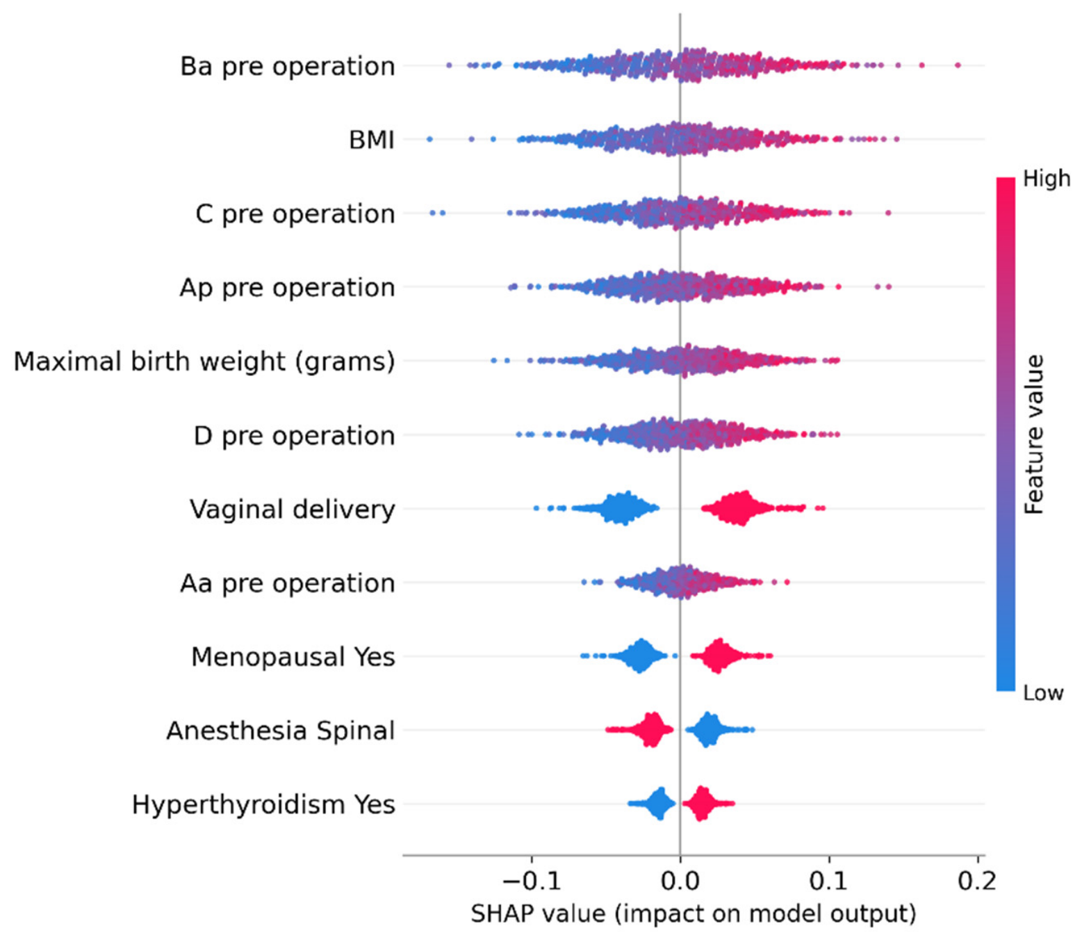
Table 8 summarizes the most influential predictors in the Subjective failure model, ranked by mean absolute SHAP value (mean(|SHAP|)). Mean(|SHAP|) reflects the average magnitude of each feature’s contribution to the model’s predictions across all patients, irrespective of direction (i.e., it indicates importance, not whether the feature increases or decreases risk). The leading predictors were preoperative prolapse measurements, particularly Ba (0.034) and C (0.029), together with BMI (0.031) and Ap (0.026). Maximal birth weight (0.024) and preoperative D (0.022) also contributed meaningfully, while vaginal delivery history showed a moderate contribution (0.016). Overall, the prominence of multiple preoperative POP-Q points (Ba, C, Ap, D, and Aa) indicates that baseline anatomic severity drives a substantial portion of the model’s predictive signal, with patient anthropometrics (BMI) and obstetric history (maximal birth weight, vaginal delivery) providing additional information. In contrast, Aa (0.009), menopausal status (0.008), and spinal anesthesia (0.002) had relatively small average impact on predictions, suggesting limited incremental value beyond the core anatomic and anthropometric predictors. Directionality and patient-specific effects should be interpreted using SHAP dependence plots or individual explanation plots rather than this global ranking alone (Figure 1 and Figure 2). Notably, genital hiatus (GH), which was the primary independent predictor in logistic regression analysis, does not appear among the top SHAP features in the machine learning model. This discrepancy reflects the distinct mechanisms by which these two approaches allocate predictive weight—logistic regression adjusts for collinear predictors sequentially, whereas machine learning models may distribute the predictive signal of correlated variables across multiple features. These rankings are therefore exploratory and should not be interpreted as definitive measures of clinical importance or as contradicting the logistic regression findings.
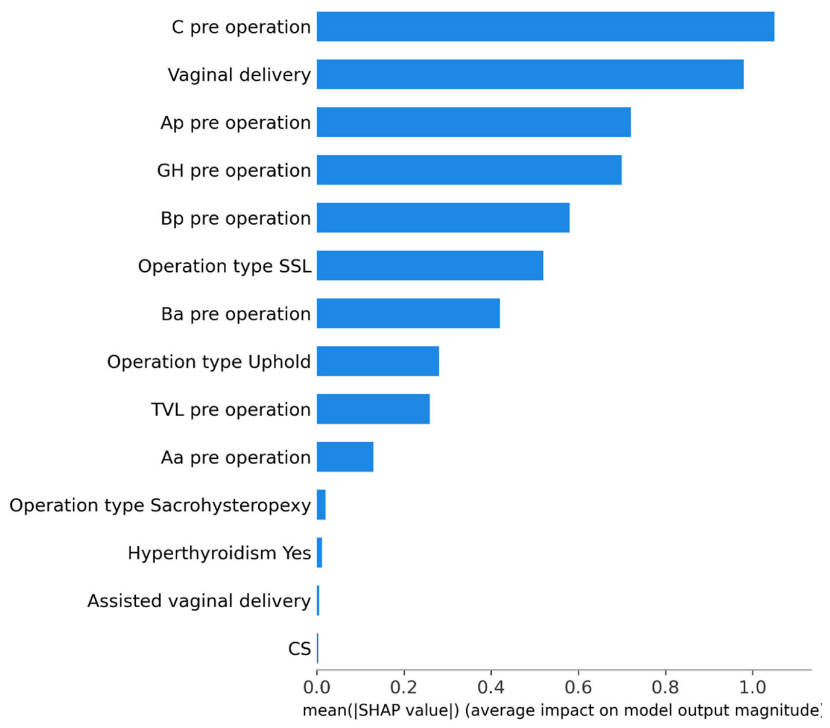
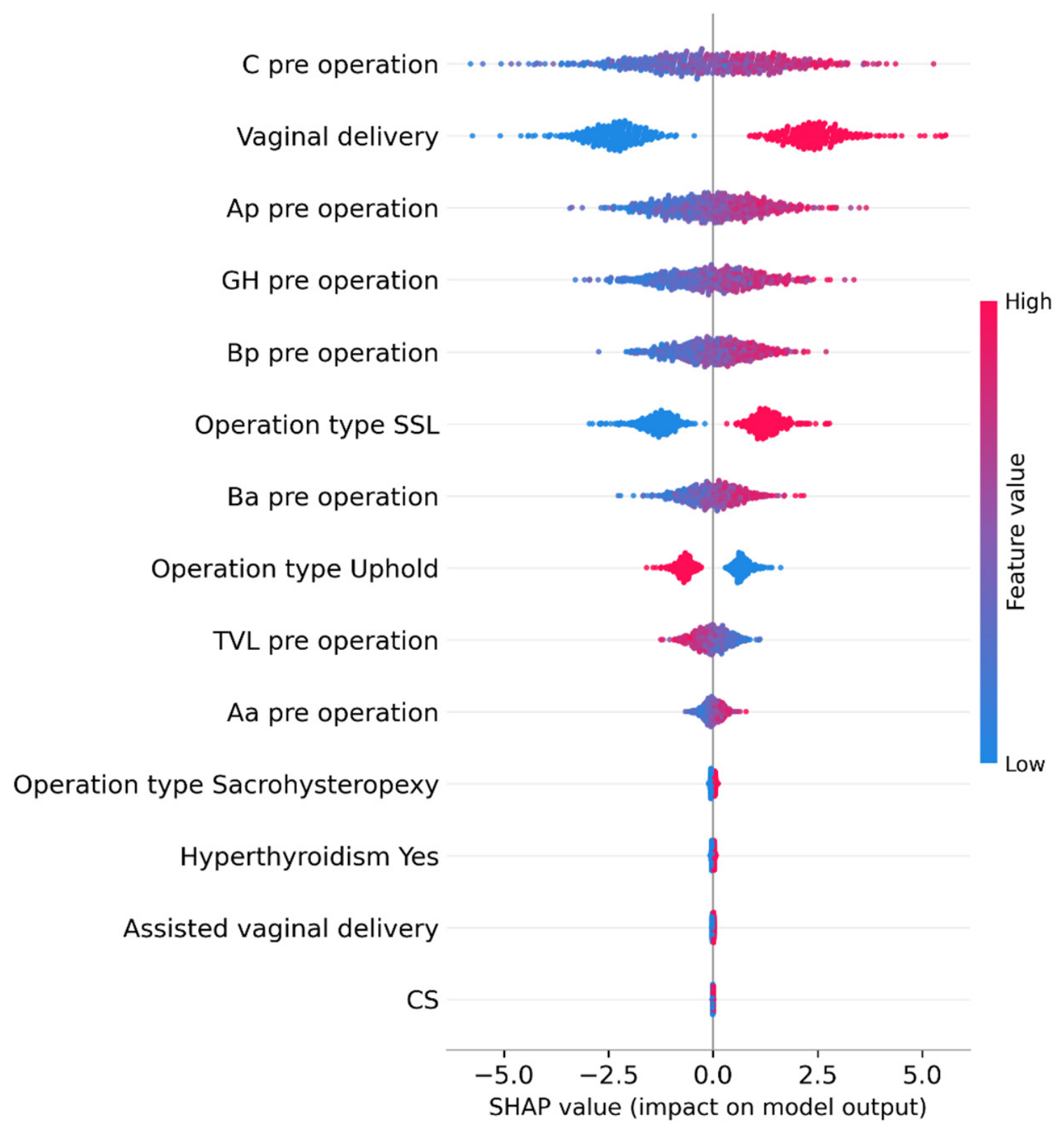
Table 9 summarizes the most influential predictors in the anatomical failure model, ranked by mean absolute SHAP value (mean(|SHAP|)). The dominant predictor was the preoperative C point (1.109), followed by vaginal delivery history (0.990). Additional high-impact anatomic measures included Ap (0.720), genital hiatus (GH; 0.711), perineal body (Bp; 0.572), Ba (0.447), total vaginal length (TVL; 0.282), and Aa (0.139), underscoring that baseline pelvic support and compartment-specific severity drive a substantial share of the model’s predictive signal. Notably, the surgical approach also contributed meaningfully: operation type SSL (0.561) and Uphold (0.292) ranked among the top predictors, suggesting that procedural selection provides incremental information beyond preoperative anatomy and obstetric history. Directionality and patient-specific effects should be interpreted using SHAP dependence plots or individual explanation plots rather than this global ranking alone (Figure 3 and Figure 4).
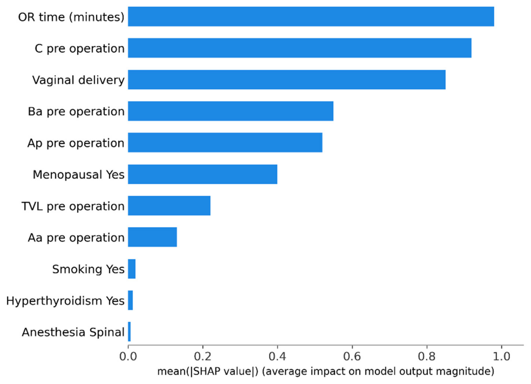
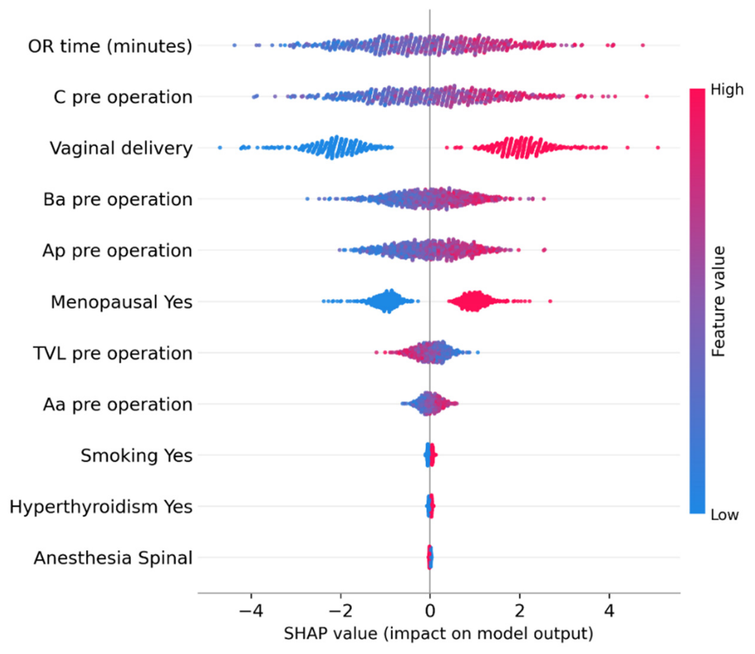
Table 10 summarizes the most influential predictors in the Composite outcome model, ranked by mean absolute SHAP value (mean(|SHAP|)). The most influential variable was operative time (OR time, minutes; 0.989), followed by the preoperative C point (0.951) and vaginal delivery history (0.843). Key anatomic measures, Ba (0.544), Ap (0.538), TVL (0.235), and Aa (0.135), also ranked among the top predictors, indicating that baseline pelvic support remains a major driver of the model’s predictive signal. Menopausal status contributed a moderate additional impact (0.404), suggesting incremental information beyond anatomy and operative factors. In contrast, smoking status and spinal anesthesia had mean(|SHAP|) values of 0.000, indicating a negligible contribution in this model and dataset. Directionality and patient-specific effects should be interpreted using SHAP dependence plots or individual explanation plots rather than this global ranking alone (Figure 5 and Figure 6).
Across endpoints, SHAPs indicated that model predictions were driven primarily by baseline pelvic support parameters (POP-Q) and select clinical/operative factors, consistent with the clinical premise that preoperative anatomy encodes substantial recurrence risk. Global importance rankings (mean absolute SHAP) were dominated by POP-Q landmarks reflecting apical support and vaginal caliber (e.g., C, GH/TVL when included), with additional contributions from compartment-specific descent measures and obstetric history variables. Importantly, SHAP patterns represent how the fitted model allocates predictive weight in this cohort and should not be interpreted as causal effects.
Across endpoints, global SHAP rankings indicated that baseline POP-Q parameters (apical position C, genital hiatus, and posterior compartment measures) dominated model predictions, suggesting that preoperative anatomic severity encodes substantial recurrence risk. Operative time emerged as an important feature for the composite model, which may function as a proxy for surgical complexity rather than a causal driver.

4. Discussion

In this retrospective cohort of women undergoing primary uterine-preserving POP surgery, we identified clinically interpretable risk factors for failure across subjective, anatomical, and composite endpoints and embedded internally validated prediction outputs generated in Python. Across endpoints, larger genital hiatus emerged as a consistent risk factor and posterior compartment descent was independently associated with anatomical and composite failure. These findings suggest that baseline pelvic floor metrics—particularly hiatal dimensions and posterior support—may be relevant for preoperative risk stratification; however, given the retrospective single-center design and modest event counts, these associations should be considered preliminary and require prospective external validation before informing routine counseling or surgical planning.
Large genital hiatus and posterior compartment defects may reflect significant obstetric trauma, potentially increasing the risk of subsequent POP. These findings may also indicate underlying connective tissue weakness, which could predispose affected women to higher rates of surgical failure.
Internally validated prediction models demonstrated strong optimism-corrected discrimination for all three endpoints. However, calibration performance was suboptimal across several models: calibration intercepts and slopes deviated notably from ideal values, indicating that predicted probabilities may systematically overestimate or underestimate true event risk. This miscalibration represents a critical limitation for clinical translation—a poorly calibrated model cannot reliably convey accurate absolute risk estimates to patients, limiting its utility for shared decision-making. Accordingly, statements regarding readiness for perioperative decision-support are premature, and the current findings should be interpreted as demonstrating preliminary predictive performance only. Future work must prioritize recalibration, external validation in independent cohorts, and evaluation of clinical utility through formal decision-curve analysis before these models are considered suitable for bedside implementation.
Strengths of this study include standardized POP-Q assessment, evaluation of multiple clinically relevant endpoints, and internal validation of prediction performance. Limitations include the single-center design, modest event counts (particularly for anatomical failure), and absence of external validation. The calibration performance of several models was suboptimal, and these models are not suitable for direct clinical use without recalibration. Outcomes were analyzed as binary variables without accounting for variable follow-up durations, which limits the interpretation of absolute failure rates and precludes time-to-event analysis. Additionally, the inclusion of statistically significant baseline comparisons as candidate predictors introduces a degree of outcome-driven variable selection that may inflate apparent model performance. Although the overall sample size was relatively small, the population was intentionally restricted to primary uterine-preserving procedures. This clinical design focused on a specific patient population and enabled more coherent estimation of recurrence risk within a defined surgical context. Importantly, the identified risk patterns were consistent with established biomechanical mechanisms and previously reported clinical associations, supporting the representativeness and face validity of the findings. The internally validated prediction performance further suggests that, despite modest event counts, the dataset was sufficient to develop stable and clinically meaningful prognostic models. Thus, rather than reflecting a limitation alone, the focused cohort facilitated a methodologically rigorous transition from traditional association testing to individualized risk prediction within a real-world surgical population.
In this cohort of women undergoing primary uterine-preserving POP repair, recurrence was evaluated across three clinically relevant endpoints: subjective, anatomical, and composite. These endpoints reflect related but not identical clinical outcomes. Enlarged genital hiatus and posterior compartment descent were consistent and clinically interpretable predictors across outcomes, whereas most demographic and obstetric factors showed limited predictive value. Compared with previous studies, the present findings emphasize the limited predictive contribution of commonly used clinical variables when considered in isolation, and the advantage of combining multiple parameters into a single prediction framework. These results support the feasibility of machine learning-based risk stratification in urogynecological care; however, the current findings represent preliminary, internally validated evidence only. Prospective external validation, recalibration, and formal assessment of clinical impact are required before these models can be recommended for routine clinical use.

Author Contributions

S.M.: Conceptualization, methodology, formal analysis and validation, manuscript writing and editing. H.H.C.: Conceptualization, methodology, data collection, manuscript writing and editing.; R.Y.: Conceptualization, methodology, manuscript editing. T.M.-S.: Conceptualization, project management, methodology. D.S.: Conceptualization, methodology, manuscript writing and editing. All authors have read and agreed to the published version of the manuscript.

Funding

This research received no external funding.

Institutional Review Board Statement

The study was conducted in accordance with the Declaration of Helsinki and approved by the Hadassah Medical Center Institutional Review Board (protocol code IRB No. 0687-22-HMO, first approved on 16 February 2023, receive extension on 21 December 2025).

Informed Consent Statement

Patient consent was waived due to retrospective cohort study.

Data Availability Statement

Data is available upon reasonable request from the corresponding author.

Conflicts of Interest

The authors declare no conflicts of interest.

Appendix A. Calibration Plots for Selected Models
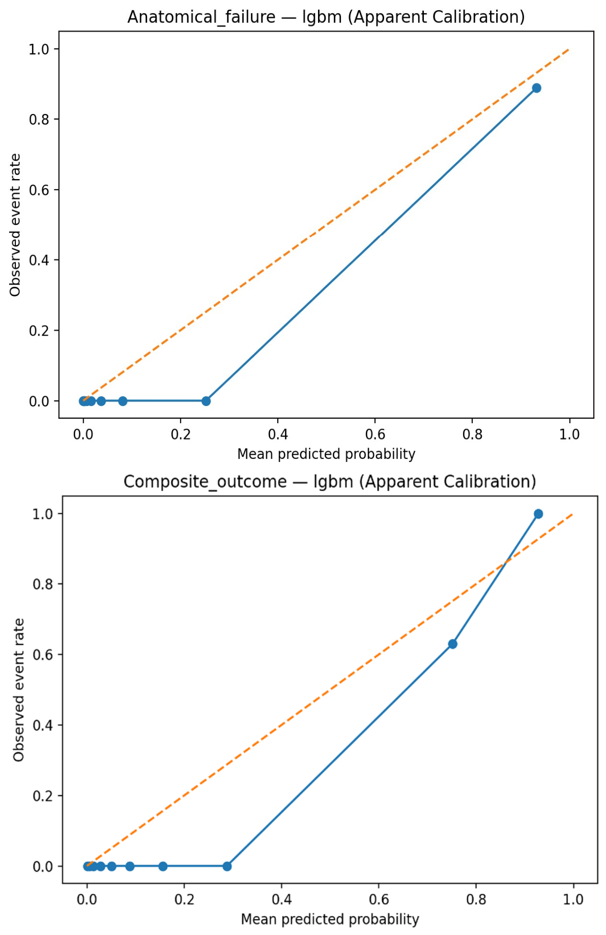
Figure A1. Apparent (in-sample) calibration plots for the three selected models: anatomical failure (LightGBM), composite outcome (LightGBM), and subjective failure (random forest). In each panel, the solid blue line with filled circles shows the observed event rate within bins of predicted risk plotted against the mean predicted probability of each bin, and the orange dashed diagonal line represents perfect calibration (predicted probability equal to observed event rate). Deviations of the blue curve from the diagonal indicate miscalibration: segments below the diagonal reflect overestimation of risk, whereas segments above it reflect underestimation.
Jcm 15 06366 g0a1aJcm 15 06366 g0a1b

Appendix B. Supplementary Discrimination Curves
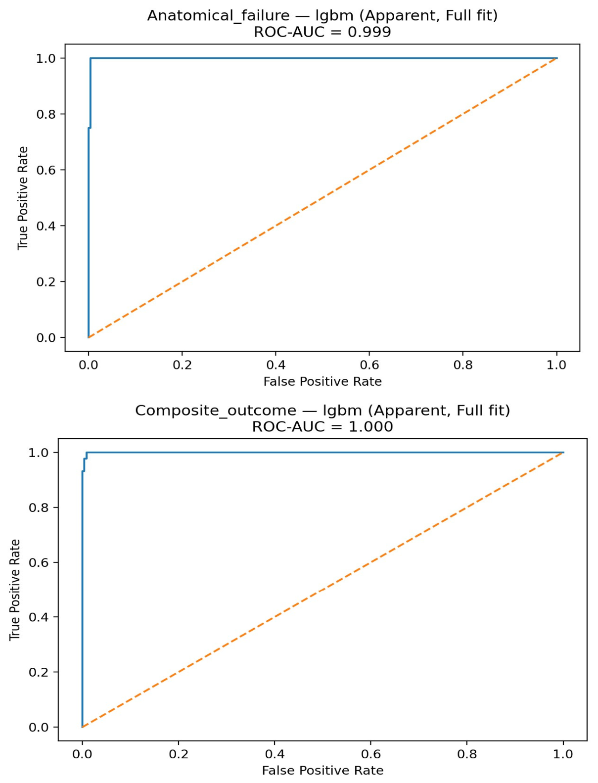
The following ROC curves are included to support the primary performance summary.
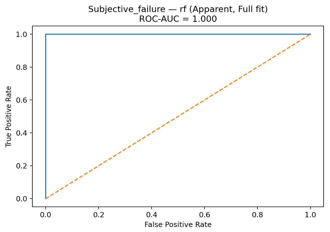
Figure A2. Apparent (full-fit) receiver operating characteristic (ROC) curves for the three selected models: anatomical failure (LightGBM; ROC-AUC = 0.999), composite outcome (LightGBM; ROC-AUC = 1.000), and subjective failure (random forest; ROC-AUC = 1.000). In each panel, the solid blue line is the ROC curve, plotting the true positive rate against the false positive rate across all classification thresholds, and the orange dashed diagonal line represents a random classifier with no discriminative ability (AUC = 0.5). Because these curves were derived from models fitted and evaluated on the full dataset without optimism correction, they overestimate discrimination relative to the internally validated performance reported in Table 7.
Jcm 15 06366 g0a2aJcm 15 06366 g0a2b

References

  1. Wu, J.M.; Hundley, A.F.; Fulton, R.G.; Myers, E.R. Forecasting the prevalence of pelvic floor disorders in U.S. women: 2010 to 2050. Obstet. Gynecol. 2009, 114, 1278–1283. [Google Scholar] [CrossRef] [Scilit] [PubMed]
  2. Nygaard, I.; Barber, M.D.; Burgio, K.L.; Kenton, K.; Ciucci, S.; Schaffer, J.; Spino, C.; Brody, D.J. Prevalence of symptomatic pelvic floor disorders in US women. JAMA 2008, 300, 1311–1316. [Google Scholar] [CrossRef] [Scilit] [PubMed]
  3. Maher, C.; Feiner, B.; Baessler, K.; Christmann-Schmid, C.; Haya, N.; Brown, J. Surgery for women with apical vaginal prolapse. Cochrane Database Syst. Rev. 2016, 10, CD012376. [Google Scholar] [CrossRef] [Scilit] [PubMed]
  4. Jeon, M.J.; Chung, S.M.; Jung, H.J.; Kim, S.K.; Bai, S.W. Risk Factors for the Recurrence of Pelvic Organ Prolapse. Gynecol. Obstet. Investig. 2008, 66, 268–273. [Google Scholar] [CrossRef] [Scilit] [PubMed]
  5. Shi, W.; Guo, L. Risk factors for the recurrence of pelvic organ prolapse: A meta-analysis. J. Obstet. Gynaecol. 2023, 43, 2160–2168. [Google Scholar] [CrossRef] [Scilit] [PubMed]
  6. Dietz, H.P.; Simpson, J.M. Levator trauma is associated with pelvic organ prolapse. BJOG Int. J. Obstet. Gynaecol. 2008, 115, 979–984. [Google Scholar] [CrossRef] [Scilit] [PubMed]
  7. Friedman, T.; Eslick, G.D.; Dietz, H.P. Risk factors for prolapse recurrence: Systematic review and meta-analysis. Ultrasound Obstet. Gynecol. 2018, 29, 13–21. [Google Scholar] [CrossRef] [Scilit] [PubMed]
  8. Bodner-Adler, B.; Bodner, K.; Carlin, G.; Kimberger, O.; Marschalek, J.; Koelbl, H.; Umek, W. Clinical risk factors for recurrence of pelvic organ prolapse after primary native tissue prolapse repair. Wien. Klin. Wochenschr. 2022, 134, 73–75. [Google Scholar] [CrossRef] [Scilit] [PubMed]
  9. Steyerberg, E.W.; Moons, K.G.M.; van der Windt, D.A.; Hayden, J.A.; Perel, P.; Schroter, S.; Riley, R.D.; Hemingway, H.; Altman, D.G. Prognosis research strategy (PROGRESS) 3: Prognostic model research. PLoS Med. 2013, 10, e1001381. [Google Scholar] [CrossRef] [Scilit] [PubMed]
  10. Zhang, P.; Du, W.; Guo, G.; Yuan, M.; Wei, J. Influencing factors of recurrence after pelvic organ prolapse surgery and construction of a nomogram risk prediction model. Rev. Assoc. Med. Bras. 2024, 70, e20240849. [Google Scholar] [CrossRef] [Scilit] [PubMed]
  11. Collins, G.S.; Reitsma, J.B.; Altman, D.G.; Moons, K.G.M. Transparent reporting of a multivariable prediction model for individual prognosis or diagnosis (TRIPOD): The TRIPOD statement. Ann. Intern. Med. 2015, 162, 55–63. [Google Scholar] [CrossRef] [Scilit] [PubMed]
  12. Payebto Zoua, E.; Boulvain, M.; Dällenbach, P. The distribution of pelvic organ support defects in women undergoing pelvic organ prolapse surgery and compartment specific risk factors. Int. Urogynecol. J. 2022, 33, 405–409. [Google Scholar] [CrossRef] [Scilit] [PubMed]
  13. Meriwether, K.V.; Antosh, D.D.; Olivera, C.K.; Kim-Fine, S.; Balk, E.M.; Murphy, M.; Grimes, C.L.; Sleemi, A.; Singh, R.; Dieter, A.A.; et al. Uterine preservation vs hysterectomy in pelvic organ prolapse surgery: A systematic review with meta-analysis and clinical practice guidelines. Am. J. Obstet. Gynecol. 2018, 219, 129–146.e2. [Google Scholar] [CrossRef] [Scilit] [PubMed]
  14. Chang, O.H.; Carter Ramirez, A.; Edwards, A.; Chill, H.H.; Letko, J.; Woodburn, K.L.; Cundiff, G.W. The Role of Uterine Preservation at the Time of Pelvic Organ Prolapse Surgery. Urogynecology 2025, 31, 482–495. [Google Scholar] [CrossRef] [Scilit] [PubMed]
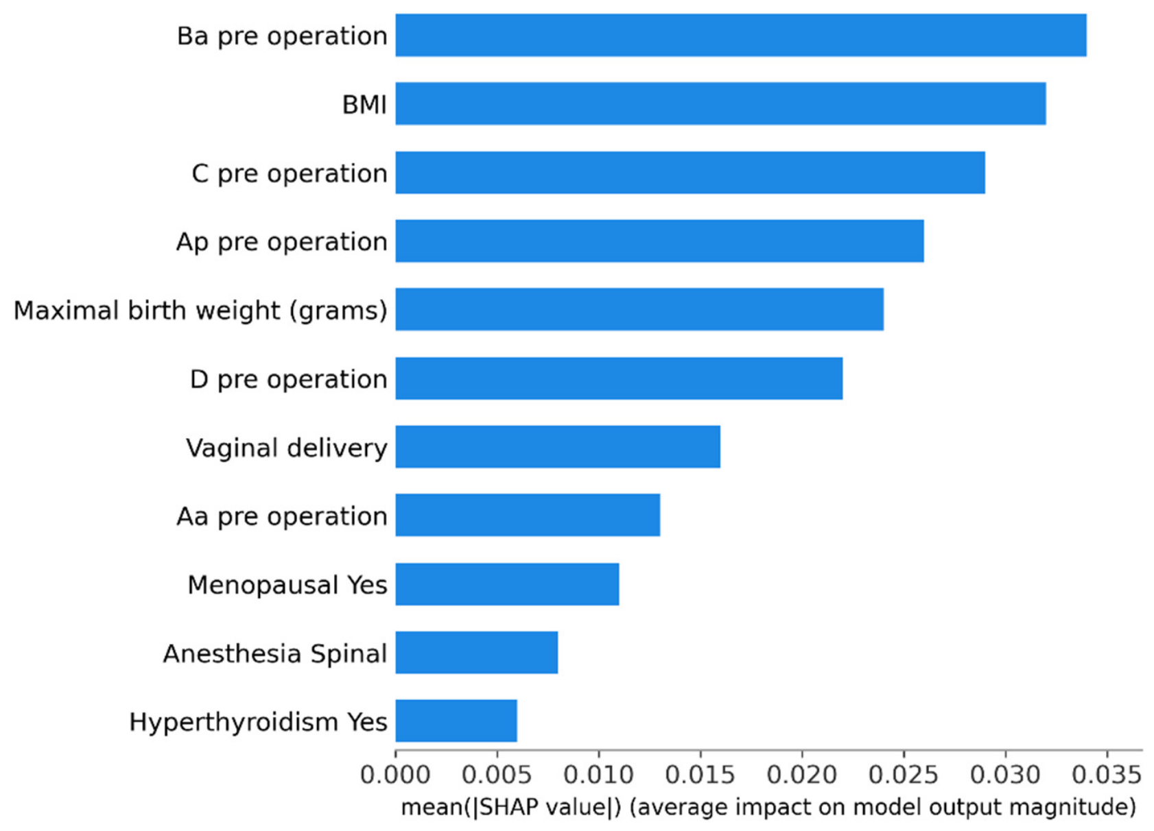
Figure 1. Global SHAP feature importance for subjective failure (random forest). Bar plot shows mean absolute SHAP values across all observations; larger values indicate greater overall contribution to the model prediction.
Jcm 15 06366 g001
Figure 2. SHAP beeswarm for subjective failure (random forest). Each point represents a patient; x-axis is the SHAP value (impact on predicted probability of failure), and color encodes the feature value (high vs. low).
Jcm 15 06366 g002
Figure 3. Global SHAP feature importance for anatomical failure (LightGBM). Bar plot shows mean absolute SHAP values across all observations; larger values indicate greater overall contribution to the model prediction.
Jcm 15 06366 g003
Figure 4. SHAP beeswarm for anatomical failure (LightGBM). Each point represents a patient; x-axis is the SHAP value (impact on predicted probability of failure), and color encodes the feature value (high vs. low).
Jcm 15 06366 g004
Figure 5. Global SHAP feature importance for composite outcome failure (LightGBM). Bar plot shows mean absolute SHAP values across all observations; larger values indicate greater overall contribution to the model prediction.
Jcm 15 06366 g005
Figure 6. SHAP beeswarm for composite outcome failure (LightGBM). Each point represents a patient; x-axis is the SHAP value (impact on predicted probability of failure), and color encodes the feature value (high vs. low).
Jcm 15 06366 g006
Table 1. Baseline characteristics by subjective failure.
Dependent: Subjective FailureNo
(n = 233)
Yes
(n = 36)
p
Age at operation60.4 (9.6)60.4 (13.1)0.979
BMI 26.1 (4.1)24.5 (3.1)0.029
Parity5.2 (3.0)4.5 (2.7)0.173
Vaginal delivery5.0 (3.0)4.4 (2.7)0.270
Cesarean delivery0.2 (0.5)0.1 (0.3)0.285
Assisted vaginal delivery19 (8.3)4 (11.1)0.805
Maximal birth weight (grams)3674.9 (517.5)3657.6 (867.9)0.871
Smoking11 (4.8)0 (0.0)0.375
Menopausal52 (22.7)13 (36.1)0.126
Sexually active145 (88.4)24 (92.3)0.801
Comorbidities
CHF1 (0.4)1 (2.8)0.628
Hyperthyroidism1 (0.4)2 (5.6)0.061
Arrythmia3 (1.3)1 (2.8)1.000
Atrial fibrillation3 (1.3)1 (2.8)1.000
Hypothyroidism26 (11.2)5 (13.9)0.844
Hypertension34 (14.6)7 (19.4)0.614
DM24 (10.3)1 (2.8)0.255
Prior pelvic surgery20 (8.6)2 (5.6)0.766
Previous incontinence surgery1 (0.4)0 (0.0)1.000
POP-Q
Aa pre-op2.4 (1.3)1.9 (1.7)0.036
Ba pre-op3.7 (2.0)3.8 (3.2)0.628
C pre-op0.1 (3.5)0.3 (4.9)0.689
GH pre-op4.9 (0.7)5.2 (1.2)0.051
PB pre-op3.0 (0.3)3.1 (0.2)0.359
TVL pre-op9.3 (0.6)9.5 (0.8)0.156
Ap pre-op−0.7 (1.3)−0.5 (1.9)0.323
Bp pre-op−0.4 (2.2)0.2 (3.5)0.172
D pre-op−4.6 (1.6)−4.9 (1.8)0.366
Pre-op hemoglobin13.2 (1.1)13.3 (1.3)0.623
Operation type 0.695
LUSLS119 (51.1)18 (50.0)
Sacrohysteropexy24 (10.3)4 (11.1)
SSLF56 (24.0)11 (30.6)
Uphold34 (14.6)3 (8.3)
Concomitant procedures
Mid-urethral sling120 (51.5)19 (52.8)1.000
Anterior repair 188 (80.7)29 (80.6)1.000
Posterior repair 178 (76.4)29 (80.6)0.735
Cervical amputation 24 (10.4)2 (5.6)0.539
Anesthesia 0.221
General217 (97.3)33 (91.7)
Spinal6 (2.7)3 (8.3)
OR time (minutes)122.3 (60.6)117.7 (81.4)0.716
Note: BMI, body mass index; CHF, chronic heart failure; DM, diabetes melitus; POP-Q, pelvic organ prolapse quantification system; LUSLS, laparoscopic uterosacral ligament suspension; SSLF, sacrospinous ligament fixation; OR, operating room.
Table 2. Baseline characteristics by anatomical failure.
Dependent: Anatomical FailureNo
(n = 244)
Yes
(n = 24)
p
Age at operation60.4 (10.0)60.6 (11.6)0.935
BMI25.8 (4.1)26.3 (4.1)0.557
Parity5.0 (2.9)5.8 (3.7)0.229
Vaginal delivery4.8 (2.9)5.6 (3.7)0.202
Cesarean delivery0.2 (0.5)0.2 (0.4)0.963
Assisted vaginal delivery22 (9.1)1 (4.2)0.658
Maximal birth weight (grams)3672.5 (564.9)3697.1 (680.0)0.843
Smoking11 (4.5)0 (0.0)0.597
Menopausal57 (23.8)8 (33.3)0.429
Sexually active155 (89.6)13 (81.2)0.548
Comorbidities
CHF1 (0.4)1 (4.2)0.425
Hyperthyroidism1 (0.4)2 (8.3)0.012
Arrythmia4 (1.6)0 (0.0)1.000
Atrial fibrillation3 (1.2)1 (4.2)0.802
Hypothyroidism29 (11.9)2 (8.3)0.853
Hypertension35 (14.3)6 (25.0)0.277
DM23 (9.4)2 (8.3)1.000
Prior pelvic surgery20 (8.2)2 (8.3)1.000
Previous incontinence surgery1 (0.4)0 (0.0)1.000
POP-Q
Aa pre-op2.3 (1.3)1.9 (1.8)0.173
Ba pre-op3.6 (1.9)4.7 (4.0)0.015
C pre-op−0.1 (3.3)2.1 (5.8)0.003
GH pre-op4.9 (0.7)5.7 (1.2)<0.001
PB pre-op3.0 (0.3)3.0 (0.3)0.817
TVL pre-op9.3 (0.6)9.8 (1.2)<0.001
Ap pre-op−0.7 (1.3)0.0 (2.1)0.010
Bp pre-op−0.6 (1.8)2.1 (4.9)<0.001
D pre-op−4.7 (1.6)−4.3 (2.3)0.320
Pre-op hemoglobin13.2 (1.1)13.2 (1.6)0.931
Operation type 0.054
LUSLS131 (53.7)6 (25.0)
Sacrohysteropexy25 (10.2)3 (12.5)
SSL57 (23.4)10 (41.7)
Uphold31 (12.7)5 (20.8)
Concomitant procedures
Mid-urethral sling127 (52.0)11 (45.8)0.713
Anterior repair 201 (82.4)16 (66.7)0.110
Posterior repair190 (77.9)17 (70.8)0.597
Cervical amputation24 (10.0)2 (8.3)1.000
Anesthesia 0.436
General228 (97.0)22 (91.7)
Spinal7 (3.0)2 (8.3)
OR time (minutes)121.0 (62.9)130.2 (71.7)0.557
Data presented as [mean ± SD] or [n (%)]. Note: BMI, body mass index; CHF, chronic heart failure; DM, diabetes melitus; POP-Q, pelvic organ prolapse quantification system; LUSLS, laparoscopic uterosacral ligament suspension; SSL, sacrospinous ligament fixation; OR, operating room.
Table 3. Baseline characteristics by composite outcome.
Dependent: Composite OutcomeNo
(n = 224)
Yes
(n = 46)
p
Age at operation60.5 (9.7)59.7 (11.9)0.622
BMI26.0 (4.1)25.1 (3.6)0.202
Parity5.1 (2.9)4.9 (3.1)0.665
Vaginal delivery4.9 (2.9)4.8 (3.1)0.840
Cesarean delivery0.2 (0.5)0.1 (0.3)0.428
Assisted vaginal delivery19 (8.6)4 (8.7)1.000
Maximal birth weight (grams)3687.9 (512.3)3614.9 (814.5)0.449
Smoking11 (5.0)0 (0.0)0.257
Menopausal49 (22.3)16 (34.8)0.108
Sexually active138 (88.5)32 (91.4)0.835
Comorbidities
CHF1 (0.4)1 (2.2)0.764
Hyperthyroidism1 (0.4)2 (4.3)0.127
Arrythmia3 (1.3)1 (2.2)1.000
Atrial fibrillation3 (1.3)1 (2.2)1.000
Hypothyroidism26 (11.6)5 (10.9)1.000
Hypertension32 (14.3)9 (19.6)0.494
DM23 (10.3)2 (4.3)0.326
Prior pelvic surgery20 (9.0)2 (4.3)0.456
Previous incontinence surgery1 (0.4)0 (0.0)1.000
POPQ
Aa pre-op2.3 (1.3)2.1 (1.6)0.256
Ba pre-op3.5 (1.9)4.3 (3.2)0.046
C pre-op−0.1 (3.3)0.9 (5.1)0.080
GH pre-op4.9 (0.7)5.2 (1.1)0.005
PB pre-op3.0 (0.3)3.1 (0.3)0.487
TVL pre-op9.3 (0.6)9.6 (0.9)0.007
Ap pre-op−0.7 (1.3)−0.5 (1.8)0.393
Bp pre-op−0.6 (1.9)0.6 (4.0)0.002
D pre-op−4.6 (1.6)−4.7 (1.8)0.931
Pre-op hemoglobin13.2 (1.1)13.3 (1.2)0.732
Operation type 0.601
LUSLS117 (52.2)20 (43.5)
Sacrohysteropexy24 (10.7)4 (8.7)
SSLF53 (23.7)14 (30.4)
Uphold30 (13.4)8 (17.4)
Concomitant procedures
Mid-urethral sling114 (50.9)25 (54.3)0.791
Anterior repair 183 (81.7)34 (73.9)0.314
Posterior repair174 (77.7)33 (71.7)0.499
Cervical amputation 23 (10.4)3 (6.5)0.592
Anesthesia 0.416
General209 (97.2)43 (93.5)
Spinal6 (2.8)3 (6.5)
OR time (minutes)123.1 (61.1)110.3 (75.6)0.270
Data presented as [mean ± SD] or [n (%)]. Note: BMI, body mass index, CHF, chronic heart failure, DM, diabetes melitus, POPQ, pelvic organ prolapse quantification system, LUSLS, laparoscopic uterosacral ligament suspension, SSLF, sacrospinous ligament fixation, OR, operating room.
Table 4. Logistic regression results for subjective failure (univariable and multivariable).
Dependent: Subjective FailureNo
(n = 233)
Yes
(n = 33)
OR (Univariable)OR (Multivariable)
Age at operation60.4 (9.6)60.4 (13.1)1.00 (0.97–1.04, p = 0.979)1.01 (0.96–1.06, p = 0.735)
BMI26.1 (4.1)24.5 (3.1)0.89 (0.80–0.98, p = 0.030)0.87 (0.77–0.98, p = 0.026)
Operation type
LUSLS119 (86.9)18 (13.1)--
Sacrohysteropexy24 (85.7)4 (14.3)1.10 (0.30–3.28, p = 0.871)1.34 (0.25–5.90, p = 0.715)
SSLF56 (83.6)11 (16.4)1.30 (0.56–2.90, p = 0.530)1.33 (0.45–3.77, p = 0.600)
Uphold34 (91.9)3 (8.1)0.58 (0.13–1.85, p = 0.409)0.54 (0.06–4.53, p = 0.567)
POPQ
Aa pre op2.4 (1.3)1.9 (1.7)0.79 (0.63–1.00, p = 0.040)0.67 (0.42–1.05, p = 0.080)
Ba pre-op3.7 (2.0)3.8 (3.2)1.04 (0.88–1.21, p = 0.626)1.32 (0.87–2.03, p = 0.196)
C pre-op0.1 (3.5)0.3 (4.9)1.02 (0.92–1.12, p = 0.688)0.87 (0.69–1.09, p = 0.249)
GH pre-op4.9 (0.7)5.2 (1.2)1.45 (0.98–2.11, p = 0.057)1.94 (1.02–3.66, p = 0.041)
PB pre-op3.0 (0.3)3.1 (0.2)1.81 (0.54–6.58, p = 0.357)1.84 (0.47–7.96, p = 0.400)
TVL pre-op9.3 (0.6)9.5 (0.8)1.39 (0.84–2.21, p = 0.946)1.03 (0.45–2.19, p = 0.166)
Ap pre-op−0.7 (1.3)−0.5 (1.9)1.13 (0.88–1.43, p = 0.323)0.95 (0.57–1.61, p = 0.860)
Bp pre-op−0.4 (2.2)0.2 (3.5)1.09 (0.95–1.22, p = 0.180)1.04 (0.76–1.37, p = 0.816)
D pre-op−4.6 (1.6)−4.9 (1.8)0.89 (0.68–1.12, p = 0.357)0.81 (0.55–1.15, p = 0.265)
Anterior repair188 (86.6)29 (13.4)0.99 (0.43–2.59, p = 0.985)0.68 (0.15–3.51, p = 0.628)
Data presented as [mean ± SD] or [n (%)]. Note: BMI, body mass index; POPQ, pelvic organ prolapse quantification system; LUSLS, laparoscopic uterosacral ligament suspension; SSLF, sacrospinous ligament fixation.
Table 5. Logistic regression results for anatomical failure (univariable and multivariable).
Dependent: Anatomical FailureNoYesOR (Univariable)OR (Multivariable)
Age at operation60.4 (10.0)60.6 (11.6)1.00 (0.96–1.05, p = 0.935)1.00 (0.94–1.06, p = 0.915)
BMI25.8 (4.1)26.3 (4.1)1.03 (0.93–1.13, p = 0.556)0.98 (0.84–1.12, p = 0.787)
Hyperthyroidism (Yes)1 (33.3)2 (66.7)22.09 (2.04–486.24, p = 0.013)23.24 (1.33–623.79, p = 0.027)
POPQ
Aa pre-op2.3 (1.3)1.9 (1.8)0.83 (0.64–1.11, p = 0.177)1.36 (0.73–2.79, p = 0.359)
Ba pre-op3.6 (1.9)4.7 (4.0)1.22 (1.03–1.45, p = 0.018)0.62 (0.34–1.08, p = 0.102)
C pre-op−0.1 (3.3)2.1 (5.8)1.15 (1.04–1.28, p = 0.005)1.17 (0.88–1.56, p = 0.287)
GH pre-op4.9 (0.7)5.7 (1.2)2.45 (1.61–3.91, p < 0.001)3.55 (1.75–7.58, p = 0.001)
PB pre-op3.0 (0.3)3.0 (0.3)1.18 (0.31–5.21, p = 0.816)0.84 (0.16–5.14, p = 0.840)
TVL pre-op9.3 (0.6)9.8 (1.2)2.16 (1.31–3.76, p = 0.003)1.89 (0.76–4.79, p = 0.163)
Ap pre-op−0.7 (1.3)0.0 (2.1)1.41 (1.07–1.83, p = 0.012)0.53 (0.27–0.96, p = 0.047)
Bp pre-op−0.6 (1.8)2.1 (4.9)1.31 (1.16–1.50, p < 0.001)1.53 (1.14–2.12, p = 0.007)
D pre-op−4.7 (1.6)−4.3 (2.3)1.11 (0.87–1.36, p = 0.323)0.58 (0.35–0.95, p = 0.032)
Operation type
LUSLS131 (95.6)6 (4.4)--
Sacrohysteropexy25 (89.3)3 (10.7)2.62 (0.53–10.64, p = 0.193)1.34 (0.12–10.66, p = 0.796)
SSLF57 (85.1)10 (14.9)3.83 (1.36–11.73, p = 0.013)3.35 (0.74–15.86, p = 0.117)
Uphold31 (86.1)5 (13.9)3.52 (0.96–12.44, p = 0.048)1.14 (0.08–22.37, p = 0.927)
Anterior repair201 (92.6)16 (7.4)0.43 (0.18–1.11, p = 0.068)0.38 (0.05–4.46, p = 0.382)
Data presented as [mean ± SD] or [n (%)]. Note: BMI, body mass index; POPQ, pelvic organ prolapse quantification system; LUSLS, laparoscopic uterosacral ligament suspension; SSLF, sacrospinous ligament fixation.
Table 6. Logistic regression results for composite outcome failure (univariable and multivariable).
Dependent: Composite OutcomeNoYesOR (Univariable)OR (Multivariable)
Age at operation60.5 (9.7)59.7 (11.9)0.99 (0.96–1.02, p = 0.620)0.99 (0.95–1.03, p = 0.543)
BMI26.0 (4.1)25.1 (3.6)0.95 (0.86–1.03, p = 0.202)0.92 (0.83–1.02, p = 0.120)
POPQ
C pre-op−0.1 (3.3)0.9 (5.1)1.08 (0.99–1.17, p = 0.082)0.95 (0.78–1.16, p = 0.617)
GH pre-op4.9 (0.7)5.2 (1.1)1.63 (1.14–2.35, p = 0.007)1.79 (1.02–3.12, p = 0.040)
PB pre-op3.0 (0.3)3.1 (0.3)1.49 (0.50–4.75, p = 0.485)1.27 (0.38–4.60, p = 0.705)
TVL pre-op9.3 (0.6)9.6 (0.9)1.75 (1.12–2.82, p = 0.014)1.20 (0.60–2.37, p = 0.598)
Aa pre-op2.3 (1.3)2.1 (1.6)0.88 (0.71–1.11, p = 0.257)0.88 (0.59–1.35, p = 0.560)
Ba pre-op3.5 (1.9)4.3 (3.2)1.15 (1.00–1.32, p = 0.049)1.08 (0.74–1.60, p = 0.680)
Ap pre-op−0.7 (1.3)−0.5 (1.8)1.10 (0.87–1.37, p = 0.393)0.66 (0.41–1.02, p = 0.074)
Bp pre-op−0.6 (1.9)0.6 (4.0)1.17 (1.05–1.31, p = 0.006)1.31 (1.03–1.70, p = 0.031)
D pre-op−4.6 (1.6)−4.7 (1.8)0.99 (0.80–1.19, p = 0.931)0.79 (0.56–1.09, p = 0.184)
Operation type
LUSLS117 (85.4)20 (14.6)--
Sacrohysteropexy24 (85.7)4 (14.3)0.98 (0.27–2.86, p = 0.966)0.68 (0.12–2.98, p = 0.634)
SSLF53 (79.1)14 (20.9)1.55 (0.71–3.28, p = 0.259)1.79 (0.67–4.68, p = 0.234)
Uphold30 (78.9)8 (21.1)1.56 (0.60–3.79, p = 0.340)0.67 (0.10–4.74, p = 0.679)
Anterior repair183 (84.3)34 (15.7)0.63 (0.31–1.37, p = 0.229)0.49 (0.11–2.40, p = 0.346)
Data presented as [mean ± SD] or [n (%)]. Note: BMI, body mass index; POPQ, pelvic organ prolapse quantification system; LUSLS, laparoscopic uterosacral ligament suspension; SSLF, sacrospinous ligament fixation.
Table 7. Optimism-corrected prediction performance (summary).
OutcomeModelAUCPR-AUCBrierCalibration Intercept (Corrected)Calibration Slope (Corrected)
LightGBM0.880 (0.805–0.947)0.764 (0.651–0.866)0.053 (0.041–0.066)−3.5861.306
Anatomical failurePenalized logistic regression0.659 (0.526–0.772)0.150 (−0.037–0.294)0.228 (0.218–0.242)−2.2531.695
Random forest0.807 (0.743–0.856)0.254 (0.119–0.383)0.073 (0.066–0.083)−0.2290.570
LightGBM0.879 (0.821–0.928)0.787 (0.705–0.855)0.093 (0.078–0.110)−3.4411.853
Composite outcome failurePenalized logistic regression0.626 (0.547–0.700)0.257 (0.139–0.362)0.231 (0.207–0.264)−1.5390.484
Random forest0.843 (0.790–0.887)0.549 (0.464–0.625)0.119 (0.107–0.133)0.2560.796
LightGBM0.880 (0.817–0.936)0.776 (0.683–0.856)0.067 (0.053–0.082)−2.8791.685
Subjective failurePenalized logistic regression0.614 (0.523–0.697)0.246 (0.109–0.374)0.229 (0.202–0.261)−1.7620.480
Random forest0.896 (0.836–0.945)0.774 (0.681–0.853)0.080 (0.069–0.091)1.3413.028
Note. All metrics shown are bootstrap optimism-corrected (500 resamples).
Table 8. Top predictors by mean(|SHAP|) for the subjective failure model.
FeatureMean(|SHAP|)
Ba pre-op0.034
BMI0.031
C pre-op0.029
Ap pre-op0.026
Maximal birth weight (grams)0.024
D pre-op0.022
Vaginal delivery0.016
Aa pre-op0.009
Menopausal 0.008
Anesthesia Spinal0.002
Note: BMI, body mass index.
Table 9. Top predictors by mean(|SHAP|) for the anatomical failure model.
FeatureMean(|SHAP|)
C pre op1.109
Vaginal delivery0.990
Ap pre op0.720
GH pre op0.711
Bp pre op0.572
Operation type SSL0.561
Ba pre op0.447
Operation type Uphold0.292
TVL pre op0.282
Aa pre op0.139
Table 10. Top predictors by mean(|SHAP|) for the composite outcome model.
FeatureMean(|SHAP|)
OR time (minutes)0.989
C pre op0.951
Vaginal delivery0.843
Ba pre-op0.544
Ap pre-op0.538
Menopausal0.404
TVL pre-op0.235
Aa pre-op0.135
Smoking0.000
Anesthesia Spinal0.000
Disclaimer/Publisher’s Note: The statements, opinions and data contained in all publications are solely those of the individual author(s) and contributor(s) and not of MDPI and/or the editor(s). MDPI and/or the editor(s) disclaim responsibility for any injury to people or property resulting from any ideas, methods, instructions or products referred to in the content.