
Assessing Interventions against Coronavirus Disease 2019 (COVID-19) in Osaka, Japan: A Modeling Study


Abstract
1. Introduction
2. Methods
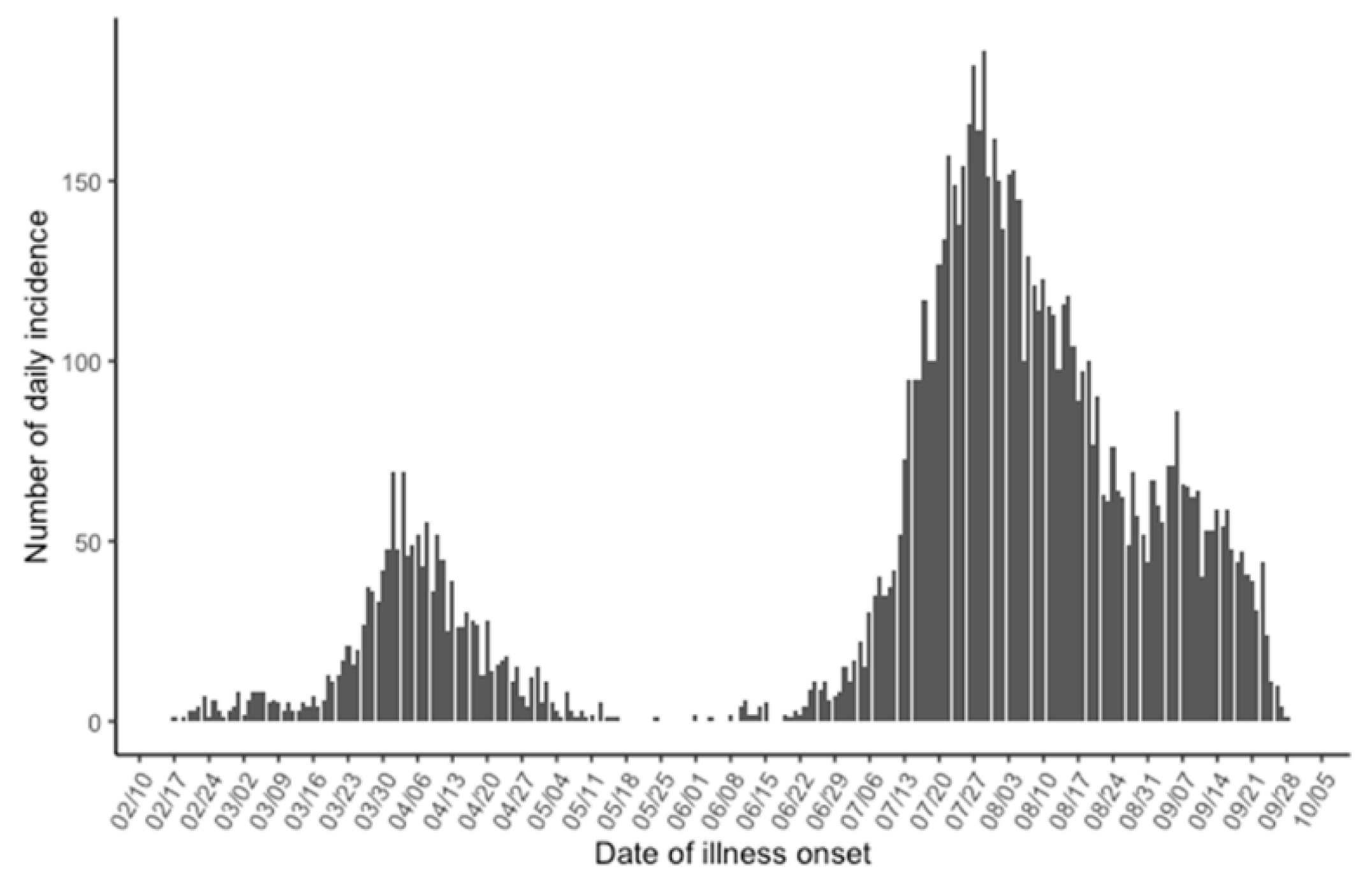
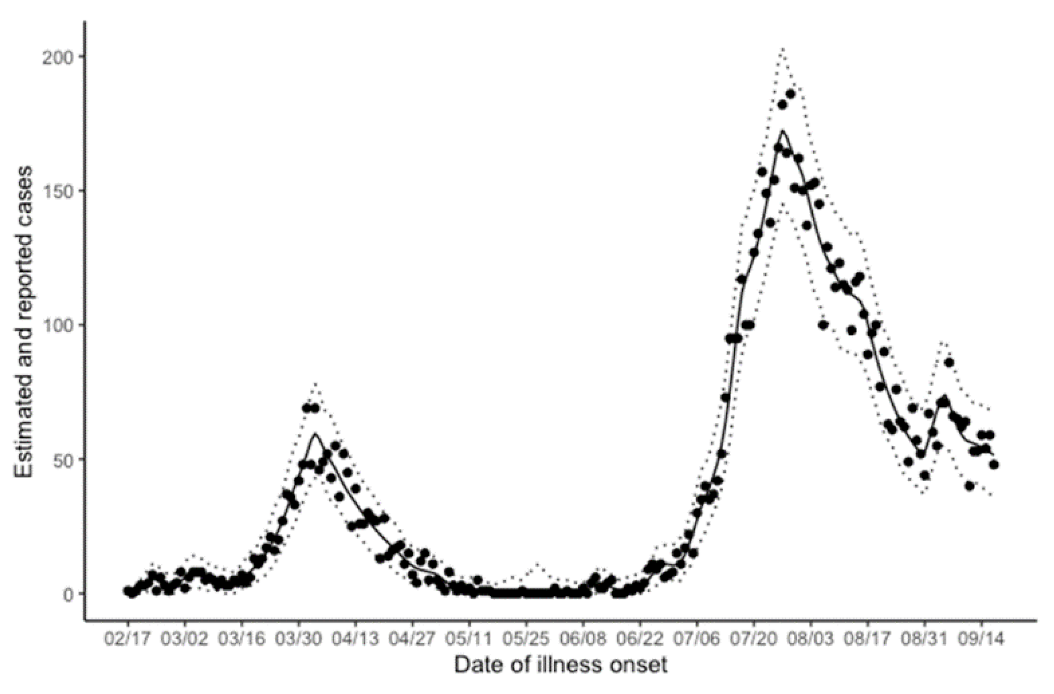
2.1. Epidemiological Data
2.2. Public Health Intervention Implementation
2.3. Model Descriptions
2.4. Model Comparison and Sensitivity Analysis
2.5. Data Sharing Statement
3. Results
4. Discussion
Supplementary Materials
Author Contributions
Funding
Institutional Review Board Statement
Informed Consent Statement
Data Availability Statement
Conflicts of Interest
Appendix A

| Model | Day 31 | Day 39 | Day 43 | Day 46 | p-Value | |
|---|---|---|---|---|---|---|
| 1 | 0 | 1 | 1 | 1 | 0.24059 | |
| 2 | 1 | 0 | 1 | 1 | 0.76617 | |
| 3 | 1 | 1 | 0 | 1 | 0.67850 | |
| 4 | 1 | 1 | 1 | 0 | 0.15528 | |
| 5 | 0 | 0 | 1 | 1 | 0.36975 | |
| 6 | 0 | 1 | 0 | 1 | 0.40291 | |
| 7 | 0 | 1 | 1 | 0 | 0.00000 | * |
| 8 | 1 | 0 | 0 | 1 | 0.00000 | * |
| 9 | 1 | 0 | 1 | 0 | 0.00000 | * |
| 10 | 1 | 1 | 0 | 0 | 0.00000 | * |
| 11 | 0 | 0 | 0 | 1 | 0.00000 | * |
| 12 | 0 | 0 | 1 | 0 | 0.00000 | * |
| 13 | 0 | 1 | 0 | 0 | 0.00000 | * |
| 14 | 1 | 0 | 0 | 0 | 0.00000 | * |
| 15 | 0 | 0 | 0 | 0 | 0.00059 | * |
| joinpoint | N | N | Y | Y |
| Model | Day 162 | Day 165 | p-Value |
|---|---|---|---|
| 1 | 0 | 1 | 0.45741 |
| 2 | 1 | 0 | 0.66792 |
| 3 | 0 | 0 | 0.86868 |
| joinpoint | N | N |


References
- Hayashi, K.; Kayano, T.; Sorano, S.; Nishiura, H. Hospital caseload demand in the presence of interventions during the covid-19 pandemic: A modeling study. J. Clin. Med. 2020, 9, 3065. [Google Scholar] [CrossRef] [PubMed]
- Li, R.; Rivers, C.; Tan, Q.; Murray, M.B.; Toner, E.; Lipsitch, M. Estimated demand for US hospital inpatient and intensive care unit beds for patients with Covid-19 based on comparisons with Wuhan and Guangzhou, China. JAMA Netw. Open 2020, 3, e208297. [Google Scholar] [CrossRef] [PubMed]
- Flaxman, S.; Mishra, S.; Gandy, A.; Unwin, H.J.T.; Mellan, T.A.; Coupland, H.; Whittaker, C.; Zhu, H.; Berah, T.; Eaton, J.W.; et al. Estimating the effects of non-pharmaceutical interventions on COVID-19 in Europe. Nature 2020, 584, 257–261. [Google Scholar] [CrossRef] [PubMed]
- Pan, A.; Liu, L.; Wang, C.; Guo, H.; Hao, X.; Wang, Q.; Huang, J.; He, N.; Yu, H.; Lin, X.; et al. Association of public health interventions with the epidemiology of the Covid-19 outbreak in Wuhan, China. JAMA J. Am. Med. Assoc. 2020, 323, 1915–1923. [Google Scholar] [CrossRef] [PubMed]
- Abbott, S.; Hellewell, J.; Thompson, R.N.; Sherratt, K.; Gibbs, H.P.; Bosse, N.I.; Munday, J.D.; Meakin, S.; Doughty, E.L.; Chun, J.Y.; et al. Estimating the time-varying reproduction number of SARS-CoV-2 using national and subnational case counts. Wellcome Open Res. 2020, 5, 112. [Google Scholar] [CrossRef]
- Kucharski, A.J.; Russell, T.W.; Diamond, C.; Liu, Y.; Edmunds, J.; Funk, S.; Eggo, R.M.; Sun, F.; Jit, M.; Munday, J.D.; et al. Early dynamics of transmission and control of COVID-19: A mathematical modelling study. Lancet Infect. Dis. 2020, 20, 553–558. [Google Scholar] [CrossRef]
- Tariq, A.; Lee, Y.; Roosa, K.; Blumberg, S.; Yan, P.; Ma, S.; Chowell, G. Real-time monitoring the transmission potential of COVID-19 in Singapore, March 2020. BMC Med. 2020, 18, 166. [Google Scholar] [CrossRef]
- Caicedo-Ochoa, Y.; Rebellón-Sánchez, D.E.; Peñaloza-Rallón, M.; Cortés-Motta, H.F.; Méndez-Fandiño, Y.R. Effective Reproductive Number estimation for initial stage of COVID-19 pandemic in Latin American Countries. Int. J. Infect. Dis. 2020, 95, 316–318. [Google Scholar] [CrossRef]
- Wallinga, J.; Teunis, P. Different epidemic curves for severe acute respiratory syndrome reveal similar impacts of control measures. Am. J. Epidemiol. 2004, 160, 509–516. [Google Scholar] [CrossRef]
- Cori, A.; Ferguson, N.M.; Fraser, C.; Cauchemez, S. A new framework and software to estimate time-varying reproduction numbers during epidemics. Am. J. Epidemiol. 2013, 178, 1505–1512. [Google Scholar] [CrossRef]
- Scire, J.; Nadeau, S.; Vaughan, T.; Brupbacher, G.; Fuchs, S.; Sommer, J.; Koch, K.N.; Misteli, R.; Mundorff, L.; Götz, T.; et al. Reproductive number of the COVID-19 epidemic in Switzerland with a focus on the Cantons of Basel-Stadt and Basel-Landschaft. Swiss Med. Wkly. 2020, 150, w20271. [Google Scholar] [CrossRef]
- Ryu, S.; Ali, S.T.; Jang, C.; Kim, B.; Cowling, B.J. Effect of nonpharmaceutical interventions on transmission of severe acute respiratory syndrome Coronavirus 2, South Korea, 2020. Emerg. Infect. Dis. 2020, 26, 2406–2410. [Google Scholar] [CrossRef]
- Kuniya, T. Evaluation of the effect of the state of emergency for the first wave of COVID-19 in Japan. Infect. Dis. Model. 2020, 5, 580–587. [Google Scholar] [CrossRef] [PubMed]
- Gostic, K.M.; Mcgough, L.; Baskerville, E.B.; Abbott, S.; Joshi, K.; Tedijanto, C.; Kahn, R.; Niehus, R.; Hay, J.; De Salazar, P.M.; et al. Practical considerations for measuring the effective reproductive number, R t. medRxiv 2020. [Google Scholar] [CrossRef]
- Nishiura, H.; Chowell, G. The effective reproduction number as a prelude to statistical estimation of time-dependent epidemic trends. In Mathematical and Statistical Estimation Approaches in Epidemiology; Springer: New York, NY, USA, 2009; pp. 103–121. ISBN 9789048123124. [Google Scholar] [CrossRef]
- Wallinga, J.; Lipsitch, M. How generation intervals shape the relationship between growth rates and reproductive numbers. Proc. R. Soc. B Biol. Sci. 2007, 274, 599–604. [Google Scholar] [CrossRef] [PubMed]
- Nishiura, H.; Linton, N.M.; Akhmetzhanov, A.R. Serial interval of novel coronavirus (COVID-19) infections. Int. J. Infect. Dis. 2020, 93, 284–286. [Google Scholar] [CrossRef]
- He, X.; Lau, E.H.Y.; Wu, P.; Deng, X.; Wang, J.; Hao, X.; Lau, Y.C.; Wong, J.Y.; Guan, Y.; Tan, X.; et al. Temporal dynamics in viral shedding and transmissibility of COVID-19. Nat. Med. 2020, 26, 672–675. [Google Scholar] [CrossRef]
- Liu, Y.; Funk, S.; Flasche, S.; Jit, M.; Bosse, N.I.; Gimma, A.; Klepac, P.; Russell, T.W.; Sun, F.; Rosello, A.; et al. The contribution of pre-symptomatic infection to the transmission dynamics of COVID-2019. Wellcome Open Res. 2020. [Google Scholar] [CrossRef]
- Yang, L.; Dai, J.; Zhao, J.; Wang, Y.; Deng, P.; Wang, J. Estimation of incubation period and serial interval of COVID-19: Analysis of 178 cases and 131 transmission chains in Hubei province, China. Epidemiol. Infect. 2020, 148, e117. [Google Scholar] [CrossRef]
- Li, Q.; Guan, X.; Wu, P.; Wang, X.; Zhou, L.; Tong, Y.; Ren, R.; Leung, K.S.M.; Lau, E.H.Y.; Wong, J.Y.; et al. Early transmission dynamics in Wuhan, China, of novel coronavirus-infected pneumonia. N. Engl. J. Med. 2020, 382, 1199–1207. [Google Scholar] [CrossRef] [PubMed]
- Linton, N.; Kobayashi, T.; Yang, Y.; Hayashi, K.; Akhmetzhanov, A.; Jung, S.; Yuan, B.; Kinoshita, R.; Nishiura, H. Incubation period and other epidemiological characteristics of 2019 novel Coronavirus infections with right truncation: A statistical analysis of publicly available case data. J. Clin. Med. 2020, 9, 538. [Google Scholar] [CrossRef]
- Nishiura, H.; Chowell, G. Early transmission dynamics of Ebola virus disease (evd), West Africa, March to August 2014. Eurosurveillance 2014, 19, 1–6. [Google Scholar] [CrossRef]
- Ganyani, T.; Kremer, C.; Chen, D.; Torneri, A.; Faes, C.; Wallinga, J.; Hens, N. Estimating the generation interval for coronavirus disease (COVID-19) based on symptom onset data, March 2020. Eurosurveillance 2020. [Google Scholar] [CrossRef]
- Becker, N.G.; Watson, L.F.; Carlin, J.B. A method of non-parametric back-projection and its application to aids data. Stat. Med. 1991, 10, 1527–1542. [Google Scholar] [CrossRef]
- Joinpoint Regression Program; Version 4.8.0; Statistical Methodology and Applications Branch, Surveillance Research Program; National Cancer Institute: Bethesda, MD, USA, 1 April 2020.
- Petermann, M.; Wyler, D. A pitfall in estimating the e ective reproductive number Rt for COVID-19. Swiss Med. Wkly. 2020, 150, w20307. [Google Scholar] [CrossRef]
- Lipsitch, M.; Joshi, K.; Cobey, S.E. Comment on Pan A, Liu L, Wang C; et al. Association of Public Health Interventions with the epidemiology of the COVID-19 outbreak in Wuhan, China. JAMA J. Am. Med. Assoc. 2020, 323, 1915–1923. [Google Scholar] [CrossRef]
- Kendall, M.; Milsom, L.; Abeler-Doerner, L.; Wymant, C.; Ferretti, L.; Briers, M.; Holmes, C.; Bonsall, D.; Abeler, J.; Fraser, C. Epidemiological changes on the Isle of Wight after the launch of the NHS Test and Trace programme: A preliminary analysis. Lancet Digit. Health 2020, 2, e658–e666. [Google Scholar] [CrossRef]
- Davies, N.G.; Klepac, P.; Liu, Y.; Prem, K.; Jit, M.; Pearson, C.A.B.; Quilty, B.J.; Kucharski, A.J.; Gibbs, H.; Clifford, S.; et al. Age-dependent effects in the transmission and control of COVID-19 epidemics. Nat. Med. 2020, 26, 1205–1211. [Google Scholar] [CrossRef]
- Ayoub, H.H.; Chemaitelly, H.; Seedat, S.; Mumtaz, G.R.; Makhoul, M.; Abu-Raddad, L.J. Age could be driving variable SARS-CoV-2 epidemic trajectories worldwide. PLoS ONE 2020, 15, e0237959. [Google Scholar] [CrossRef]
- Ali, S.T.; Wang, L.; Lau, E.H.Y.; Xu, X.K.; Du, Z.; Wu, Y.; Leung, G.M.; Cowling, B.J. Serial interval of SARS-CoV-2 was shortened over time by nonpharmaceutical interventions. Science 2020, 369, 1106–1109. [Google Scholar] [CrossRef]
- Chan, Y.H.; Nishiura, H. Estimating the protective effect of case isolation with transmission tree reconstruction during the Ebola outbreak in Nigeria, 2014. J. R. Soc. Interface 2020, 17, 20200498. [Google Scholar] [CrossRef] [PubMed]
- Rao, A.S.R.; Krantz, S.G.; Bonsall, M.B.; Kurien, T.; Byrareddy, S.N.; Swanson, D.A.; Bhat, R.; Sudhakar, K. How relevant is the basic reproductive number computed during covid-19, especially during lockdowns? Infect. Control Hosp. Epidemiol. 2020, in press. [Google Scholar] [CrossRef]


| Calendar Date | Analysis Date | Description |
|---|---|---|
| First wave | ||
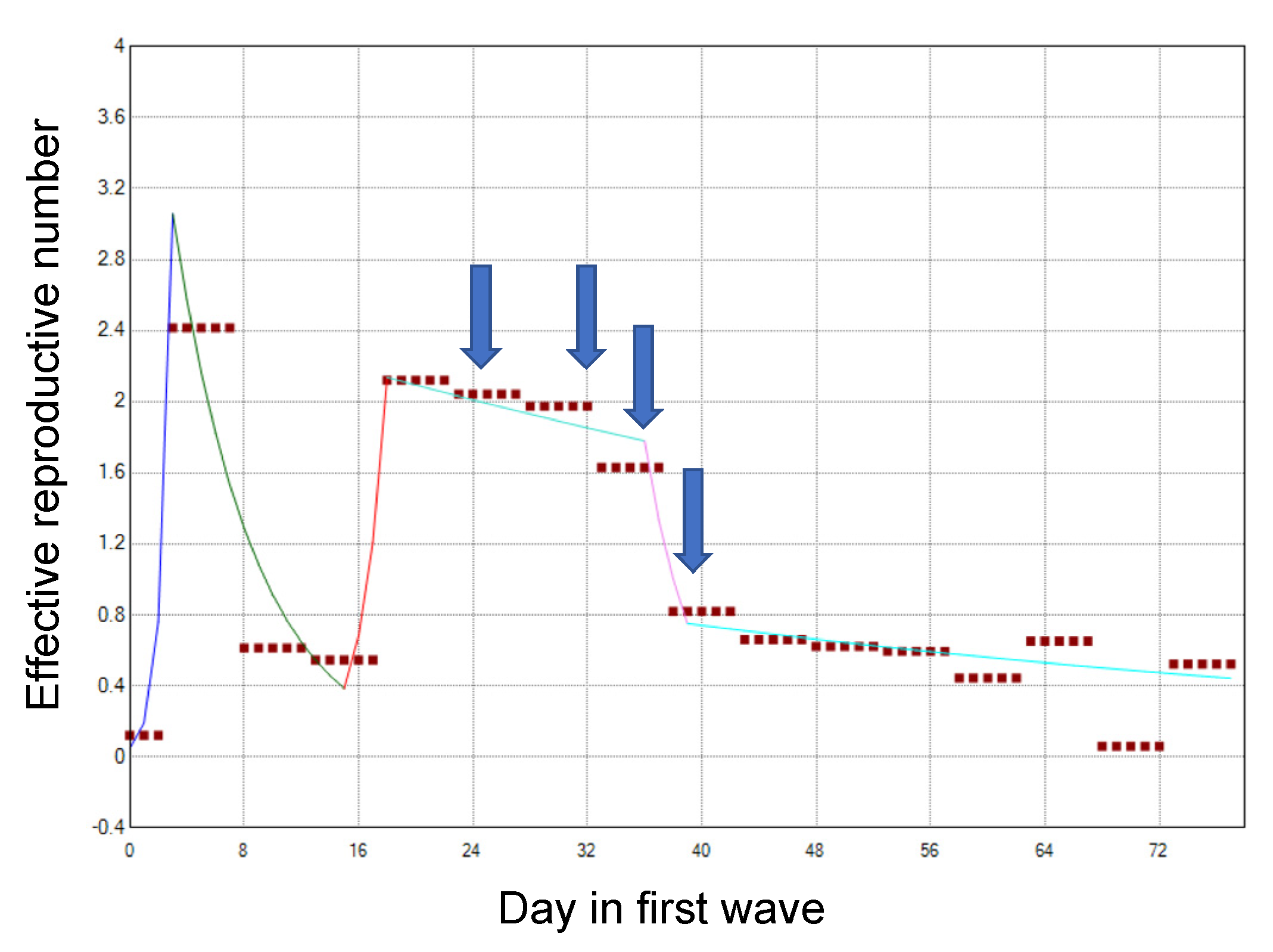
| 17 February | Day 0 | The index case developed illness. |
| 1 March | Day 13 | The governor requested the government to dispatch an emergency operations center team (“cluster busters team”). |
| 19 March | Day 31 | Voluntary restrictions on crossing the border of Osaka (especially between Osaka and Hyogo) were requested. |
| 27 March | Day 39 | Voluntary restrictions on weekend outings were requested. |
| 31 March | Day 43 | Voluntary restrictions on eating at restaurants operating at nighttime were requested. |
| 3 April | Day 46 | Voluntary restrictions on weekend outings were requested for the second time. |
| 7 April | Day 50 | A state of emergency was declared by the Prime Minister. |
| 5 May | Day 78 | The original classification of the epidemiological situation (the “Osaka model”) was announced. |
| 21 May | Day 94 | Osaka was released from the state of emergency. |
| Second wave | ||
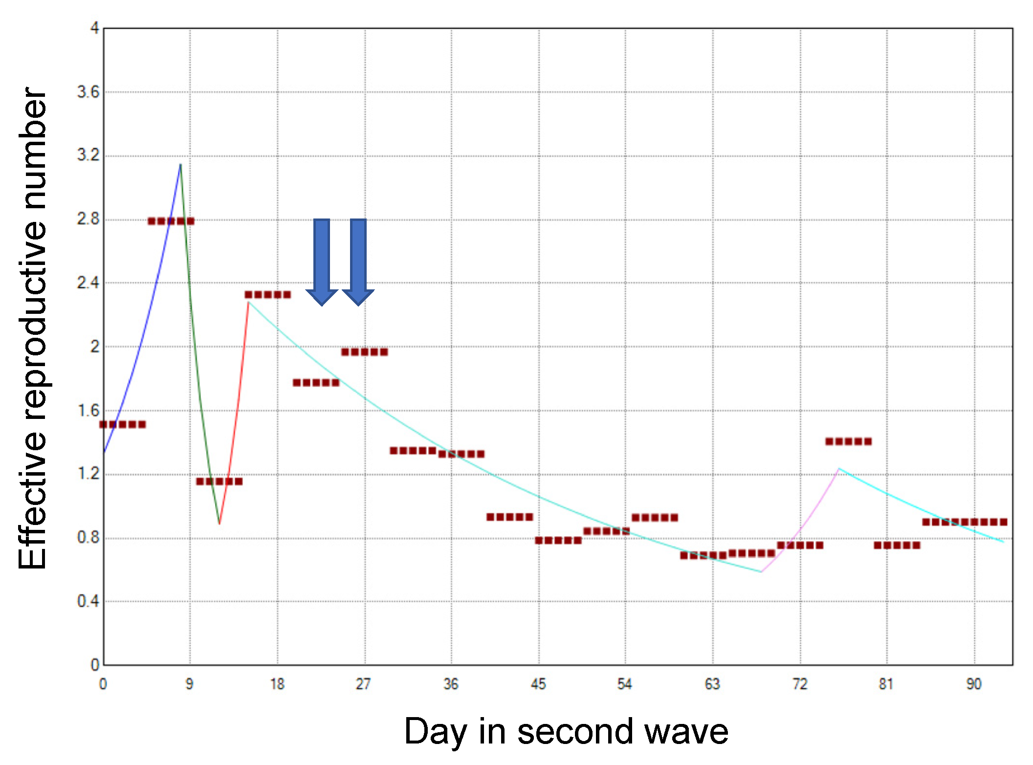
| 12 July | Day 146 | A first alert was issued according to the Osaka model. |
| 28 July | Day 162 | Voluntary restrictions on social events involving the consumption of alcohol by more than four persons were requested. |
| 31 July | Day 165 | Restaurants and bars in specific districts of Osaka city were requested to voluntarily close. |
| 21 August | Day 186 | Restaurants and bars were allowed to open. |
| 31 August | Day 196 | Restrictions on social events involving the consumption of alcohol by more than four persons were lifted. |
Publisher’s Note: MDPI stays neutral with regard to jurisdictional claims in published maps and institutional affiliations. |
© 2021 by the authors. Licensee MDPI, Basel, Switzerland. This article is an open access article distributed under the terms and conditions of the Creative Commons Attribution (CC BY) license (http://creativecommons.org/licenses/by/4.0/).
Share and Cite
Nakajo, K.; Nishiura, H. Assessing Interventions against Coronavirus Disease 2019 (COVID-19) in Osaka, Japan: A Modeling Study. J. Clin. Med. 2021, 10, 1256. https://doi.org/10.3390/jcm10061256
Nakajo K, Nishiura H. Assessing Interventions against Coronavirus Disease 2019 (COVID-19) in Osaka, Japan: A Modeling Study. Journal of Clinical Medicine. 2021; 10(6):1256. https://doi.org/10.3390/jcm10061256
Chicago/Turabian StyleNakajo, Ko, and Hiroshi Nishiura. 2021. "Assessing Interventions against Coronavirus Disease 2019 (COVID-19) in Osaka, Japan: A Modeling Study" Journal of Clinical Medicine 10, no. 6: 1256. https://doi.org/10.3390/jcm10061256
APA StyleNakajo, K., & Nishiura, H. (2021). Assessing Interventions against Coronavirus Disease 2019 (COVID-19) in Osaka, Japan: A Modeling Study. Journal of Clinical Medicine, 10(6), 1256. https://doi.org/10.3390/jcm10061256