Membrane BioReactor (MBR) Activated Sludge Surrogate Alternatives Carboxymethyl Cellulose and Xanthan Gum: A Statistical Analysis and Review
Abstract
:1. Introduction
2. Activated Sludge for Membrane Bioreactos and Applications of Non-Newtonian Liquids (CMC and XG) in the Literature
3. Comparison of Rheological Parameters
3.1. Proposed Assessment: Seeking for Insights and Trends
3.2. CMC Regression Results
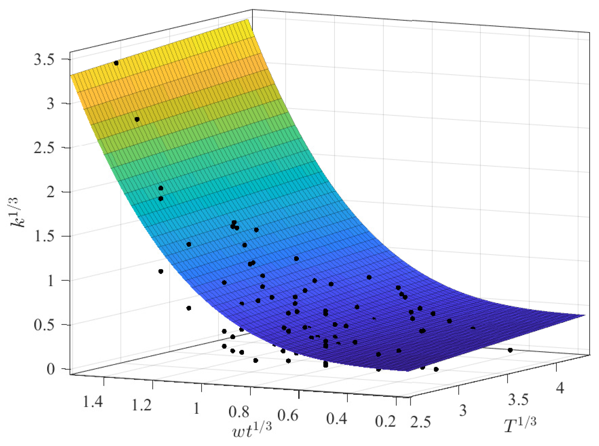
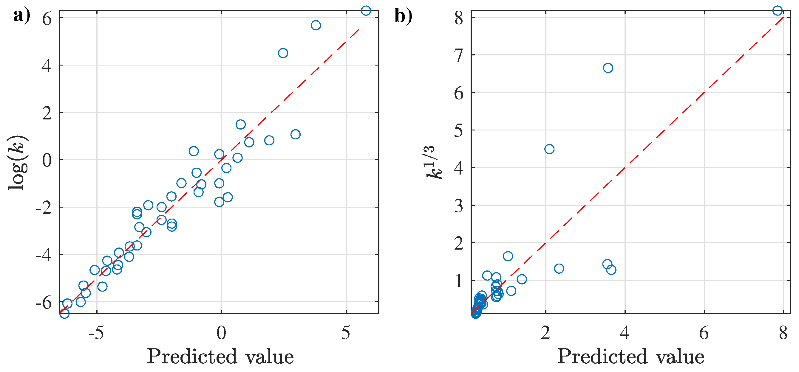
3.2.1. Prediction of k as a Function of and T
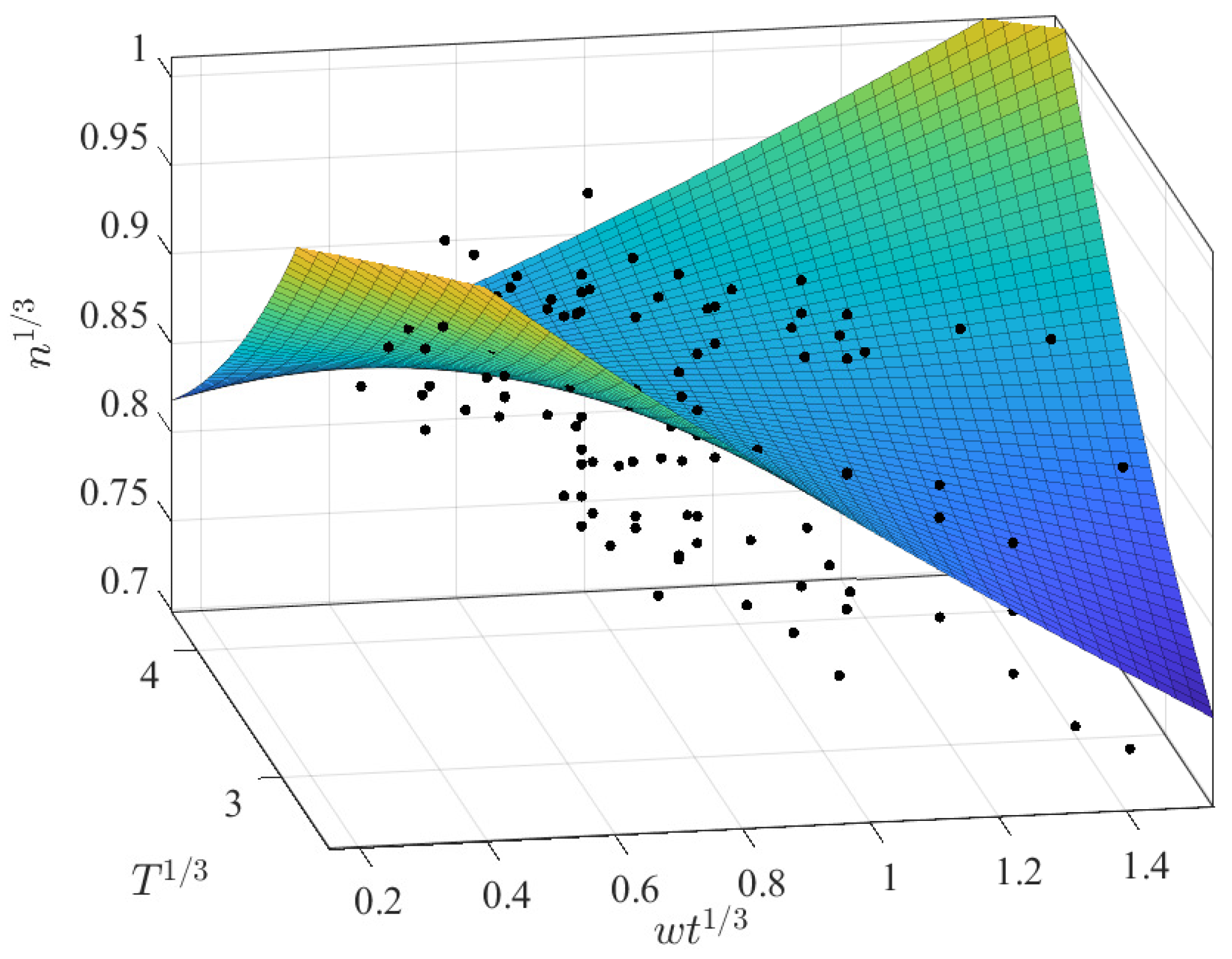
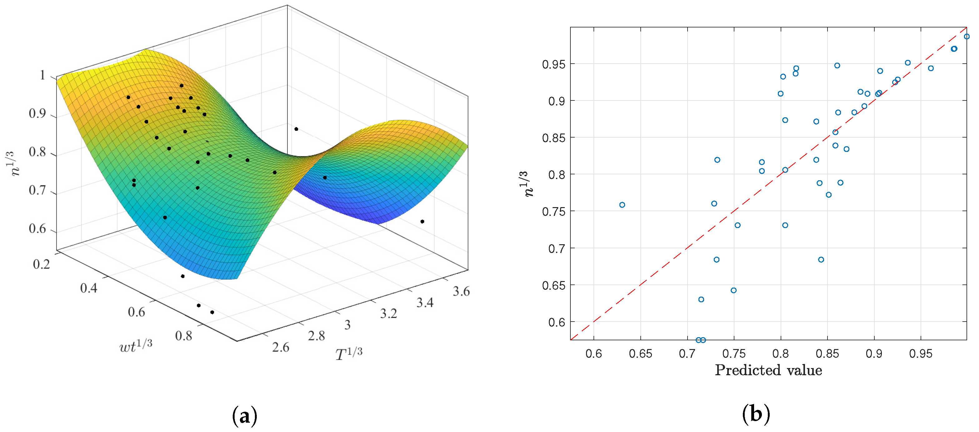
3.2.2. Prediction of n as a Function of and T
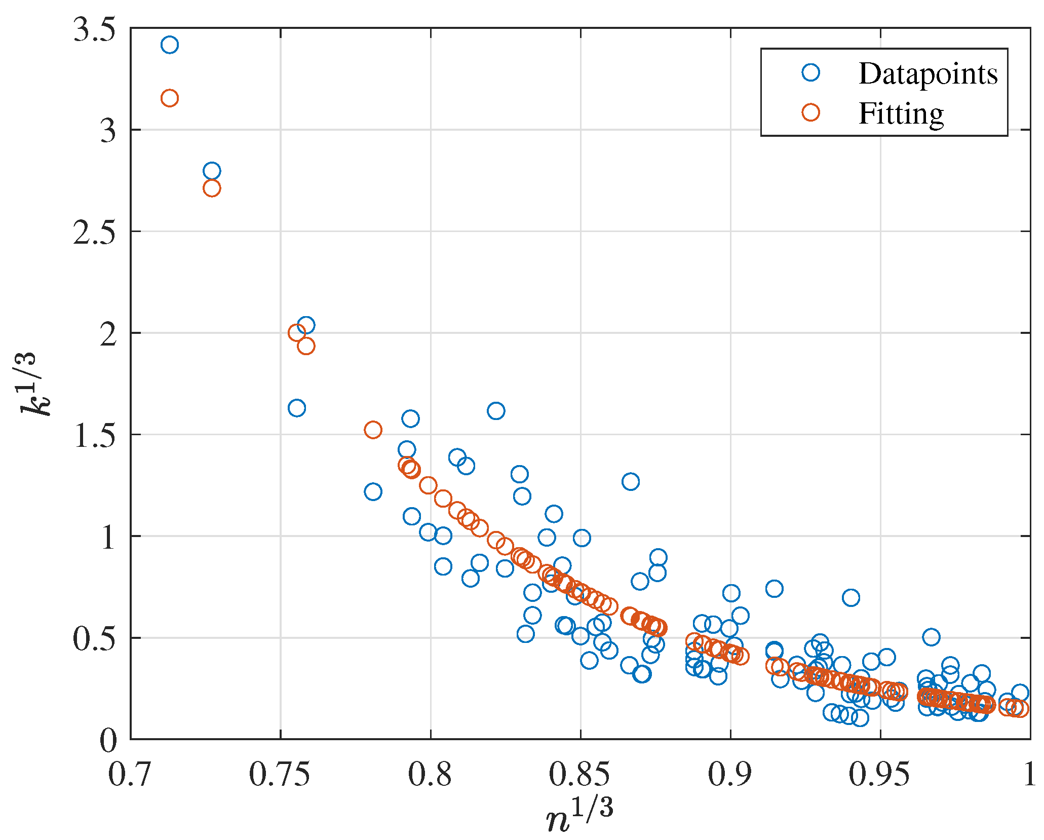
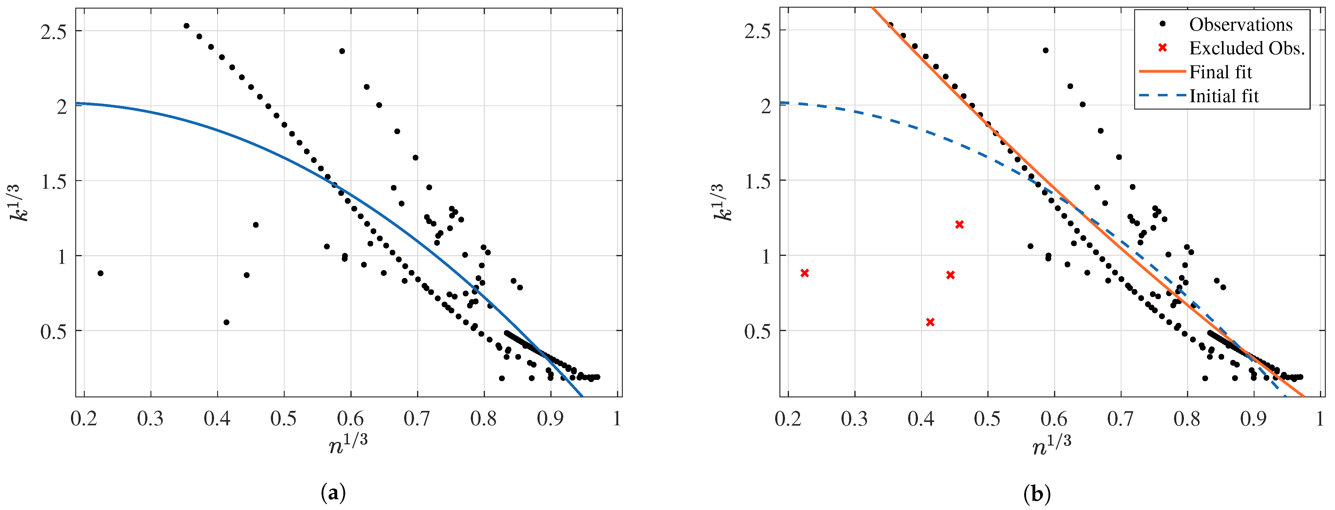
3.2.3. Prediction of k as a Function of n
3.3. XG Regression Results
3.3.1. Prediction of k as a Function of and T
3.3.2. Prediction of n as a Function of and T
3.3.3. Prediction of k as a Function of n
3.4. AS Regression Results
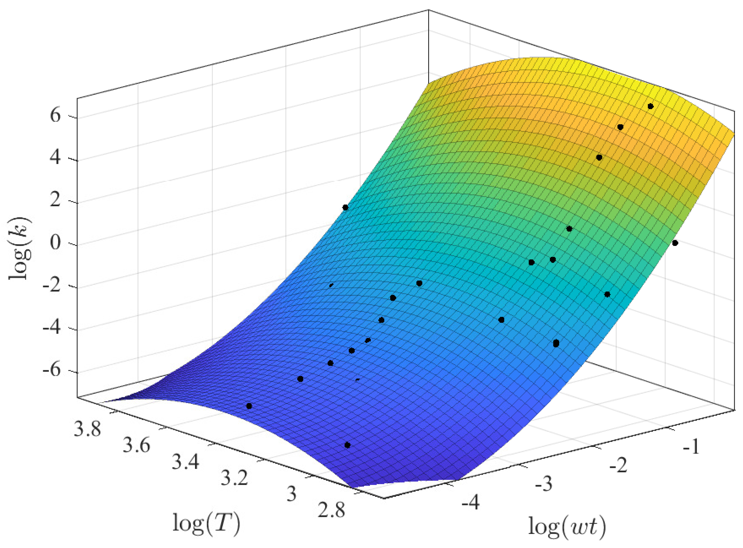
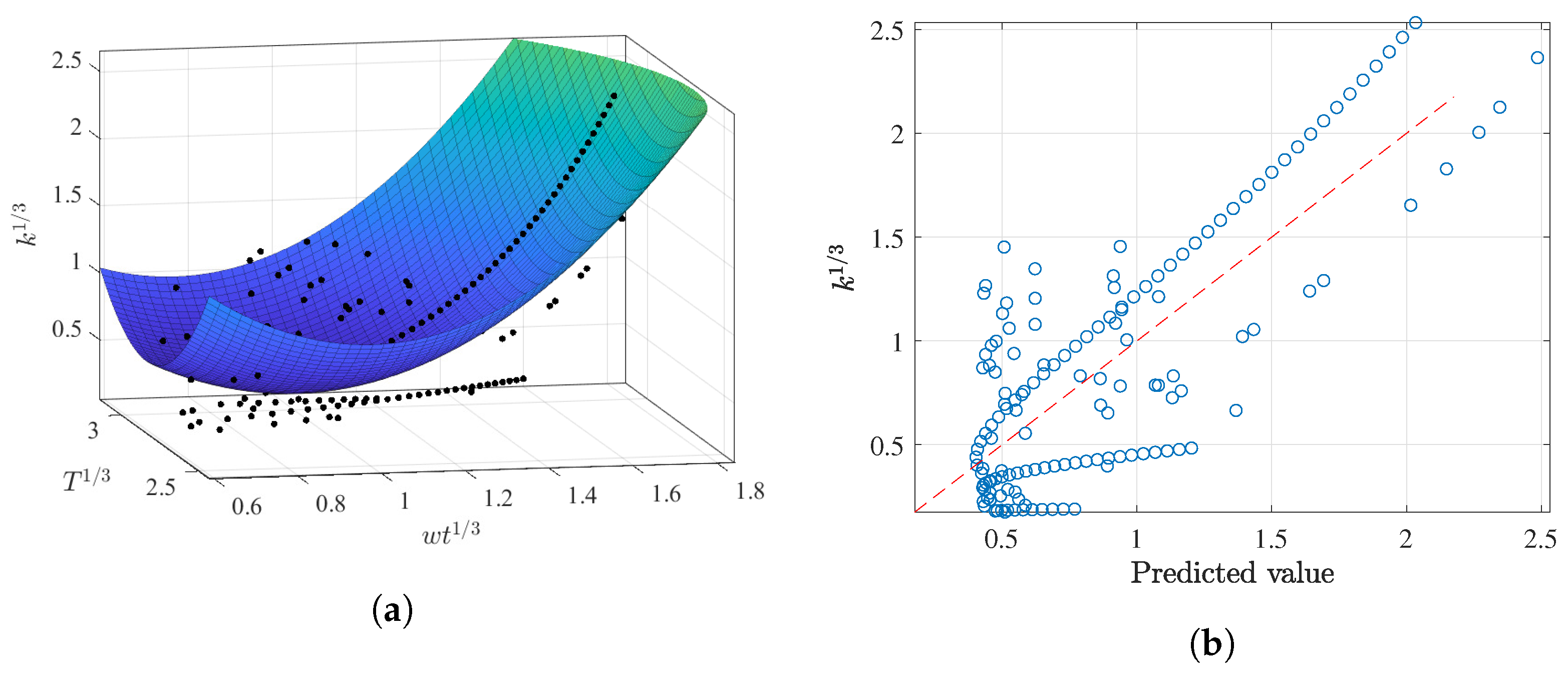
3.4.1. Prediction of k as a Function of and T
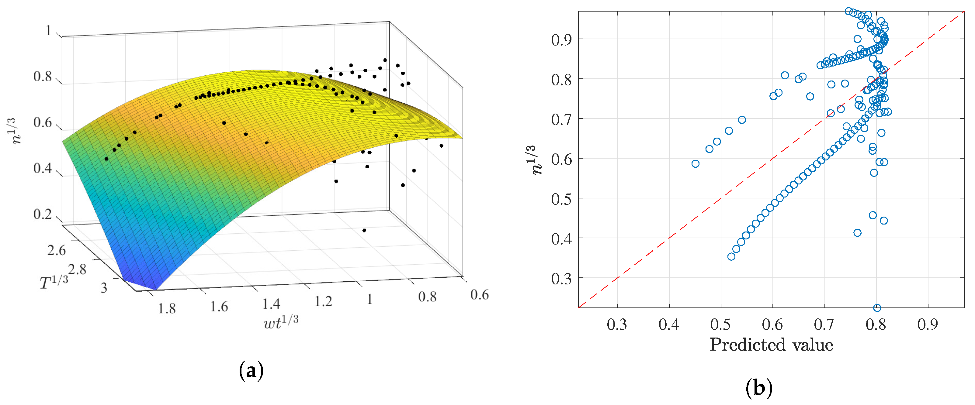
3.4.2. Prediction of n as a Function of and T
3.4.3. Prediction of k as a Function of n
4. Conclusions
- Research using these different compounds does not focus on the determination of rheological properties, except for the work of Benchabane and Bekkour [90] and that of Ghannam and Esmail [94]. All other studies used the non-Newtonian compounds to determine the behaviors of specific systems. Therefore, no attention was paid to the procedure by which the viscosity measurements were obtained.
- Different rheometers/geometries were used for the viscosity measurements (i.e., concentric cylinders, cone-and-plates, double gaps, and tubular), which produced different results.
- Various experimental protocols were implemented.
- The chemicals used were from different chemical manufacturers.
Author Contributions
Funding
Institutional Review Board Statement
Informed Consent Statement
Data Availability Statement
Conflicts of Interest
Abbreviations
| AS | Activated Sludge |
| CAS | Conventional Activated Sludge |
| CFD | Computational Fluid Dynamics |
| CMC | Carboxymethyl Cellulose |
| DG-CC | Double Gap Concentric Cylinder geometry |
| ERT | Electrical Resistance Tomography |
| MBR | Membrane Bioreactors |
| MLSS | Mixed Liquor Suspended Solids |
| PEPT | Positron Emission Particle Tracking |
| PIV | Particle Imaging Velocimetry |
| PSD | Particle Size Distribution |
| PST | Pulse Shadow Technique |
| TSS | Total Suspended Solids |
| WWT | Wastewater treatment |
| XG | Xanthan Gum |
References
- Westra, J.G. Rheology of carboxymethyl cellulose with xanthan gum properties. Macromolecules 1989, 22, 367–370. [Google Scholar] [CrossRef]
- Slatter, P. The rheological characterisation of sludges. Water Sci. Technol. 1997, 36, 9–18. [Google Scholar] [CrossRef]
- Bailey, W.; Weir, I. Investigation of methods for direct rheological model parameter estimation. J. Pet. Sci. Eng. 1998, 21, 1–13. [Google Scholar] [CrossRef]
- Carezzato, A.; Alcantara, M.; Telis-Romero, J.; Tadini, C.; Gut, J. Non-Newtonian Heat Transfer on a Plate Heat Exchanger with Generalized Configurations. Chem. Eng. Technol. 2007, 30, 21–26. [Google Scholar] [CrossRef]
- Linstrom, P.J.; Mallard, W.G. NIST Chemistry WebBook. In Technical Report, NIST Standard Reference; Database Number 69; NIST: Gaithersburg, MD, USA, 2009. [Google Scholar]
- Brannock, M.; Wang, Y.; Leslie, G. Mixing characterisation of full-scale membrane bioreactors: CFD modelling with experimental validation. Water Res. 2010, 44, 3181–3191. [Google Scholar] [CrossRef] [PubMed]
- Defrance, L.; Jaffrin, M.; Gupta, B.; Paullier, P.; Geaugey, V. Contribution of various constituents of activated sludge to membrane bioreactor fouling. Bioresour. Technol. 2000, 73, 105–112. [Google Scholar] [CrossRef]
- Xia, M.; Wang, Z.; Wu, Z.; Wang, X.; Zhou, Z.; Lu, J. Simulation and assessment of sludge concentration and rheology in the process of waste activated sludge treatment. J. Environ. Sci. 2009, 21, 1639–1645. [Google Scholar] [CrossRef]
- Zhao, W.T.; Huang, X.; Lee, D.J.; Wang, X.H.; Shen, Y.X. Use of submerged anaerobic–anoxic–oxic membrane bioreactor to treat highly toxic coke wastewater with complete sludge retention. J. Membr. Sci. 2009, 330, 57–64. [Google Scholar] [CrossRef]
- Rosenberger, S.; Kubin, K.; Kraume, M. Rheology of Activated Sludge in Membrane Bioreactors. Eng. Life Sci. 2002, 2, 269–275. [Google Scholar] [CrossRef]
- Hasar, H.; Kinaci, C.; Ünlü, A.; Toǧrul, H.; Ipek, U. Rheological properties of activated sludge in a sMBR. Biochem. Eng. J. 2004, 20, 1–6. [Google Scholar] [CrossRef]
- Garakani, A.K.; Mostoufi, N.; Sadeghi, F.; Fatourechi, H.; Sarrafzadeh, M.; Mehrnia, M. Comparison between Different Models for Rheological Characterization of Activated Sludge. Iran. J. Environ. Health Sci. Eng. 2011, 8, 255–264. [Google Scholar]
- Yang, F.; Bick, A.; Shandalov, S.; Brenner, A.; Oron, G. Yield stress and rheological characteristics of activated sludge in an airlift membrane bioreactor. J. Membr. Sci. 2009, 334, 83–90. [Google Scholar] [CrossRef]
- Laera, G.; Giordano, C.; Pollice, A.; Saturno, D.; Mininni, G. Membrane bioreactor sludge rheology at different solid retention times. Water Res. 2007, 41, 4197–4203. [Google Scholar] [CrossRef]
- Pollice, A.; Giordano, C.; Laera, G.; Saturno, D.; Mininni, G. Physical characteristics of the sludge in a complete retention membrane bioreactor. Water Res. 2007, 41, 1832–1840. [Google Scholar] [CrossRef] [PubMed]
- Pollice, A.; Giordano, C.; Laera, G.; Saturno, D.; Mininni, G. Rheology of Sludge in a Complete Retention Membrane Bioreactor. Environ. Technol. 2006, 27, 723–732. [Google Scholar] [CrossRef]
- Seyssiecq, I.; Ferrasse, J.H.; Roche, N. State-of-the-art: Rheological characterisation of wastewater treatment sludge. Biochem. Eng. J. 2003, 16, 41–56. [Google Scholar] [CrossRef]
- Mori, M.; Seyssiecq, I.; Roche, N. Rheological measurements of sewage sludge for various solids concentrations and geometry. Process. Biochem. 2006, 41, 1656–1662. [Google Scholar] [CrossRef]
- Liu, X.; Wang, Y.; Waite, T.; Leslie, G. Numerical simulation of bubble induced shear in membrane bioreactors: Effects of mixed liquor rheology and membrane configuration. Water Res. 2015, 75, 131–145. [Google Scholar] [CrossRef]
- Radaei, E.; Liu, X.; Tng, K.; Wang, Y.; Trujillo, F.; Leslie, G. Insights on pulsed bubble control of membrane fouling: Effect of bubble size and frequency. J. Membr. Sci. 2018, 554, 59–70. [Google Scholar] [CrossRef]
- Duran, C.; Fayolle, Y.; Pechaud, Y.; Cockx, A.; Gillot, S. Impact of suspended solids on the activated sludge non-newtonian behaviour and on oxygen transfer in a bubble column. Chem. Eng. Sci. 2016, 141, 154–165. [Google Scholar] [CrossRef]
- Moreau, A.; Ratkovich, N.; Nopens, I.; van der Graaf, J. The (in)significance of apparent viscosity in full-scale municipal membrane bioreactors. J. Membr. Sci. 2009, 340, 249–256. [Google Scholar] [CrossRef]
- Lopez, J.; Moreau, A.; Gil, J.; van der Graaf, J.; van Lier, J.; Ratkovich, N. MBR activated sludge viscosity measurement using the Delft filtration characterization method. J. Water Process. Eng. 2015, 5, 35–41. [Google Scholar] [CrossRef]
- Grutzmacher, D. Are you Using the Right Tank Design for Your Industrial Mixing Application? (Part 1). 2016. Available online: https://proquipinc.com/tank-design-industrial-mixing-application/ (accessed on 1 June 2022).
- Pugliesi, D. Representation of a Bubble Column Reactor. 2012. Available online: https://en.wikipedia.org/wiki/Bubble_column_reactor#/media/File:Bubble_column.svg (accessed on 1 June 2022).
- Amaya-Gómez, R.; López, J.; Pineda, H.; Urbano-Caguasango, D.; Pinilla, J.; Ratkovich, N.; Muñoz, F. Probabilistic approach of a flow pattern map for horizontal, vertical, and inclined pipes. Oil Gas Sci. Technol.-Rev. Ifp Energies Nouv. 2019, 74, 67. [Google Scholar] [CrossRef]
- Miura, H.; Takahashi, T.; Ichikawa, J.; Kawase, Y. Bed expansion in liquid–solid two-phase fluidized beds with Newtonian and non-Newtonian fluids over the wide range of Reynolds numbers. Powder Technol. 2001, 117, 239–246. [Google Scholar] [CrossRef]
- Iliuta, I.; Aydin, B.; Larachi, F. Onset of pulsing in trickle beds with non-Newtonian liquids at elevated temperature and pressure—Modeling and experimental verification. Chem. Eng. Sci. 2006, 61, 526–537. [Google Scholar] [CrossRef]
- Shimizu, K.; Minekawa, K.; Hirose, T.; Kawase, Y. Drop breakage in stirred tanks with Newtonian and non-Newtonian fluid systems. Chem. Eng. J. 1999, 72, 117–124. [Google Scholar] [CrossRef]
- García-Ochoa, F.; Gómez, E. Mass transfer coefficient in stirred tank reactors for xanthan gum solutions. Biochem. Eng. J. 1998, 1, 1–10. [Google Scholar] [CrossRef]
- Burru, I.; Briens, C. Particle—Liquid mass transfer in three-phase fluidized beds: Part II. Non-Newtonian liquids. Powder Technol. 1991, 68, 255–261. [Google Scholar] [CrossRef]
- Abukhalifeh, H.; Fayed, M.; Dhib, R. Hydrodynamics of TBC with non-Newtonian liquids: Liquid holdup. Chem. Eng. Process. Process. Intensif. 2009, 48, 1222–1228. [Google Scholar] [CrossRef]
- Lali, A.; Khare, A.; Joshi, J.; Nigam, K. Behaviour of solid particles in viscous non-newtonian solutions: Settling velocity, wall effects and bed expansion in solid-liquid fluidized beds. Powder Technol. 1989, 57, 39–50. [Google Scholar] [CrossRef]
- Miura, H.; Kawase, Y. Hydrodynamics and mass transfer in three-phase fluidized beds with non-Newtonian fluids. Chem. Eng. Sci. 1997, 52, 4095–4104. [Google Scholar] [CrossRef]
- Miura, H.; Kawase, Y. Minimum liquid fluidization velocity in two- and three-phase fluidized beds with non-Newtonian fluids. Powder Technol. 1998, 97, 124–128. [Google Scholar] [CrossRef]
- Aydin, B.; Larachi, F. Trickle bed hydrodynamics and flow regime transition at elevated temperature for a Newtonian and a non-Newtonian liquid. Chem. Eng. Sci. 2005, 60, 6687–6701. [Google Scholar] [CrossRef]
- Iliuta, I.; Thyrion, F.; Muntean, O. Hydrodynamic characteristics of two-phase flow through fixed beds: Air/Newtonian and non-Newtonian liquids. Chem. Eng. Sci. 1996, 51, 4987–4995. [Google Scholar] [CrossRef]
- Iliuta, I.; Thyrion, F. Flow regimes, liquid holdups and two-phase pressure drop for two-phase cocurrent downflow and upflow through packed beds: Air/Newtonian and non-Newtonian liquid systems. Chem. Eng. Sci. 1997, 52, 4045–4053. [Google Scholar] [CrossRef]
- Sindall, R.; Dapelo, D.; Leadbeater, T.; Bridgeman, J. Positron emission particle tracking (PEPT): A novel approach to flow visualisation in lab-scale anaerobic digesters. Flow Meas. Instrum. 2017, 54, 250–264. [Google Scholar] [CrossRef]
- Eshtiaghi, N.; Yap, Y.; Markis, F.; Baudez, J.C.; Slatter, P. Clear model fluids to emulate the rheological properties of thickened digested sludge. Water Res. 2012, 46, 3014–3022. [Google Scholar] [CrossRef]
- Bhattacharjee, P.; Kennedy, S.; Eshtiaghi, N.; Parthasarathy, R. Flow regimes in the mixing of municipal sludge simulant using submerged, recirculating jets. Chem. Eng. J. 2015, 276, 137–144. [Google Scholar] [CrossRef]
- Kennedy, S.; Bhattacharjee, P.; Eshtiaghi, N.; Parthasarathy, R. Accelerating the spread of the active mixing region in a sludge simulant using submerged jets. Chem. Eng. Res. Des. 2016, 114, 331–340. [Google Scholar] [CrossRef]
- Sajjadi, B.; Raman, A.; Parthasarathy, R. Fluid dynamic analysis of non-Newtonian flow behavior of municipal sludge simulant in anaerobic digesters using submerged, recirculating jets. Chem. Eng. J. 2016, 298, 259–270. [Google Scholar] [CrossRef]
- Low, S.; Eshtiaghi, N.; Shu, L.; Parthasarathy, R. Flow patterns in the mixing of sludge simulant with jet recirculation system. Process. Saf. Environ. Prot. 2017, 112, 209–221. [Google Scholar] [CrossRef]
- Low, S.; Allitt, D.; Eshtiaghi, N.; Parthasarathy, R. Measuring active volume using electrical resistance tomography in a gas-sparged model anaerobic digester. Chem. Eng. Res. Des. 2018, 130, 42–51. [Google Scholar] [CrossRef]
- Xu, Q.; Bhattacharjee, P.; Allitt, D.; Eshtiaghi, N.; Parthasarathy, R. Evolution of flow regimes in non-Newtonian liquids under gas sparging. Chem. Eng. Sci. 2018, 176, 153–156. [Google Scholar] [CrossRef]
- Markis, F.; Baudez, J.C.; Parthasarathy, R.; Slatter, P.; Eshtiaghi, N. The apparent viscosity and yield stress of mixtures of primary and secondary sludge: Impact of volume fraction of secondary sludge and total solids concentration. Chem. Eng. J. 2016, 288, 577–587. [Google Scholar] [CrossRef]
- Biswas, A.; Das, S. Two-phase frictional pressure drop of gas–non-Newtonian liquid flow through helical coils in vertical orientation. Chem. Eng. Process. Process. Intensif. 2008, 47, 816–826. [Google Scholar] [CrossRef]
- Das, S.; Biswas, M. Pressure losses in two-phase gas-non-Newtonian liquid flow in a vertical tube. Chem. Eng. Commun. 1995, 135, 229–237. [Google Scholar] [CrossRef]
- Dziubinski, M. General correlation for two-phase pressure drop in intermittent flow of gas and non-Newtonian liquid mixtures in a pipe. Trans. Inst. Chem. Eng. 1995, 73, 528–534. [Google Scholar] [CrossRef]
- Dziubiński, M.; Orczykowska, M.; Budzyński, P. Comments on bubble rising velocity in non-Newtonian liquids. Chem. Eng. Sci. 2003, 58, 2441–2443. [Google Scholar] [CrossRef]
- Dziubinski, M.; Fidos, H.; Sosno, M. The flow pattern map of a two-phase non-Newtonian liquid–gas flow in the vertical pipe. Int. J. Multiph. Flow 2004, 30, 551–563. [Google Scholar] [CrossRef]
- Dziubiński, M.; Marcinkowski, A. Comments on Reynolds Number Definition for the Discharge of non-Newtonian Liquids from Tanks. J. Fluids Eng. 2005, 127, 1043–1046. [Google Scholar] [CrossRef]
- Fidos, H.; Sowinski, J.; Dziubnski, M.; Krokos, R. Pressure drop in the slug flow of two-phase of gas-non Newtonian liquid mixtures. Przem. Chem. 2008, 83, 111–115. [Google Scholar]
- Jinming, D.; Jingxuan, Z. Studies on frictional pressure drop of gas-non-Newtonian fluid two-phase flow in the vacuum sewers. Civ. Eng. Environ. Syst. 2006, 23, 1–10. [Google Scholar] [CrossRef]
- Xu, J.Y.; Wu, Y.X.; Shi, Z.H.; Lao, L.Y.; Li, D.H. Studies on two-phase co-current air/non-Newtonian shear-thinning fluid flows in inclined smooth pipes. Int. J. Multiph. Flow 2007, 33, 948–969. [Google Scholar] [CrossRef]
- Xu, J.Y.; Wu, Y.X. A Simple Model for Predicting the Void Fraction of Gas/Non-Newtonian Fluid Intermittent Flows in Upward Inclined Pipes. Chem. Eng. Commun. 2009, 196, 746–753. [Google Scholar] [CrossRef]
- Xu, J.Y.; Wu, Y.X.; Li, H.; Guo, J.; Chang, Y. Study of drag reduction by gas injection for power-law fluid flow in horizontal stratified and slug flow regimes. Chem. Eng. J. 2009, 147, 235–244. [Google Scholar] [CrossRef]
- Yang, Z.; Bi, Q.; Liu, B.; Huang, K. Nitrogen/non-Newtonian fluid two-phase upward flow in non-circular microchannels. Int. J. Multiph. Flow 2010, 36, 60–70. [Google Scholar] [CrossRef]
- Zhang, T.; Cao, B.; Fan, Y.; Gonthier, Y.; Luo, L.; Wang, S. Gas–liquid flow in circular microchannel. Part I: Influence of liquid physical properties and channel diameter on flow patterns. Chem. Eng. Sci. 2011, 66, 5791–5803. [Google Scholar] [CrossRef]
- Fan, W.; Ma, Y.; Li, X.; Li, H. Study on the Flow Field around Two Parallel Moving Bubbles and Interaction Between Bubbles Rising in CMC Solutions by PIV. Chin. J. Chem. Eng. 2009, 17, 904–913. [Google Scholar] [CrossRef]
- Sousa, R.; Riethmuller, M.; Pinto, A.; Campos, J. Flow around individual Taylor bubbles rising in stagnant CMC solutions: PIV measurements. Chem. Eng. Sci. 2005, 60, 1859–1873. [Google Scholar] [CrossRef]
- Sousa, R.G.; Pinto, A.M.F.R.; Campos, J.B.L.M. Interaction between Taylor bubbles rising in stagnant non-Newtonian fluids. Int. J. Multiph. Flow 2007, 33, 970–986. [Google Scholar] [CrossRef]
- Araújo, J.; Miranda, J.; Campos, J. Taylor bubbles rising through flowing non-Newtonian inelastic fluids. J. -Non-Newton. Fluid Mech. 2017, 245, 49–66. [Google Scholar] [CrossRef]
- Majumder, S.; Ghosh, S.; Mitra, A.; Kundu, G. Gas-Newtonian and Gas-Non-Newtonian Slug Flow in Vertical Pipe, Part I: Gas Holdup Characteristics. Int. J. Chem. React. Eng. 2010, 8, A117. [Google Scholar] [CrossRef]
- Majumder, S.; Kundu, G.; Mukherjee, D. Efficient dispersion in a modified two-phase non-Newtonian downflow bubble column. Chem. Eng. Sci. 2006, 61, 6753–6764. [Google Scholar] [CrossRef]
- Majumder, S.; Kundu, G.; Mukherjee, D. Pressure drop and bubble–liquid interfacial shear stress in a modified gas non-Newtonian liquid downflow bubble column. Chem. Eng. Sci. 2007, 62, 2482–2490. [Google Scholar] [CrossRef]
- Haque, M.; Nigam, K.; Joshi, J. Hydrodynamics and mixing in highly viscous pseudo-plastic non-newtonian solutions in bubble columns. Chem. Eng. Sci. 1986, 41, 2321–2331. [Google Scholar] [CrossRef]
- Dapelo, D.; Alberini, F.; Bridgeman, J. Euler-Lagrange CFD modelling of unconfined gas mixing in anaerobic digestion. Water Res. 2015, 85, 497–511. [Google Scholar] [CrossRef] [PubMed]
- Wachi, S.; Jones, A.; Elson, T. Flow dynamics in a draft-tube bubble column using various liquids. Chem. Eng. Sci. 1991, 46, 657–663. [Google Scholar] [CrossRef]
- Deng, Z.; Wang, T.; Zhang, N.; Wang, Z. Gas holdup, bubble behavior and mass transfer in a 5m high internal-loop airlift reactor with non-Newtonian fluid. Chem. Eng. J. 2010, 160, 729–737. [Google Scholar] [CrossRef]
- Fransolet, E.; Crine, M.; Marchot, P.; Toye, D. Analysis of gas holdup in bubble columns with non-Newtonian fluid using electrical resistance tomography and dynamic gas disengagement technique. Chem. Eng. Sci. 2005, 60, 6118–6123. [Google Scholar] [CrossRef]
- Babaei, R.; Bonakdarpour, B.; Ein-Mozaffari, F. The use of electrical resistance tomography for the characterization of gas holdup inside a bubble column bioreactor containing activated sludge. Chem. Eng. J. 2015, 268, 260–269. [Google Scholar] [CrossRef]
- Bajón Fernández, Y.; Cartmell, E.; Soares, A.; McAdam, E.; Vale, P.; Darche-Dugaret, C.; Jefferson, B. Gas to liquid mass transfer in rheologically complex fluids. Chem. Eng. J. 2015, 273, 656–667. [Google Scholar] [CrossRef]
- Passos, A.; Voulgaropoulos, V.; Paras, S.; Mouza, A. The effect of surfactant addition on the performance of a bubble column containing a non-Newtonian liquid. Chem. Eng. Res. Des. 2015, 95, 93–104. [Google Scholar] [CrossRef]
- Cao, X.; Zhao, Z.; Cheng, L.; Yin, W. Evaluation of a Transparent Analog Fluid of Digested Sludge: Xanthan Gum Aqueous Solution. Procedia Environ. Sci. 2016, 31, 735–742. [Google Scholar] [CrossRef]
- Bobade, V.; Baudez, J.; Evans, G.; Eshtiaghi, N. Impact of gas injection on the apparent viscosity and viscoelastic property of waste activated sewage sludge. Water Res. 2017, 114, 296–307. [Google Scholar] [CrossRef] [PubMed]
- Bobade, V.; Cheetham, M.; Hashim, J.; Eshtiaghi, N. Influence of gas injection on viscous and viscoelastic properties of Xanthan gum. Water Res. 2018, 134, 86–91. [Google Scholar] [CrossRef] [PubMed]
- Bobade, V.; Evans, G.; Baudez, J.; Eshtiaghi, N. Impact of gas injection on physicochemical properties of waste activated sludge: A linear relationship between the change of viscoelastic properties and the change of other physiochemical properties. Water Res. 2018, 144, 246–253. [Google Scholar] [CrossRef]
- Dong, X.; Liu, Z.; Liu, F.; Li, Z.; Wei, W.; Wang, X.; Xu, X. Effect of liquid phase rheology and gas–liquid interface property on mass transfer characteristics in bubble columns. Chem. Eng. Res. Des. 2019, 142, 25–33. [Google Scholar] [CrossRef]
- Böhm, L.; Kraume, M. Fluid dynamics of bubble swarms rising in Newtonian and non-Newtonian liquids in flat sheet membrane systems. J. Membr. Sci. 2015, 475, 533–544. [Google Scholar] [CrossRef]
- Amaya-Gómez, R.; Ramírez-Camacho, J.; Pastor, E.; Casal, J.; Muñoz, F. Crater formation by the rupture of underground natural gas pipelines: A probabilistic-based model. J. Nat. Gas Sci. Eng. 2018, 54, 224–239. [Google Scholar] [CrossRef]
- Cepeda-Vega, A.; Amaya-Gómez, R.; Asuaje, M.; Torres, C.; Valencia, C.; Ratkovich, N. Pipeline Two-Phase Flow Pressure Drop Algorithm for Multiple Inclinations. Processes 2022, 10, 1009. [Google Scholar] [CrossRef]
- Maindonald, J.; Braun, W. Data Analysis and Graphics Using R: An Example-Based Approach, 3rd ed.; Cambridge Series in Statistical and Probabilistic Mathematics; Cambridge University Press: Cambridge, UK, 2010. [Google Scholar]
- Posada, D.; Buckley, T. Model Selection and Model Averaging in Phylogenetics: Advantages of Akaike Information Criterion and Bayesian Approaches Over Likelihood Ratio Tests. Syst. Biol. 2004, 53, 793–808. [Google Scholar] [CrossRef] [PubMed]
- Stancescu, D. Fitting Distributions to Dose Data. 2014. Available online: https://www.cdc.gov/niosh/ocas/pdfs/dps/dc-fitdist050114.pdf (accessed on 1 June 2020).
- Konishi, S.; Kitagawa, G. Information Criteria and Statistical Modeling; Springer Series in Statistics; Springer: Berlin/Heidelberg, Germany, 2008. [Google Scholar]
- Symonds, M.; Moussalli, A. A brief guide to model selection, multimodel inference and model averaging in behavioural ecology using Akaike’s information criterion. Behav. Ecol. Sociobiol. 2011, 65, 13–21. [Google Scholar] [CrossRef]
- Agarwal, N.; Chhabra, R. Settling velocity of cubes in Newtonian and power law liquids. Powder Technol. 2007, 178, 17–21. [Google Scholar] [CrossRef]
- Benchabane, A.; Bekkour, K. Rheological properties of carboxymethyl cellulose (CMC) solutions. Colloid Polym. Sci. 2008, 286, 1173. [Google Scholar] [CrossRef]
- Broniarz-Press, L.; Rozanska, S. Determination of the flow and heat transfer characteristics in non-Newtonian media agitated using the electrochemical technique. Int. J. Heat Mass Transf. 2008, 51, 910–919. [Google Scholar] [CrossRef]
- Buetehorn, S.; Carstensen, F.; Wintgens, T.; Melin, T.; Volmering, D.; Vossenkaul, K. Permeate flux decline in cross-flow microfiltration at constant pressure. Desalination 2010, 250, 985–990. [Google Scholar] [CrossRef]
- Dumont, E.; Fayolle, F.; Legrand, J. Flow regimes and wall shear rates determination within a scraped surface heat exchanger. J. Food Eng. 2000, 45, 195–207. [Google Scholar] [CrossRef]
- Ghannam, M.; Esmail, M. Rheological properties of carboxymethyl cellulose. J. Appl. Polym. Sci. 1997, 64, 289–301. [Google Scholar] [CrossRef]
- Pimenta, T.; Campos, J. Friction losses of Newtonian and non-Newtonian fluids flowing in laminar regime in a helical coil. Exp. Therm. Fluid Sci. 2012, 36, 194–204. [Google Scholar] [CrossRef]
- Wanchoo, R.; Sharma, S.; Gupta, R. Shape of a Newtonian liquid drop moving through an immiscible quiescent non-Newtonian liquid. Chem. Eng. Process. Process. Intensif. 2003, 42, 387–393. [Google Scholar] [CrossRef]
- Wang, S.; Huang, J.; He, K.; Chen, J. Phase split of nitrogen/non-Newtonian fluid two-phase flow at a micro-T-junction. Int. J. Multiph. Flow 2011, 37, 1129–1134. [Google Scholar] [CrossRef]
- Japper-Jaafar, A.; Escudier, M.; Poole, R. Laminar, transitional and turbulent annular flow of drag-reducing polymer solutions. J. Non-Newton. Fluid Mech. 2010, 165, 1357–1372. [Google Scholar] [CrossRef]

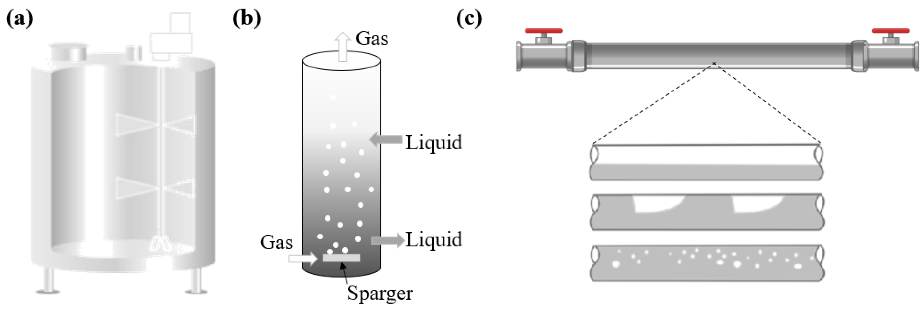
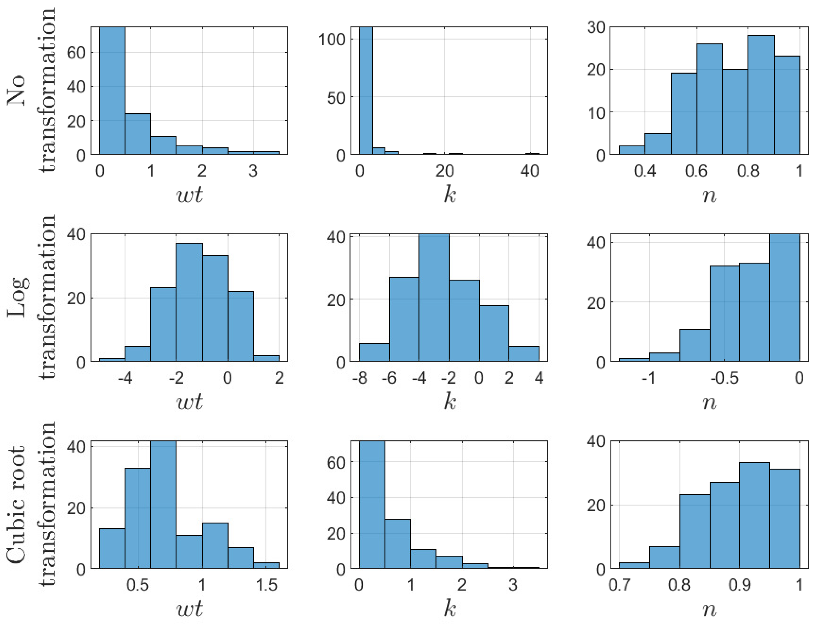
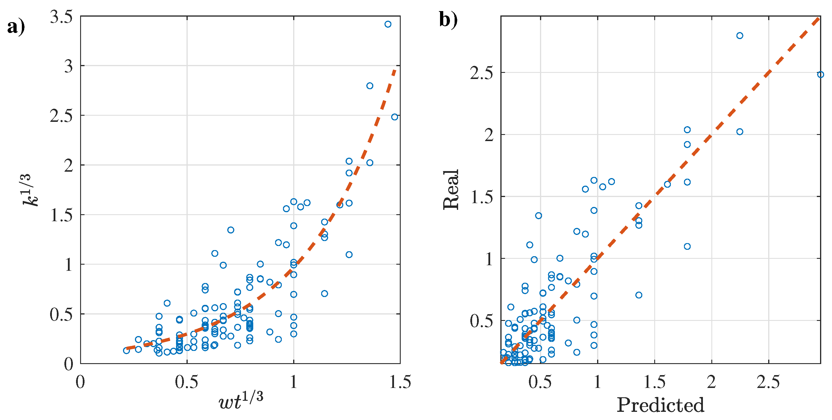
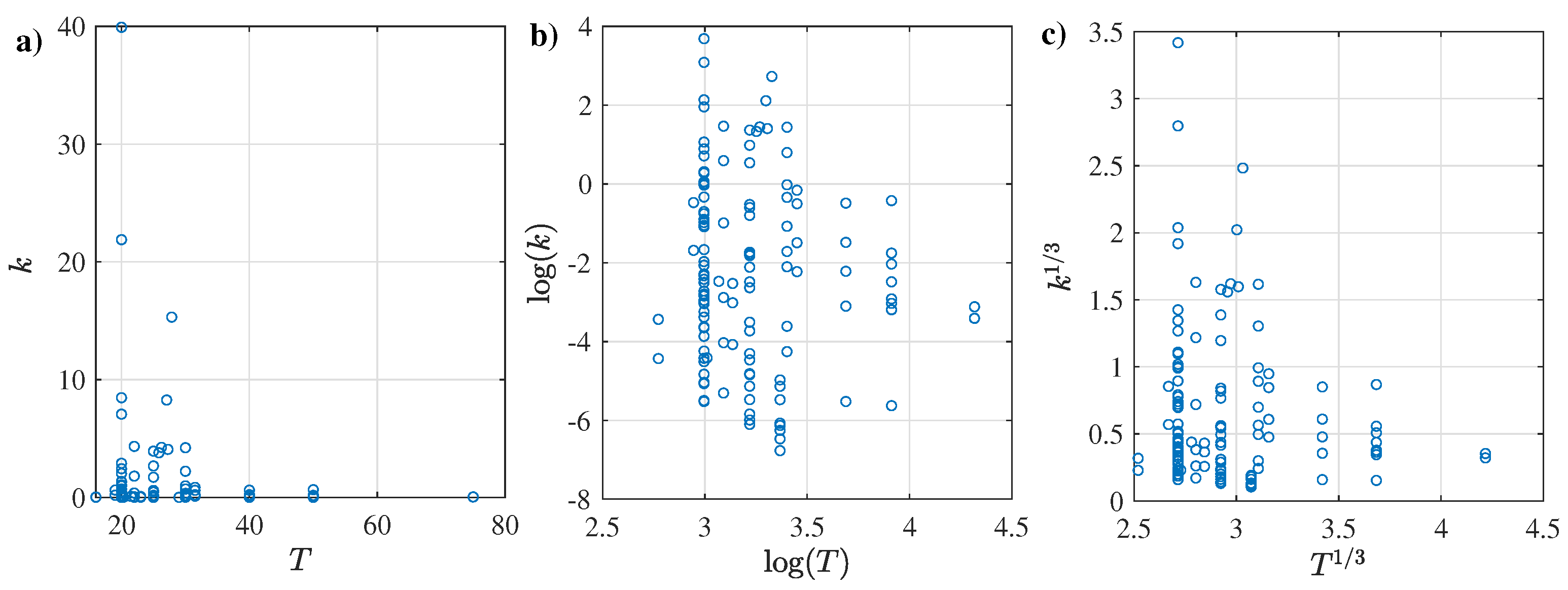


| Author | Main Subject | Main Contribution |
|---|---|---|
| Abukhalifeh et al. [32] | Effect of non-Newtonian flow behavior on the turbulent bed contractor’s hydrodynamic characteristics on a fluidized bed. | High apparent viscosity solutions result in a more densely fluidized bed; the liquid hold-up increases with the high viscosity for different liquid flow rates. |
| Lali et al. [33] | Experimental particle velocities (glass and stainless steel) in viscous non-Newtonian liquids on fluidized beds. | Modified Reynolds number (apparent viscosity) is sufficient to account for increased shear at high Reynolds numbers. |
| Miura and Kawase [34,35]; Miura et al. [27] | Non-Newtonian liquid–solid two-phase in fluidized beds. | Bed voidage augmented with an increase in the liquid velocity. At a given liquid velocity, the magnitude decreases as particle size grows and is more significant as viscosity or viscous non-Newtonian flow behaviors increased. |
| Aydin and Larachi [36] | Effects of temperature and pressure on the hydrodynamics of trickle-bed reactors with Newtonian and non-Newtonian liquids (flow regime transition, pulse velocity, two-phase pressure drop, liquid hold-up, and liquid axial dispersion coefficient). | The trickle-to-pulse flow regime transition boundary shifts to higher fluid velocities with increased temperatures, and pulse velocity increases with temperature. |
| Iliuta et al. [37]; Iliuta and Thyrion [38]; Aydin and Larachi [36]; Iliuta et al. [28] | Hydrodynamics of two-phase down- and up-flow through fixed beds with porous particles (flow regimes, two-phase pressure drops, and liquid hold-ups). | The presence of non-Newtonian liquids strongly influences them. With highly viscous non-Newtonian liquids, the two-phase down-flow hydrodynamic characteristics are close to those of two-phase up-flow. Axial dispersion is an actual cause of possible hydrodynamic effects that can impact reactor performance. |
| Shimizu et al. [29] | Drop size distributions in a stirred tank with a non-Newtonian liquid (CMC and XG) with dispersion process without coalescence. | The non-Newtonian characteristics of the continuous phase caused an increase in the drop size at low impeller speeds. |
| Garcia-Ochoa and Gomez [30] | Oxygen transfer rate in Newtonian and non-Newtonian fluids in a stirred tank. | The volumetric mass transfer coefficient was determined to change many variables (i.e., superficial gas velocity, stirrer speed, and the liquid’s rheologic properties). |
| Sindall et al. [39] | Positron emission particle tracking (PEPT) to visualize the flow patterns on an anaerobic digester fitted with mechanical or gas mixing systems. | Sewage sludge and a transparent synthetic sludge (CMC) calculated the digester’s velocity profiles. PEPT was used to accurately validate CFD models, which could be used to optimize flow patterns for biogas production. |
| Author | Main Subject | Main Contribution |
|---|---|---|
| Das and Biswas [49]; Biswas and Das [48] | Two-phase pressure drop in vertical tubes and helical coils using gas–non-Newtonian liquid. | Analysis of the effects of the gas flow rate, liquid flow rate, concentrations of CMC, and coil diameter on the pressure drop. |
| Dziubinski [50,51]; Dziubinski et al. [52]; Dziubinski and Marcinkowski [53]; Fidos et al. [54] | Pressure drop and void fraction for two-phase flow in vertical pipes using non-Newtonian liquids. | The generalized Reynolds number resulting from the power-law (non-Newtonian) liquid model cannot be used to determine the Taylor bubble rising velocity. |
| Jinming and Jingxuan [55]; Xu et al. [56]; Xu and Wu [57]; Xu et al. [58] | Upward and downward two-phase flow in horizontal, inclined, and vertical pipes using non-Newtonian liquids. | Measurement of void fraction and pressure drop to develop a void fraction and pressure gradient model validated against a large set of available experimental data over a wide range of operating conditions, fluid characteristics, and pipe diameters. |
| Yang et al., [59] and Zhang et al. [60] | Two-phase flow of nitrogen/non-Newtonian fluid (CMC and XG) in non-circular and circular microchannels, respectively. | Flow pattern maps based on observation. |
| Fan et al. [61] | Flow field around two parallel bubbles rising from two uniform orifices submerged in non-Newtonian liquid using Particle Imaging Velocimetry (PIV). | The fluid velocity in front of and behind two bubbles increases with gas flow rate due to the CMC solution’s shear-thinning effect. However, the speed decreases with increasing solution concentration due to the rising drag force acting on the bubbles. |
| Sousa et al. [62,63] | Flow around a single Taylor bubble rising in non-Newtonian solutions using PIV and shadowgraphy (the bubble interface’s correct position and different shapes of bubbles) | Flow around the nose of the bubbles was similar to that around all the bubbles. Velocity profiles in the liquid film around the bubble and the tail (wake region) formed different structures. This result was attributed to the increase in viscosity, and the wake flow pattern varied from turbulent to laminar. In addition, a negative wake was observed for solutions with higher polymer concentrations. |
| Araujo et al. [64] | A CFD study about the rise of individual Taylor bubbles through CMC. | Detailed predictions of viscosity and shear rate distributions that are unattainable with experimental techniques. Application of CFD tools to describe this system was successfully validated against experimental data obtained from photography and PIV/PST measurements of individual Taylor bubbles. |
| Author | Description | |
|---|---|---|
| Wachi et al. [70] | Gas hold-up and liquid circulation rates in a bubble column with Newtonian and non-Newtonian liquids. | Fluid properties (i.e., viscosity and surface activity) affected gas hold-up between riser and downcomer and consequent liquid circulation. High viscosity and low surface tension of Newtonian liquids (glycerol and ethanol, respectively) reduced the circulation rate compared to water, whereas non-Newtonian fluids (CMC) increased liquid velocities. |
| Deng et al. [71] | Gas hold-up, bubble behavior (size and shape), interfacial area, and gas–liquid mass transfer in a bubble column. | Increasing the bubble velocity or CMC concentration led to a broader bubble size distribution. The mass transfer coefficient increased with increasing bubble velocity and decreasing CMC concentration. |
| Fransolet et al. [72] | Experimental analysis of fluid rheology’s influence on the gas flow pattern in a bubble column reactor. Bubble size distributions were measured using parietal pressure probes; the gas hold-up and air distribution were determined by 2D electrical resistance tomography (ERT) images of the gas distribution within the bubble column. | The gas flow pattern within the column was different for Newtonian and non-Newtonian fluids. Gas hold-up values decreased with increasing liquid viscosity, reaching a plateau. A homogeneous flow regime at low gas velocities tended to disappear when viscosity increased. |
| Babaei et al. [73] | Electrical resistance tomography (ERT) measurements as a non-intrusive approach to examining the influence of MLSS concentration and aeration intensity on gas hold-up within the bioreactor. | Gas hold-up was a determinant factor regarding the efficiency of AS processes. An increase in MLSS concentration led to an initial increase followed by decreasing variation in overall gas hold-up. |
| Bajon Fernandez et al. [74] | Gas-to-liquid mass transfer in digested sludge (shear-thinning fluid) and the impact of apparent viscosity on process performance using a pilot-scale absorption bubble column for Newtonian and shear-thinning fluids with different superficial gas velocities. | A reduction of mass transfer efficiency with increasing viscosity was observed. Conditions imitating the rheological variability of anaerobically digested sewage sludge were included with CMC. Rheology should be accounted for in the design of mass transfer systems to avoid reductions in process performance and active volume. |
| Passos et al. [75] | Observation of organic surface-active agents’ effect in bubble column equipped with a porous sparger containing a non-Newtonian liquid (XG). | The diameter of the bubbles decreased as a function of the gas flow rate. |
| Cao et al. [76] | Use of XG as surrogate fluid for digested sludge due to its excellent optical clarity and stability. | The rheological behavior of XG was similar to sludge; it followed the same trend in the rheological curves, with similar curvatures. |
| Bobade et al. [77,78,79] | Gas injection influence on the rheological properties of XG was used to model sludge. | The XG flow curve showed negligible change in apparent viscosity in the flow region as the gas injection flow rate increased. However, a creep test strengthened the molecular structure in the linear viscoelastic region. This means that XG is unsuitable as a model fluid for the sludge under gas injection below the yield stress point. |
| Dong et al. [80] | Experimental examination of mass transfer performance in CMC. | Liquid phase rheology had a significant effect on gas–liquid mass transfer performance. CMC’s volumetric mass transfer coefficients were much smaller than those of water. |
| Bohm et al. [81] | Bubble swarm behavior in a flat sheet MBR. The channel depth, superficial liquid and gas velocity parameters, and continuous phase viscosity were varied. Along with water, XG was used as a non-Newtonian liquid to investigate the rheology of actual wastewater sludge. | Significant influence on the rheology was found for both measured properties, indicating that the results gained in water are not transferable to entire systems. |
| Concentration Range (wt.%) | k Range (Pa sn) | n Range (–) | Shear Rate Range (s−1) | T (°C) | Geometry | Rheometer | Ref. |
|---|---|---|---|---|---|---|---|
| 0.20–1.00 | 0.0041–0.0266 | 0.90–0.98 | 10–1200 | 20 | NM | AR 2000-TA Instruments | [32] |
| 0.90–3.20 | 3.7900–15.3100 | 0.61–0.79 | 0.1–200 | 25–28 | CC | Bohlin CVO-100 | [89] |
| 0.25 | 0.0330–0.0720 | 0.66–0.71 | 0–1000 | 25–75 | NM | Advanced Rheometric Expansion System (ARES) | [36] |
| 0.20–3.00 | 0.0584–39.9221 | 0.36–0.62 | 0–1000 | 20 | CP | AR 2000-TA Instruments | [90] |
| 0.02–0.08 | 0.0142–0.7112 | 0.60–0.90 | NM | 30 | T | pipeline viscometer | [48] |
| 0.05–0.20 | 0.0040–0.0520 | 0.72–0.91 | NM | NM | NM | NM | [91] |
| 0.50–0.70 | 0.0119–0.0322 | 0.92–0.99 | 0–1000 | 16 | DG | RHEOTEC RC 20 | [92] |
| 0.20–0.40 | 0.0135–0.1211 | 0.67–0.87 | NM | 25 | NM | Haake Rotovisco | [31] |
| 0.2–0.8 | 0.054–1.336 | 0.619–0.805 | 100–500 | 35 | CC | AR1000 | [69] |
| 0.05–0.10 | 0.1080–0.8530 | 0.65–0.80 | NM | 31.5 | T | pipeline viscometer | [49] |
| 0.20–0.45 | 0.0065–0.0973 | 0.73–0.96 | NM | NM | NM | NM | [71] |
| 0.3–0.6 | 0.043–0.3 | 0.7–0.84 | NM | 20 | CC | Brookfield R/S | [80] |
| 0.50–1.10 | 0.1623–3.9265 | 0.50–0.73 | 5–1230 | 25 | NM | NM | [93] |
| 1.00 | 0.3380 | 0.83 | NM | NM | NM | NM | [51] |
| 0.5–1.5 | 0.024–2.313 | 0.309–0.633 | 0.001–1000 | 25 | CC | SR2000 | [40] |
| 0.35–0.80 | 0.0210–0.1270 | 0.90–0.94 | NM | NM | NM | StressTech REOLOGICA Instruments AB | [61] |
| 1.00–5.00 | 0.0500–28.0000 | 0.53–0.95 | 0.1–1000 | 23 | NM | RS100 Haake | [94] |
| 0.10–2.00 | 0.0120–1.3200 | 0.50–0.80 | NM | NM | NM | NM | [68] |
| 0.10–2.00 | 0.0050–0.0560 | 0.85–0.94 | 62–1007 | 22 | CC | Haake model VT 180 | [38] |
| 0.25–0.50 | 0.0331–0.0834 | 0.66–0.81 | 0–1000 | 25–75 | NM | Advanced Rheometric Expansion System (ARES) | [28] |
| 0.25–2.00 | 0.0270–4.2200 | 0.56–0.84 | 0–2000 | 30 | NM | RV-3 HAAKE | [33] |
| 0.15–0.4 | 0.246–0.733 | 0.421–0.481 | NM | 20 | NM | NM | [44] |
| 0.10–0.25 | 0.0022–0.0069 | 0.85–0.95 | NM | 29 | T | pipeline viscometer | [67] |
| 0.05–0.10 | 0.0012–0.0023 | 0.81–0.84 | NM | 29 | T | pipeline viscometer | [65] |
| 0.01–0.20 | 0.0022–0.1690 | 0.63–0.95 | 163–3254 | 25 | CC | model 35 Farm | [35] |
| 0.03–0.50 | 0.0079–0.5940 | 0.56–0.84 | 163–3254 | 25 | CC | model 35 Farm | [27] |
| 0.10–0.60 | 0.0080–1.0050 | 0.52–0.90 | 100–4000 | 20–50 | CP | PHYSICA model MCR30 | [95] |
| 0.2–0.4 | 0.054–0.209 | 0.73–0.805 | NM | NM | CC | Fann Model 35 | [39] |
| 0.01–0.50 | 0.0036–0.6550 | 0.54–0.91 | 1.5–3254 | 50 | CC | model 35 Farm | [29] |
| 0.10–1.00 | 0.0121–4.3326 | 0.43–0.91 | 0–4000 | 29–25 | NM | AR 2000 - TA Instruments | [62] |
| 0.15–0.30 | 0.0110–0.0390 | 0.80–0.93 | 0.45–660 | 20 | NM | NM | [70] |
| 0.50–2.00 | 0.0660–7.0690 | 0.58–0.86 | NM | 20 | T | capillary tube viscometer | [96] |
| 0.10–0.30 | 0.0170–0.0800 | 0.77–0.85 | NM | 23 | NM | Haake RV1 | [97] |
| 0.10–0.30 | 0.0890–0.9720 | 0.62–0.80 | NM | 20 | DG | ThermoHaake RS300 | [56] |
| 0.05–0.35 | 0.0340–2.4340 | 0.54–0.95 | NM | 20 | DG | ThermoHaake RS300 | [58] |
| 0.40 | 0.3720 | 0.73 | NM | 20 | NM | NM | [13] |
| 0.05–0.25 | 0.0025–0.0059 | 0.92–0.93 | NM | 25 | NM | NM | [60] |
| Set | Expression | RSE | p-Value | |||
|---|---|---|---|---|---|---|
| 3.274 | 0.502 | 643.8192 | 649.4436 | 2.11 × 10⁻²⁰ | ||
| 3.068 | 0.529 | 628.8310 | 637.2676 | 9.54 × 10⁻²² | ||
| 1.543 | 0.784 | 458.6816 | 464.3059 | 1.39 × 10−42 | ||
| 1.514 | 0.591 | 455.0516 | 463.4881 | 1.74 × 10⁻²⁵ | ||
| 0.407 | 0.776 | 130.7712 | 136.3956 | 1.23 × 10−41 | ||
| 0.348 | 0.640 | 93.5095 | 101.9461 | 7.49 × 10⁻²⁹ | ||
| 1.995 | 0.733 | 522.9911 | 531.4277 | 9.32 × 10−37 | ||
| 0.270 | 0.743 | 30.8134 | 39.2500 | 9.60 × 10−38 | ||
| 1.951 | 0.708 | 517.3987 | 525.8352 | 2.29 × 10⁻³⁴ | ||
| 0.462 | 0.264 | 163.2936 | 171.7302 | 7.57 × 10⁻¹⁰ | ||
| 0.248 | 0.765 | 10.2068 | 18.6433 | 4.03 × 10−40 |
| Set | Expression | RSE | p-Value | |||
|---|---|---|---|---|---|---|
| 4.5420 | 0.0413 | 724.3454 | 729.9698 | 1.34 × 10⁻² | ||
| 4.4681 | 0.0017 | 721.2953 | 729.7318 | 2.73 × 10⁻¹ | ||
| 2.3573 | 0.4947 | 563.0005 | 568.6249 | 5.09 × 10⁻²⁰ | ||
| 2.3670 | 0.0010 | 565.0005 | 573.4371 | 2.91 × 10⁻¹ | ||
| 0.5938 | 0.5222 | 223.8186 | 229.4430 | 1.63 × 10⁻²¹ | ||
| 0.5784 | 0.0072 | 218.3740 | 226.8106 | 1.73× 10⁻¹ | ||
| 0.3919 | 0.0014 | 122.5989 | 131.0354 | 2.80 × 10⁻¹ | ||
| 0.2242 | 0.0010 | −14.8137 | −6.3772 | 2.91 × 10⁻¹ | ||
| 0.0654 | 0.0057 | −317.7006 | −309.2640 | 1.96 × 10⁻¹ | ||
| 0.4262 | 0.0023 | 143.2357 | 151.6722 | 2.51 × 10⁻¹ | ||
| 0.2201 | 0.0007 | −19.3121 | −10.8755 | 2.99 × 10⁻¹ | ||
| 0.0677 | 0.0065 | −309.2259 | −300.7893 | 1.83 × 10⁻¹ |
| Set | Expression | RSE | p-Value | |||
|---|---|---|---|---|---|---|
| 0.3515 | 0.8325 | 96.8232 | 108.0719 | 4.97 × 10−47 | ||
| 0.2486 | 0.7625 | 10.6013 | 19.0379 | 8.41 × 10−40 |
| Set | Expression | RSE | p-Value | |||
|---|---|---|---|---|---|---|
| 0.1322 | 0.2367 | −144.705 | −136.268 | 6.99 × 10⁻⁹ | ||
| 0.1858 | 0.2885 | −61.058 | −52.621 | 9.04 × 10⁻¹¹ | ||
| 0.0539 | 0.2983 | −365.250 | −356.814 | 3.87 × 10⁻¹¹ | ||
| 0.0667 | 0.2663 | −313.134 | −304.697 | 6.05 × 10⁻¹⁰ | ||
| 0.0291 | 0.2811 | −517.189 | −508.752 | 1.71 × 10⁻¹⁰ | ||
| 0.0675 | 0.2475 | −310.254 | −301.817 | 2.88 × 10⁻⁹ | ||
| 0.1030 | 0.3070 | −206.011 | −197.575 | 1.80 × 10⁻¹¹ | ||
| 0.0297 | 0.2979 | −511.997 | −503.561 | 4.00 × 10⁻¹¹ |
| Ref. | Concentration Range (wt.%) | k Range (Pa sn) | n Range (–) | Shear Rate Range (s−1) | T (°C) | Geometry | Rheometer |
|---|---|---|---|---|---|---|---|
| [41] | 0.3–0.4 | NM | 0.2–0.45 | 0.001–10 | 23 | CC | HR2 Discovery |
| [78] | 0.3–0.6 | 0.6017–1.275 | 0.283–0.3712 | 0.001–100 | 20 | CC | HR3 |
| [81] | 0.2 | 0.066 | 0.54 | NM | NM | NM | NM |
| [92] | 0.10–0.21 | 0.1110–0.3541 | 0.44–0.54 | 0–1000 | 16 | DG | RHEOTEC RC 20 |
| [76] | 0.15 | 0.0075 | 0.9463 | 2.7–300 | 25 | CC | Haake Viscotester 550 |
| [72] | 0.10–0.50 | 0.1000–2.9300 | 0.19–0.52 | NM | 16 | NM | NM |
| [30] | 0.01–0.20 | 0.0049–0.7076 | 0.32–0.84 | NM | 28 | NM | Brookfield LVT -Synchro-electric |
| [98] | 0.01–0.75 | 0.0015–546.7029 | 0.66–0.96 | 0–4000 | 20 | CP | AR 1000N |
| [35] | 0.01–0.20 | 0.0025–0.2050 | 0.49–0.91 | 163–3254 | 25 | CC | model 35 Farm |
| [27] | 0.10 | 0.0675 | 0.63 | 163–3254 | 25 | CC | model 35 Farm |
| [95] | 0.10–0.20 | 0.0790–0.3700 | 0.39–0.55 | 100–4000 | 20–50 | CP | PHYSICA model MCR30 |
| [29] | 0.25–0.50 | 0.3740–2.1000 | 0.27–0.44 | 1.5–3254 | 50 | CC | model 35 Farm |
| [59] | 0.20 | 0.1685 | 0.52 | NM | 20 | NM | NM |
| Set | Expression | RSE | p-Value | |||
|---|---|---|---|---|---|---|
| 2.0101 | 0.6742 | 185.061 | 188.584 | 5.29 × 10⁻¹² | ||
| 1.2882 | 0.8109 | 147.761 | 153.045 | 1.23 × 10⁻¹⁶ | ||
| 1.3796 | 0.4536 | 152.693 | 156.215 | 3.28 × 10⁻⁷ | ||
| 1.1969 | 0.4514 | 141.439 | 146.723 | 4.88 × 10⁻⁷ | ||
| 35.4541 | 0.8298 | 432.849 | 438.133 | 1.41 × 10⁻¹⁷ | ||
| 0.7525 | 0.7351 | 101.531 | 106.814 | 1.30 × 10⁻¹³ | ||
| 0.8470 | 0.4524 | 111.699 | 116.982 | 4.69 × 10⁻⁷ | ||
| 0.7238 | 0.7437 | 98.180 | 103.464 | 6.58 × 10⁻¹⁴ |
| Set | Expression | RSE | p-Value | |||
|---|---|---|---|---|---|---|
| 1.363 | 0.8502 | 153.563 | 160.607 | 3.66 × 10⁻¹⁷ | ||
| 1.243 | 0.8240 | 146.543 | 155.349 | 2.14 × 10⁻¹⁵ | ||
| 0.720 | 0.7383 | 97.714 | 102.998 | 1.01 × 10⁻¹³ | ||
| 0.833 | 0.9136 | 110.281 | 115.565 | 1.23 × 10⁻²³ | ||
| 0.669 | 0.7826 | 91.385 | 96.669 | 2.20 × 10⁻¹⁵ |
| Set | Expression | RSE | p-Value | |||
|---|---|---|---|---|---|---|
| 0.1974 | 0.12404 | −13.5693 | −8.286 | 1.18 × 10⁻² | ||
| 0.3364 | 0.35920 | 32.2762 | 37.560 | 1.30 × 10⁻⁵ | ||
| 0.0900 | 0.31885 | −81.0937 | −75.810 | 4.78 × 10⁻⁵ | ||
| 0.1070 | 0.40168 | −66.1891 | −60.906 | 3.04 × 10⁻⁶ | ||
| 0.0540 | 0.37371 | −124.9583 | −119.675 | 7.99 × 10⁻⁶ | ||
| 0.1023 | 0.19075 | −70.1112 | −64.828 | 2.00 × 10⁻³ | ||
| 0.1814 | 0.31894 | −20.8249 | −15.541 | 4.76 × 10⁻⁵ | ||
| 0.0538 | 0.33476 | −125.3890 | −120.105 | 2.88 × 10⁻⁵ |
| Set | Expression | RSE | p-Value | |||
|---|---|---|---|---|---|---|
| 0.1074 | 0.4229 | −65.927 | −60.644 | 1.42 × 10⁻⁶ | ||
| 0.0538 | 0.3417 | −125.341 | −120.057 | 2.31 × 10⁻⁵ | ||
| 0.1066 | 0.5161 | −66.581 | −61.297 | 3.51 × 10⁻⁸ | ||
| 0.2107 | 0.5571 | −7.956 | −2.672 | 5.54 × 10⁻⁹ | ||
| 0.0545 | 0.5659 | −124.170 | −118.886 | 3.64 × 10⁻⁹ |
| Ref. | Concentration Range (g/L) | k Range (Pa sn) | n Range (–) | Shear Rate Range (s−1) | T (°C) | Geometry | Rheometer |
|---|---|---|---|---|---|---|---|
| [73] | 0.712–15.86 | 0.00528–0.05371 | 0.6887–0.4136 | 7.7–225.4 | 22 | CC | Bohlin rheometer |
| [78] | 2–3.6 | 0.64–6.788 | 0.278–0.35 | 0.001–100 | 20 | CC | HR3 |
| [6] | 8 | 0.0524 | 0.59 | 0–1000 | 25 | CC | Haake Rheostress RS 75 |
| [69] | 2.5–12.1 | 0.042–5.885 | 0.71–0.367 | 3–702 | 35 | NM | NM |
| [7] | 10 | 0.0130 | 0.72 | 10–1000 | 20 | CC | Rotovisco RV 100 Haake |
| [21] | 2.8–10.2 | 0.0037–0.1245 | 0.4385–0.8268 | 0.001–500 | 20 | T | NM |
| [40] | 3.23 | 0.296 | 0.606 | 1–1000 | 25 | CC | SR2000 |
| [11] | 2.9–12.3 | 0.2783–3.0809 | 0.29–0.51 | NM | 15–30 | NM | NDJ-Model |
| [12] | 2.74–31 | 0.1710–5740 | 0.01–0.10 | 0–1000 | 15–25 | NM | NM |
| [14] | 3.7–22.9 | 0.0053–0.0629 | 0.64–0.89 | 3–1300 | 20 | CC | Rheotest 2.1, Haaken Medingen GMBH |
| [18] | 27–57 | 0.4873–13.2119 | 0.20–0.62 | 0–3000 | 20 | CC & DG | AR 550 |
| [16] | 3–30 | 0.0133–0.1132 | 0.58–0.82 | 3–1300 | 20 | CC | Rheotest 2.1, Haaken Medingen GMBH |
| [10] | 2.7–47 | 0.0202–16.2516 | 0.04–0.67 | 0–2200 | 21 | DG | VT 550 Haake |
| [39] | 17.99 | 0.0036 | 0.073 | NM | NM | CC | Fann Model 35 |
| [8] | 3.3–28.6 | 0.2842–1.1940 | 0.18–0.53 | 0–1850 | 25 | NM | NM |
| [13] | 2.74–16.00 | 0.0090–1.2590 | 0.25–0.73 | 25–1000 | 20 | NM | AR 2000 |
| [9] | 6–16 | 0.0059–0.0068 | 0.56–0.91 | NM | NM | NM | NM |
| Set | Expression | RSE | p-Value | |||
|---|---|---|---|---|---|---|
| 2.3341 | 0.615 | 660.302 | 666.255 | 7.05 × 10⁻³² | ||
| 2.1518 | 0.574 | 637.707 | 646.637 | 1.59 × 10⁻²⁸ | ||
| 1.8867 | 0.290 | 599.571 | 608.502 | 1.67 × 10⁻¹² | ||
| 1.7555 | 0.096 | 590.572 | 599.564 | 7.80 × 10⁻⁵ | ||
| 1.5170 | 0.714 | 536.322 | 545.252 | 6.13 × 10−41 | ||
| 0.3398 | 0.515 | 102.437 | 111.367 | 1.86 × 10⁻²⁴ | ||
| 1.4518 | 0.680 | 523.595 | 532.525 | 2.16 × 10−37 | ||
| 0.5100 | 0.288 | 220.181 | 229.111 | 2.17 × 10⁻¹² | ||
| 0.3232 | 0.556 | 87.933 | 96.864 | 3.15 × 10⁻²⁷ |
| Set | Expression | RSE | p-Value | |||
|---|---|---|---|---|---|---|
| 2.1505 | 0.6733 | 638.512 | 650.419 | 5.68 × 10⁻³⁵ | ||
| 0.4553 | 0.8168 | 188.300 | 200.207 | 9.11 × 10−53 | ||
| 2.1578 | 0.5720 | 640.469 | 655.353 | 1.73 × 10⁻²⁶ | ||
| 0.4564 | 0.4327 | 189.940 | 204.823 | 6.39 × 10⁻¹⁸ | ||
| 1.4870 | 0.7149 | 530.536 | 539.466 | 5.10 × 10−41 | ||
| 0.2842 | 0.2703 | 50.685 | 59.615 | 1.24 × 10⁻¹¹ | ||
| 1.4088 | 0.7607 | 514.869 | 523.799 | 1.84 × 10−46 | ||
| 0.2914 | 0.6398 | 57.929 | 66.859 | 9.89 × 10⁻³⁴ |
| Set | Expression | RSE | p-Value | |||
|---|---|---|---|---|---|---|
| 0.0787 | 0.1467 | −321.760 | −312.830 | 1.19 × 10⁻⁶ | ||
| 0.2447 | 0.0975 | 7.248 | 16.178 | 7.76 × 10⁻⁵ | ||
| 0.0614 | 0.1956 | −393.840 | −384.910 | 1.53 × 10⁻⁸ | ||
| 0.1047 | 0.2743 | −239.043 | −230.113 | 8.35 × 10⁻¹² | ||
| 0.3343 | 0.2712 | 97.712 | 106.642 | 1.13 × 10⁻¹¹ | ||
| 0.0725 | 0.3034 | −345.688 | −336.758 | 4.27 × 10⁻¹³ |
Publisher’s Note: MDPI stays neutral with regard to jurisdictional claims in published maps and institutional affiliations. |
© 2022 by the authors. Licensee MDPI, Basel, Switzerland. This article is an open access article distributed under the terms and conditions of the Creative Commons Attribution (CC BY) license (https://creativecommons.org/licenses/by/4.0/).
Share and Cite
Ratkovich, N.; Amaya-Gómez, R. Membrane BioReactor (MBR) Activated Sludge Surrogate Alternatives Carboxymethyl Cellulose and Xanthan Gum: A Statistical Analysis and Review. Membranes 2022, 12, 909. https://doi.org/10.3390/membranes12100909
Ratkovich N, Amaya-Gómez R. Membrane BioReactor (MBR) Activated Sludge Surrogate Alternatives Carboxymethyl Cellulose and Xanthan Gum: A Statistical Analysis and Review. Membranes. 2022; 12(10):909. https://doi.org/10.3390/membranes12100909
Chicago/Turabian StyleRatkovich, Nicolás, and Rafael Amaya-Gómez. 2022. "Membrane BioReactor (MBR) Activated Sludge Surrogate Alternatives Carboxymethyl Cellulose and Xanthan Gum: A Statistical Analysis and Review" Membranes 12, no. 10: 909. https://doi.org/10.3390/membranes12100909
APA StyleRatkovich, N., & Amaya-Gómez, R. (2022). Membrane BioReactor (MBR) Activated Sludge Surrogate Alternatives Carboxymethyl Cellulose and Xanthan Gum: A Statistical Analysis and Review. Membranes, 12(10), 909. https://doi.org/10.3390/membranes12100909


