Brain Processing of Complex Geometric Forms in a Visual Memory Task Increases P2 Amplitude

 ,
,
Abstract
1. Introduction
1.1. The Study of Visual Working Memory
1.2. Event Related Potentials in the Study of vWM
2. Materials and Methods
2.1. Participants
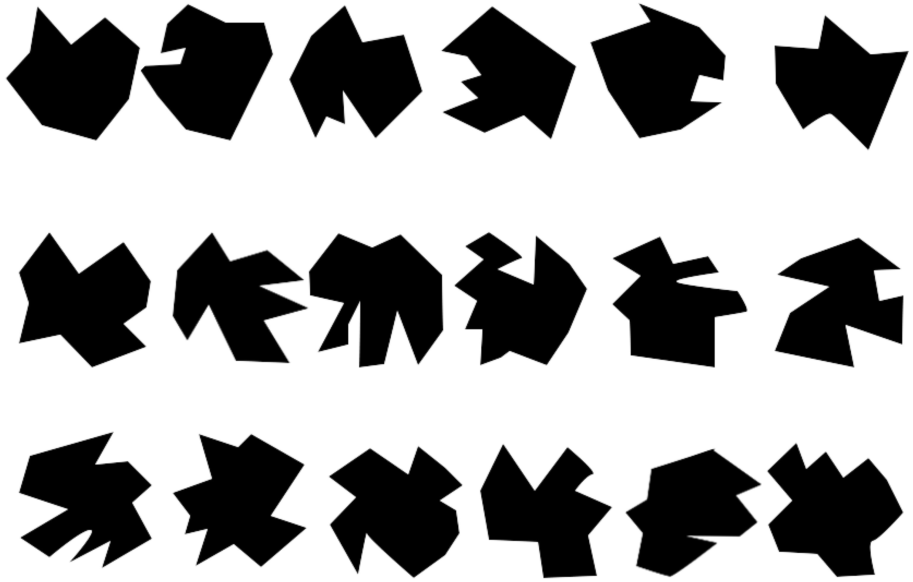
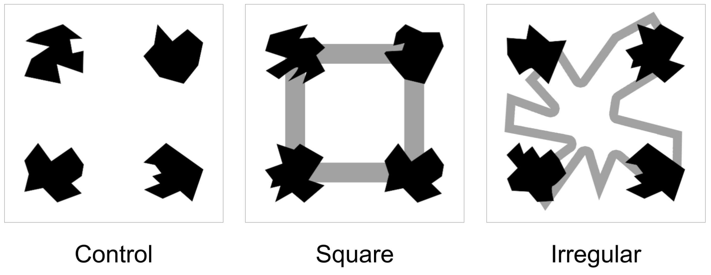
2.2. Materials
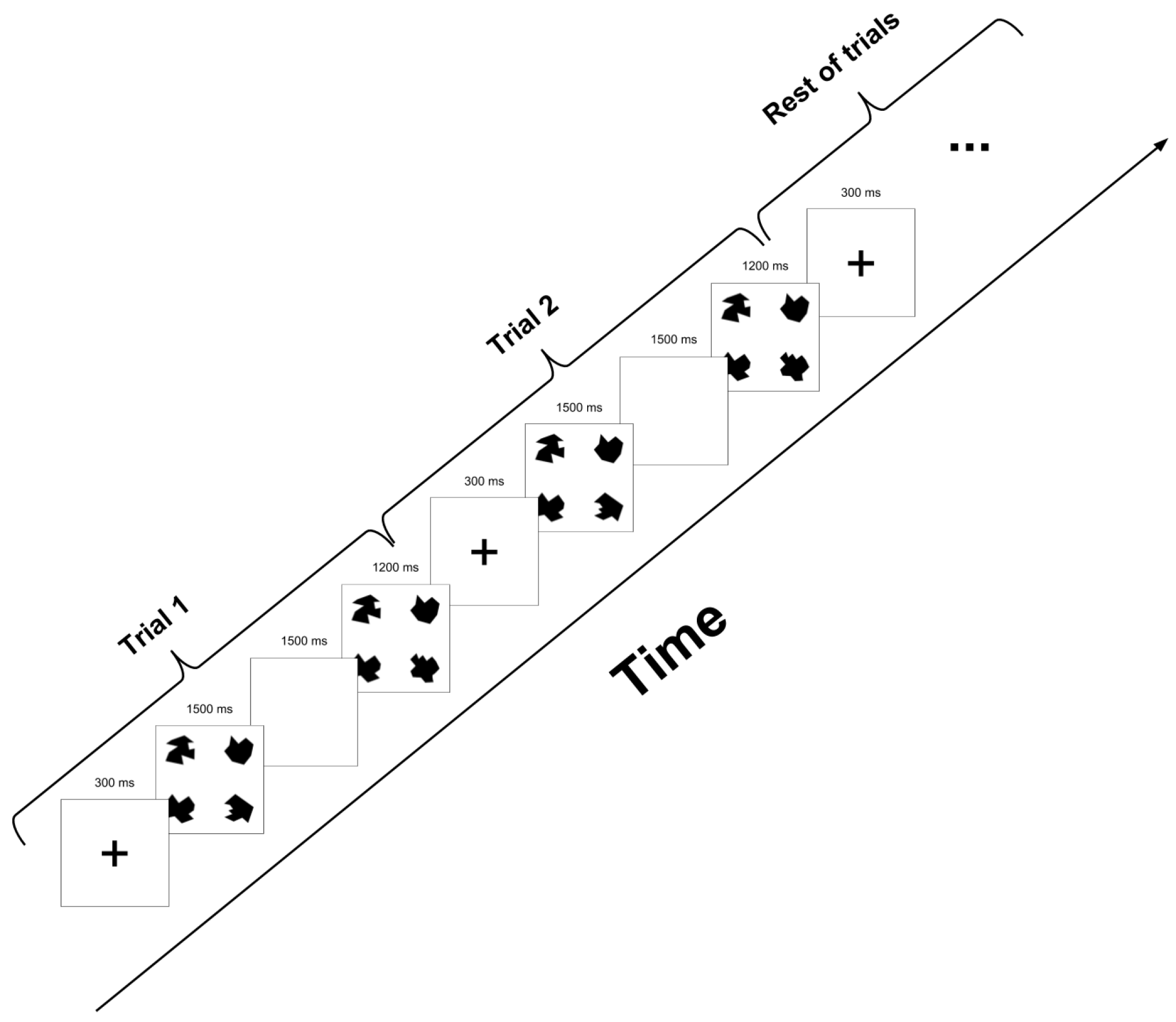
2.3. Experimental Task
2.4. Data Analysis
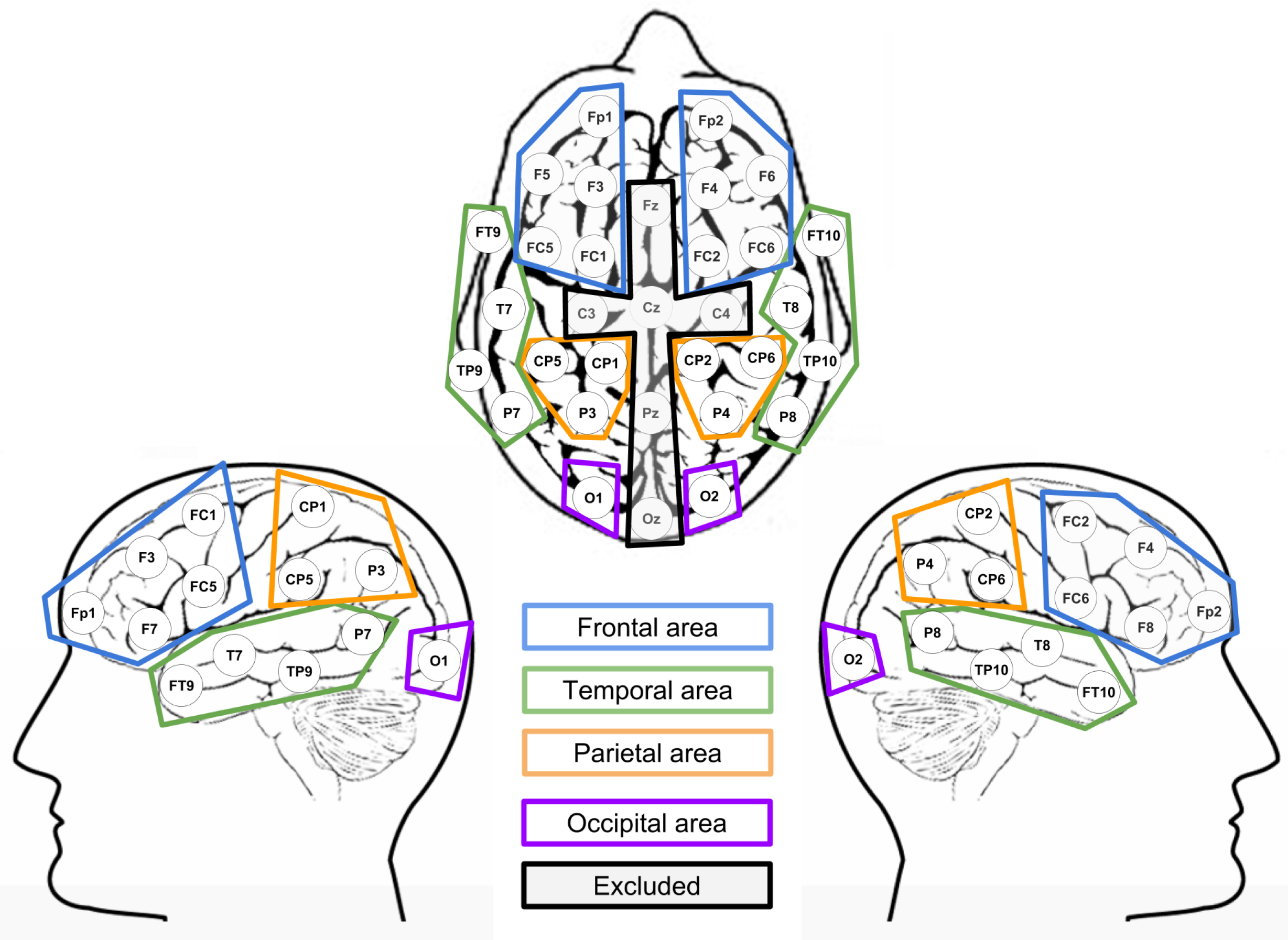
ERP Analysis
3. Results
3.1. Behavioral Results
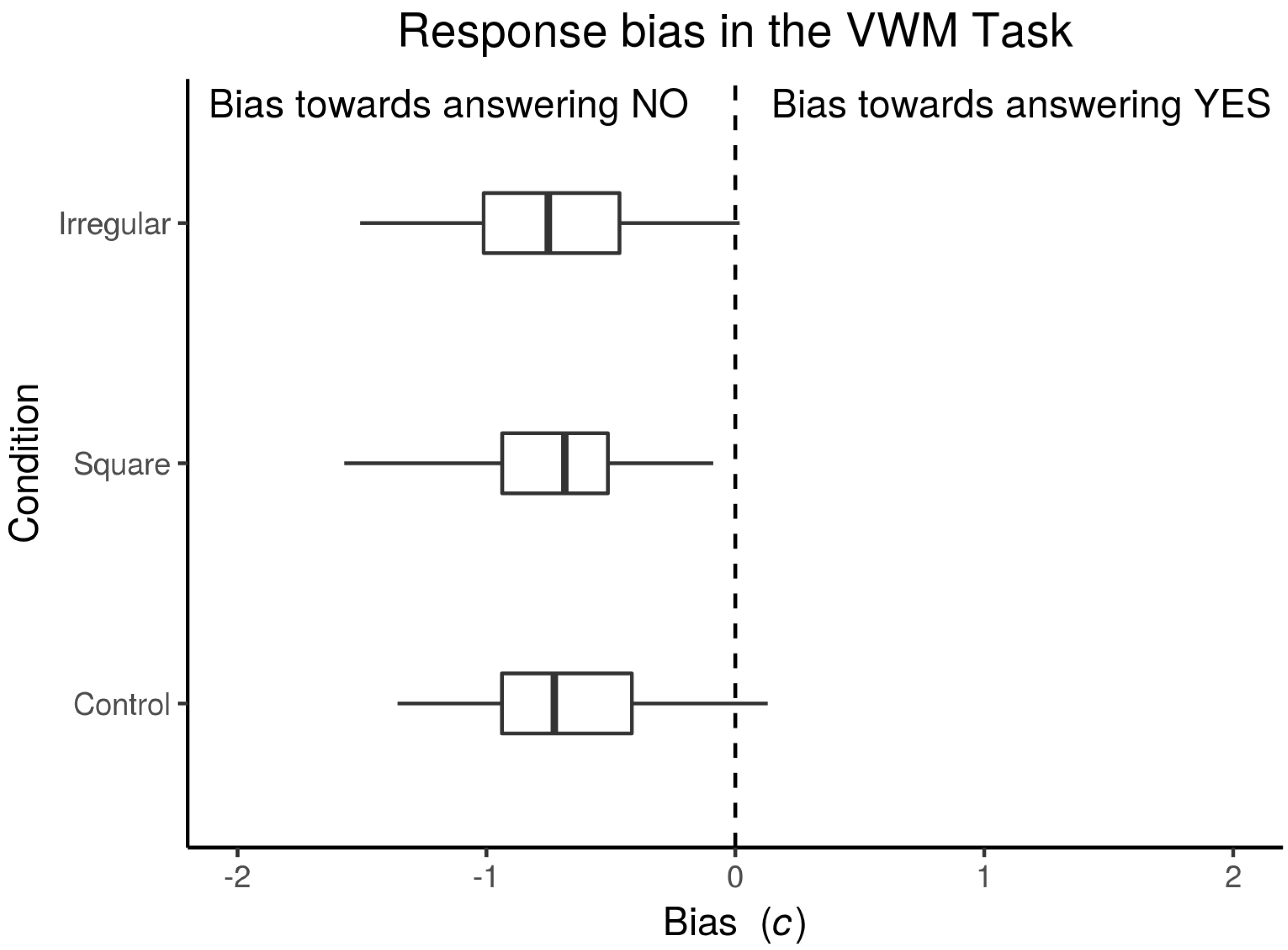
3.1.1. Bias
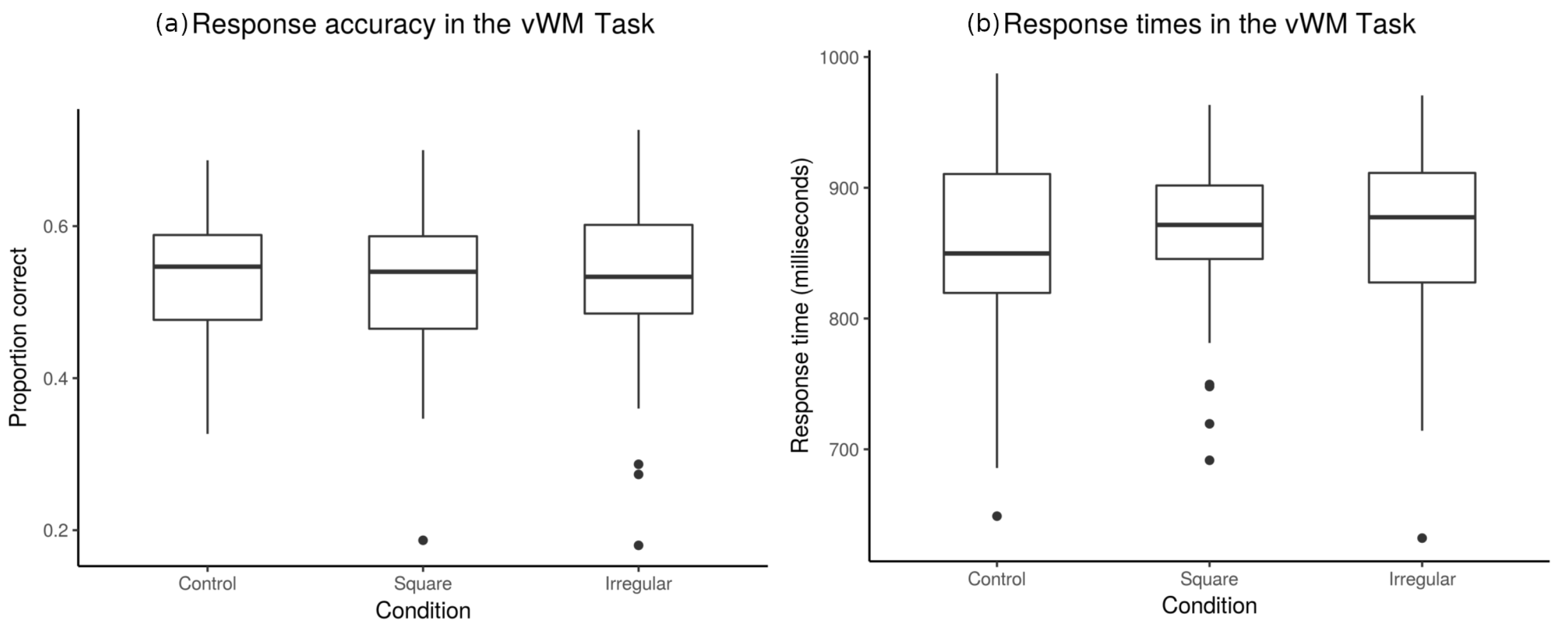
3.1.2. Accuracy and Response Times
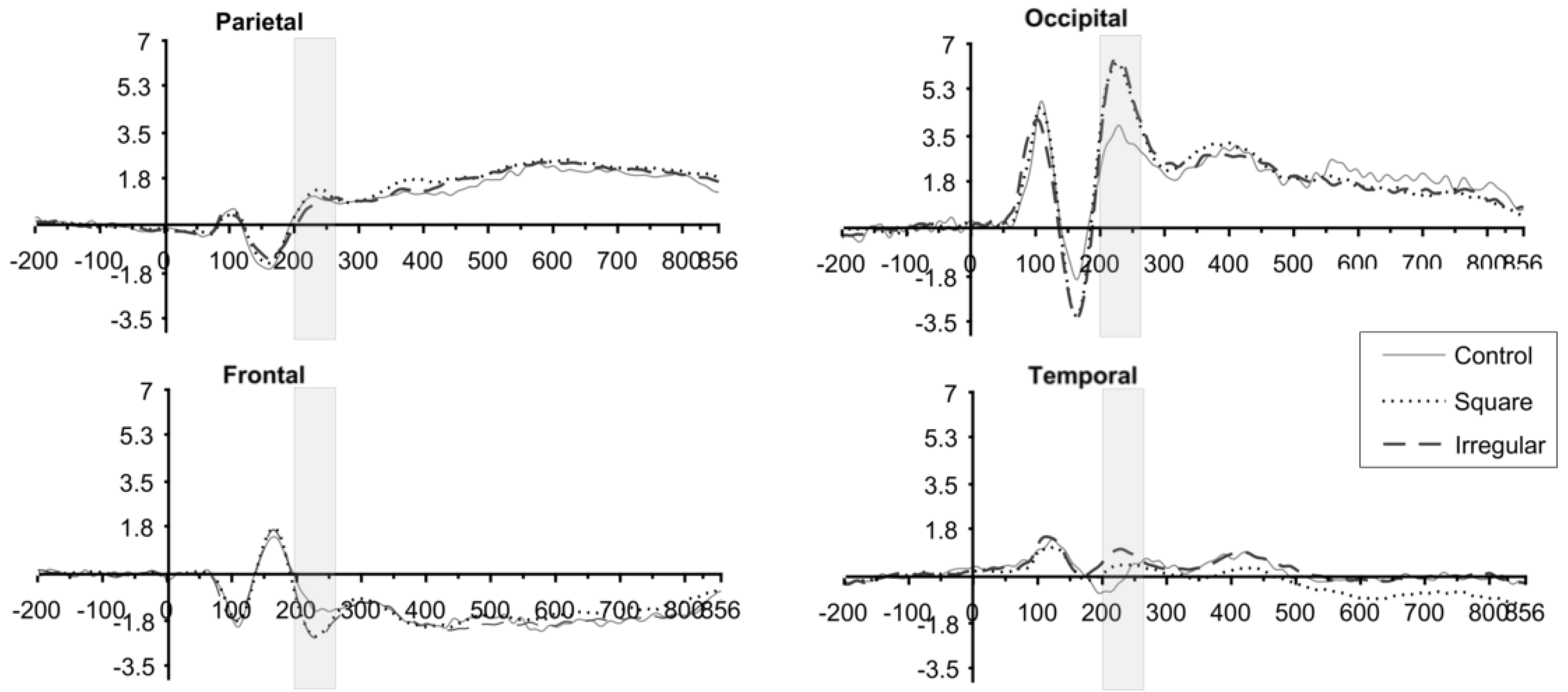
3.2. ERP Results
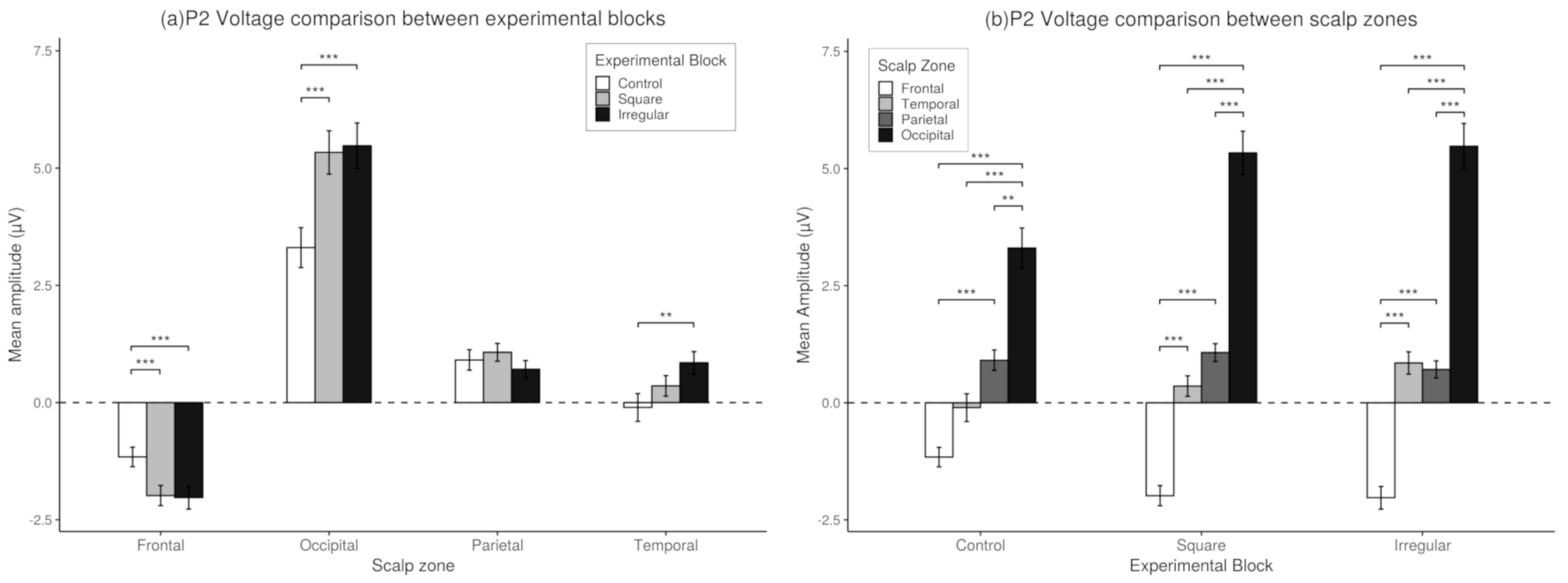
3.3. P2 Analysis
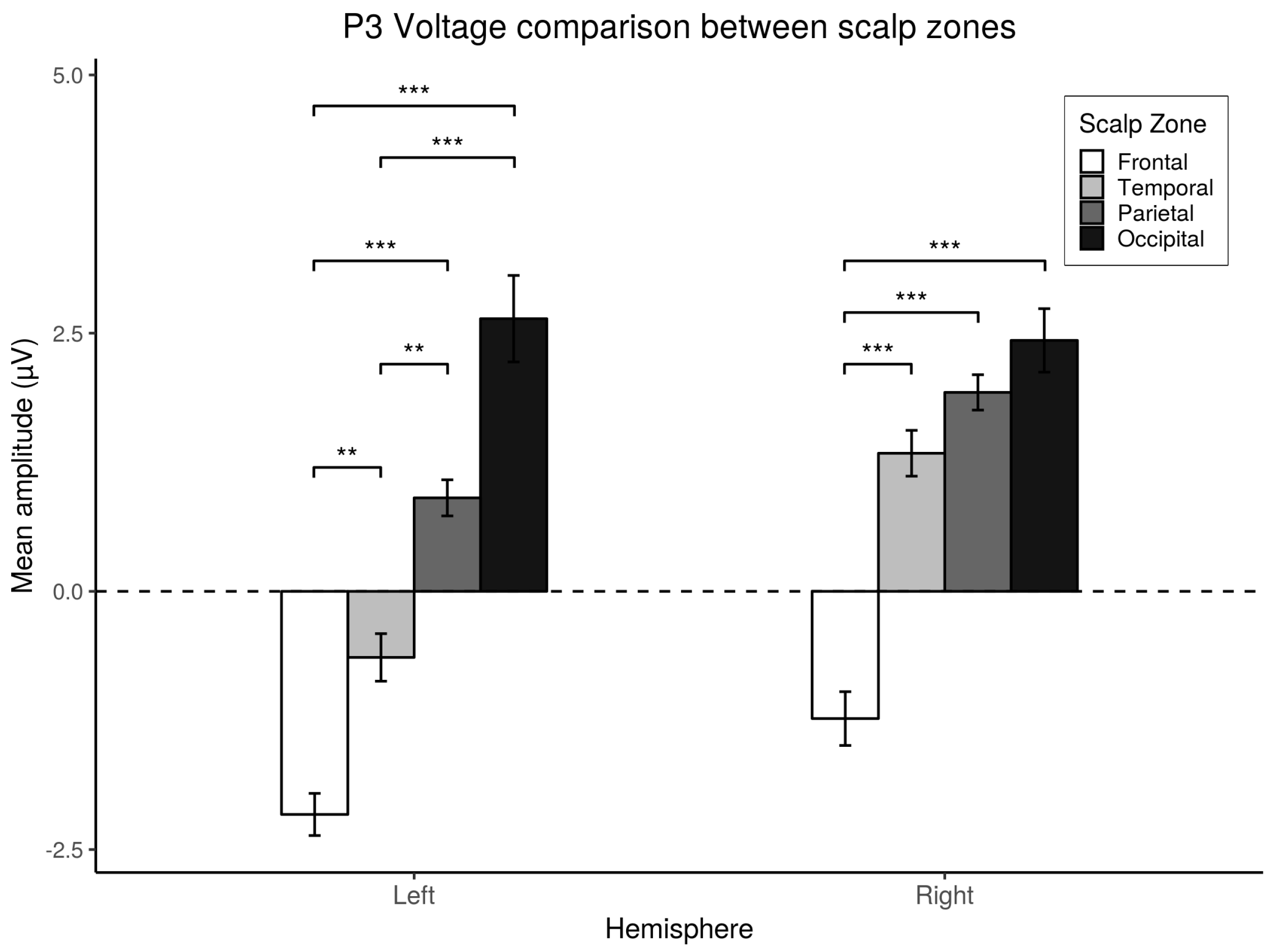
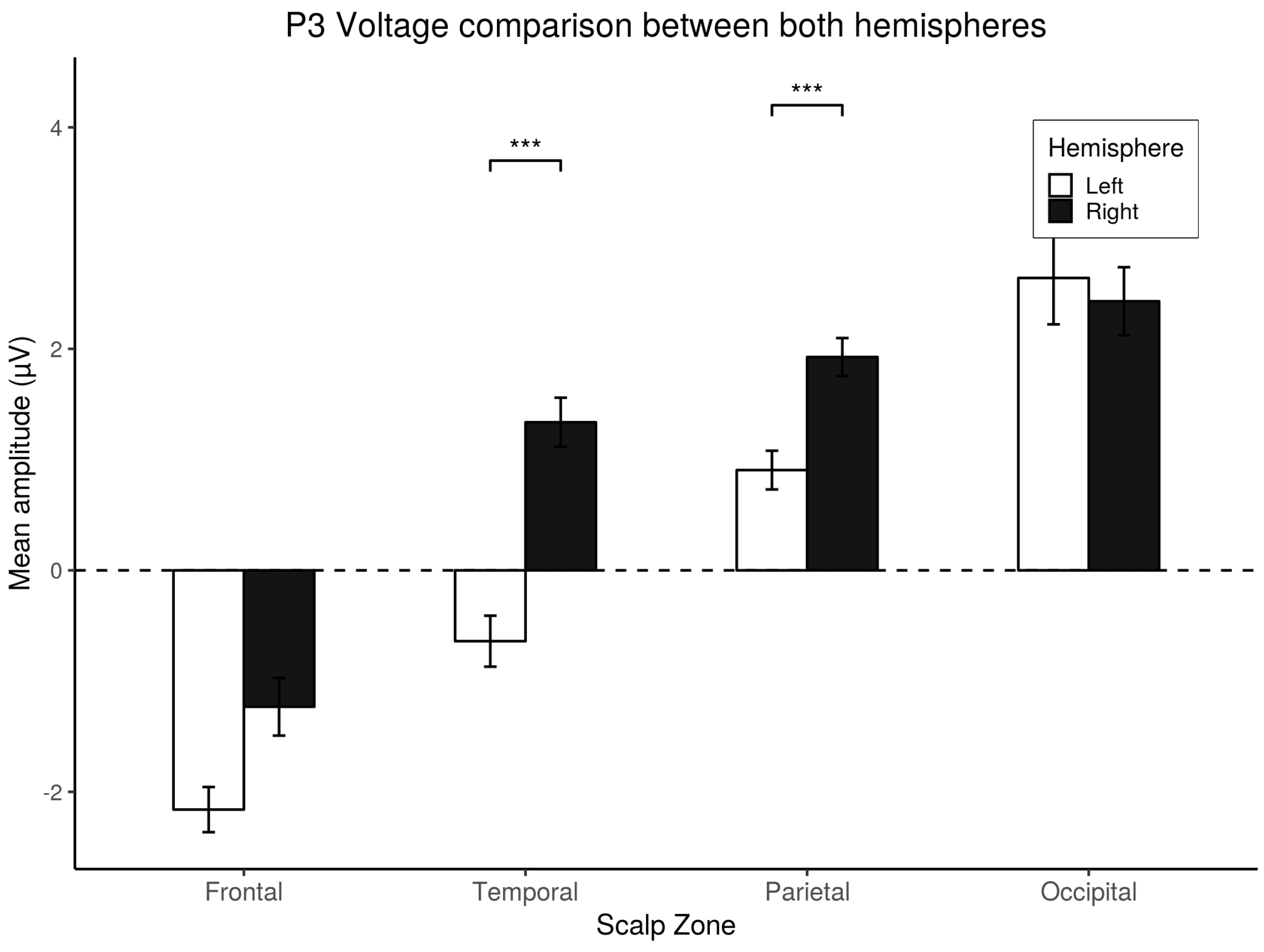
3.4. P3 Analysis
3.5. Behavioral and ERP Interactions
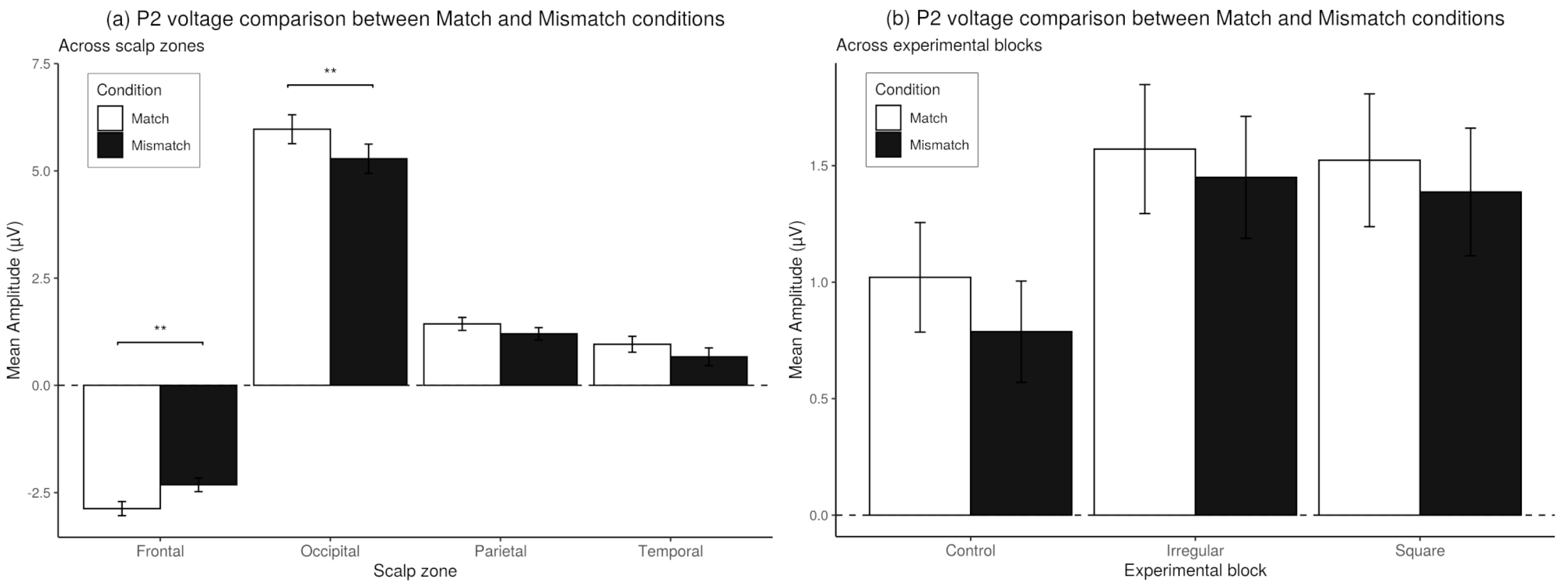
3.6. Match-Mismatch Effects on P2 Amplitude
4. Discussion
Limitations
Author Contributions
Funding
Acknowledgments
Conflicts of Interest
Appendix A
References
- Spencer-Smith, M.; Klingberg, T. Benefits of a working memory training program for inattention in daily life: A systematic review and meta-analysis. PLoS ONE 2015, 10, e0119522. [Google Scholar] [CrossRef]
- Kane, M.J.; Brown, L.H.; McVay, J.C.; Silvia, P.J.; Myin-Germeys, I.; Kwapil, T.R. For whom the mind wanders, and when: An experience-sampling study of working memory and executive control in daily life. Psychol. Sci. 2007, 18, 614–621. [Google Scholar] [CrossRef]
- Johansson, B.; Tornmalm, M. Working memory training for patients with acquired brain injury: Effects in daily life. Scand. J. Occup. Therapy 2012, 19, 176–183. [Google Scholar] [CrossRef] [PubMed]
- Baddeley, A.D.; Hitch, G. Working Memory. In Psychology of Learning and Motivation; Bower, G.H., Ed.; Academic Press: Cambridge, MA, USA, 1974; Volume 8, pp. 47–89. [Google Scholar] [CrossRef]
- Baddeley, A. Working Memory, Thought, and Action, 1st ed.; Oxford University Press: Oxford, UK, 2007; p. 433. [Google Scholar]
- Chun, M.M. Visual working memory as visual attention sustained internally over time. Neuropsychologia 2011, 49, 1407–1409. [Google Scholar] [CrossRef] [PubMed]
- Jarrold, C.; Towse, J.N. Individual differences in working memory. Neuroscience 2006, 139, 39–50. [Google Scholar] [CrossRef] [PubMed]
- Unsworth, N.; Engle, R.W. The nature of individual differences in working memory capacity: Active maintenance in primary memory and controlled search from secondary memory. Psychol. Rev. 2007, 114, 104–132. [Google Scholar] [CrossRef] [PubMed]
- Vogel, E.K.; McCollough, A.W.; Machizawa, M.G. Neural measures reveal individual differences in controlling access to working memory. Nature 2005, 438, 500–503. [Google Scholar] [CrossRef] [PubMed]
- Salthouse, T.A.; Babcock, R.L. Decomposing Adult Age Differences in Working Memory. Dev. Psychol. 1991, 27, 763–776. [Google Scholar] [CrossRef]
- Fukuda, K.; Vogel, E.; Mayr, U.; Awh, E. Quantity, not quality: The relationship between fluid intelligence and working memory capacity. Psychon. Bull. Rev. 2010, 17, 673–679. [Google Scholar] [CrossRef]
- Luck, S.J.; Vogel, E.K. Visual working memory capacity: From psychophysics and neurobiology to individual differences. Trends Cogn. Sci. 2013, 17, 391–400. [Google Scholar] [CrossRef]
- Postle, B.R.; Awh, E.; Serences, J.T.; Sutterer, D.W.; D’Esposito, M. The positional-specificity effect reveals a passive-trace contribution to visual short-term memory. PLoS ONE 2013, 8, e83483. [Google Scholar] [CrossRef] [PubMed]
- Schurgin, M.W.; Flombaum, J.I. Visual working memory is more tolerant than visual long-term memory. J. Exp. Psychol. Hum. Percept. Perform. 2018, 44, 1216. [Google Scholar] [CrossRef] [PubMed]
- Rademaker, R.L.; Park, Y.E.; Sack, A.T.; Tong, F. Evidence of gradual loss of precision for simple features and complex objects in visual working memory. J. Exp. Psychol. Hum. Percept. Perform. 2018, 44, 925. [Google Scholar] [CrossRef] [PubMed]
- Chunharas, C.; Rademaker, R.L.; Sprague, T.C.; Brady, T.F.; Serences, J.T. Separating memoranda in depth increases visual working memory performance. J. Vis. 2019, 19, 4. [Google Scholar] [CrossRef]
- Kessler, Y.; Oberauer, K. Working memory updating latency reflects the cost of switching between maintenance and updating modes of operation. J. Exp. Psychol. Learn. Memory Cogn. 2014, 40, 738. [Google Scholar] [CrossRef]
- McCants, C.W.; Katus, T.; Eimer, M. Task goals modulate the activation of part-based versus object-based representations in visual working memory. Cogn. Neurosci. 2019, 11, 92–100. [Google Scholar] [CrossRef]
- Vandierendonck, A. A working memory system with distributed executive control. Perspect. Psychol. Sci. 2016, 11, 74–100. [Google Scholar] [CrossRef]
- Berch, D.B.; Krikorian, R.; Eileen, M.H. The Corsi Block-Tapping Task: Methodological and Theoretical Considerations. Brain Cogn. 1998, 38, 317–338. [Google Scholar] [CrossRef]
- Brooks, L. The suppression of visualisation by reading. Q. J. Exp. Psychol. 1967, 33A, 1–15. [Google Scholar]
- Logie, R.H. Visuo-spatial working memory: Visual, spatial or central executive? Ment. Images Hum. Cogn. 1991, 80, 105Á. [Google Scholar]
- Luck, S.J.; Vogel, E.K. The capacity of visual working memory for features and conjunctions. Nature 1997, 390, 279–281. [Google Scholar] [CrossRef] [PubMed]
- Kessler, Y.; Rac-Lubashevsky, R.; Lichtstein, C.; Markus, H.; Simchon, A.; Moscovitch, M. Updating visual working memory in the change detection paradigm. J. Vis. 2015, 15, 18. [Google Scholar] [CrossRef] [PubMed]
- Herrmann, C.S.; Knight, R.T. Mechanisms of human attention: Event-related potentials and oscillations. Neurosci. Biobehav. Rev. 2001, 25, 465–476. [Google Scholar] [CrossRef]
- Vogel, E.K.; Luck, S.J. The visual N1 component as an index of a discrimination process. Psychophysiology 2000, 37, 190–203. [Google Scholar] [CrossRef]
- Taylor, M.J. Non-spatial attentional effects on P1. Clin. Neurophysiol. 2002, 113, 1903–1908. [Google Scholar] [CrossRef]
- Luck, S.J.; Heinze, H.J.; Mangun, G.R.; Hillyard, S.A. Visual event-related potentials index focused attention within bilateral stimulus arrays. II. Functional dissociation of P1 and N1 components. Electroencephalogr. Clin. Neurophysiol. 1990, 75, 528–542. [Google Scholar] [CrossRef]
- Friedman, D.; Cycowicz, Y.M.; Gaeta, H. The novelty P3: An event-related brain potential (ERP) sign of the brain’s evaluation of novelty. Neurosci. Biobehav. Rev. 2001, 25, 355–373. [Google Scholar] [CrossRef]
- Goldstein, A.; Spencer, K.M.; Donchin, E. The influence of stimulus deviance and novelty on the P300 and Novelty P3. Psychophysiology 2002, 39, 781–790. [Google Scholar] [CrossRef]
- Polich, J.; Kok, A. Cognitive and biological determinants of P300: An integrative review. Biol. Psychol. 1995, 41, 103–146. [Google Scholar] [CrossRef]
- Luck, S.J.; Hillyard, S.A. Electrophysiological correlates of feature analysis during visual search. Psychophysiology 1994, 31, 291–308. [Google Scholar] [CrossRef]
- Freunberger, R.; Klimesch, W.; Doppelmayr, M.; Höller, Y. Visual P2 component is related to theta phase-locking. Neurosci. Lett. 2007, 426, 181–186. [Google Scholar] [CrossRef] [PubMed]
- Finnigan, S.; O’Connell, R.G.; Cummins, T.D.R.; Broughton, M.; Robertson, I.H. ERP measures indicate both attention and working memory encoding decrements in aging. Psychophysiology 2011, 48, 601–611. [Google Scholar] [CrossRef]
- Kotsoni, E.; Csibra, G.; Mareschal, D.; Johnson, M.H. Electrophysiological correlates of common-onset visual masking. Neuropsychologia 2007, 45, 2285–2293. [Google Scholar] [CrossRef] [PubMed]
- Vogel, E.K.; Machizawa, M.G. Neural activity predicts individual differences in visual working memory capacity. Nature 2004, 428, 748–751. [Google Scholar] [CrossRef] [PubMed]
- Nasr, S.; Moeeny, A.; Esteky, H. Neural correlate of filtering of irrelevant information from visual working memory. PLoS ONE 2008, 3, e3282. [Google Scholar] [CrossRef]
- Gao, Z.; Li, J.; Yin, J.; Shen, M. Dissociated Mechanisms of Extracting Perceptual Information into Visual Working Memory. PLoS ONE 2010, 5, 1–15. [Google Scholar] [CrossRef]
- Goodale, M.A.; Milner, A.D. Separate visual pathways for perception and action. Trends Neurosci. 1992, 15, 20–25. [Google Scholar] [CrossRef]
- Portella, C.; Machado, S.; Arias-Carrión, O.; Sack, A.T.; Silva, J.G.; Orsini, M.; Leite, M.A.A.; Silva, A.C.; Nardi, A.E.; Cagy, M.; et al. Relationship between early and late stages of information processing: An event-related potential study. Neurol. Int. 2012, 4, e16. [Google Scholar] [CrossRef]
- Luck, S.J.; Hillyard, S.A. Spatial filtering during visual search: Evidence from human electrophysiology. J. Exp. Psychol. Hum. Percept. Perform. 1994, 20, 1000. [Google Scholar] [CrossRef]
- Talsma, D.; Kok, A. Nonspatial intermodal selective attention is mediated by sensory brain areas: Evidence from event-related potentials. Psychophysiology 2001, 38, 736–751. [Google Scholar] [CrossRef]
- Olivers, C.N.; Peters, J.; Houtkamp, R.; Roelfsema, P.R. Different states in visual working memory: When it guides attention and when it does not. Trends Cogn. Sci. 2011, 15, 327–334. [Google Scholar] [CrossRef] [PubMed]
- Zhou, L.; Thomas, R.D. Principal component analysis of the memory load effect in a change detection task. Vis. Res. 2015, 110, 1–6. [Google Scholar] [CrossRef] [PubMed]
- Quak, M.; Langford, Z.D.; London, R.E.; Talsma, D. Contralateral delay activity does not reflect behavioral feature load in visual working memory. Biol. Psychol. 2018, 137, 107–115. [Google Scholar] [CrossRef] [PubMed]
- Schneider, W.; Eschman, A.; Zuccolotto, A. E-Prime: User’s Guide; Psychology Software Incorporated: Pittsburgh, PA, USA, 2002. [Google Scholar]
- Jasper, H.H. Report of the committee on methods of clinical examination in electroencephalography. Electroencephalogr. Clin. Neurophysiol. Suppl. 1958, 10, 370–375. [Google Scholar] [CrossRef]
- Delorme, A.; Makeig, S. EEGLAB: An open source toolbox for analysis of single-trial EEG dynamics including independent component analysis. J. Neurosci. Methods 2004, 134, 9–21. [Google Scholar] [CrossRef]
- Lopez-Calderon, J.; Luck, S.J. ERPLAB: An Open-Source Toolbox for the Analysis of Event-Related Potentials. Front. Hum. Neurosci. 2014, 8, 213. [Google Scholar] [CrossRef]
- Cowan, N. The magical number 4 in short term memory. A reconsideration of storage capacity. Behav. Brain Sci. 2001, 24, 87–186. [Google Scholar] [CrossRef]
- Kursawe, M.A.; Zimmer, H.D. Costs of storing colour and complex shape in visual working memory: Insights from pupil size and slow waves. Acta Psychol. 2015, 158, 67–77. [Google Scholar] [CrossRef]
- Oberauer, K.; Eichenberger, S. Visual working memory declines when more features must be remembered for each object. Mem. Cogn. 2013, 41, 1212–1227. [Google Scholar] [CrossRef]
- Luria, R.; Sessa, P.; Gotler, A.; Jolicoeur, P.; Dell’Acqua, R. Visual short-term memory capacity for simple and complex objects. J. Cogn. Neurosci. 2010, 22, 496–512. [Google Scholar] [CrossRef]
- Pelli, D.G.; Levi, D.M.; Chung, S.T. Using visual noise to characterize amblyopic letter identification. J. Vis. 2004, 4, 6. [Google Scholar] [CrossRef] [PubMed]
- Malach, R.; Reppas, J.; Benson, R.; Kwong, K.; Jiang, H.; Kennedy, W.; Ledden, P.; Brady, T.; Rosen, B.; Tootell, R. Object-related activity revealed by functional magnetic resonance imaging in human occipital cortex. Proc. Natl. Acad. Sci. USA 1995, 92, 8135–8139. [Google Scholar] [CrossRef] [PubMed]
- Treviño, M.; la Torre-Valdovinos, D.; Manjarrez, E. Noise improves visual motion discrimination via a stochastic resonance-like phenomenon. Front. Hum. Neurosci. 2016, 10, 572. [Google Scholar] [CrossRef] [PubMed]
- Pineles, S.L.; Lee, P.J.; Velez, F.; Demer, J. Effects of visual noise on binocular summation in patients with strabismus without amblyopia. J. Pediatr. Ophthalmol. Strabismus 2014, 51, 100–104. [Google Scholar] [CrossRef] [PubMed]
- Schupp, H.T.; Stockburger, J.; Schmälzle, R.; Bublatzky, F.; Weike, A.I.; Hamm, A.O. Visual noise effects on emotion perception: Brain potentials and stimulus identification. Neuroreport 2008, 19, 167–171. [Google Scholar] [CrossRef] [PubMed]
- Talsma, D.; Wijers, A.A.; Klaver, P.; Mulder, G. Working memory processes show different degrees of lateralization: Evidence from event-related potentials. Psychophysiology 2001, 38, 425–439. [Google Scholar] [CrossRef]
- Stanislaw, H.; Todorov, N. Calculation of signal detection theory measures. Behav. Res. Methods Instrum. Comput. 1999, 31, 137–149. [Google Scholar] [CrossRef]
- Widmann, A.; Schröger, E.; Maess, B. Digital filter design for electrophysiological data – a practical approach. J. Neurosci. Methods 2015, 250, 34–46. [Google Scholar] [CrossRef]
- Talsma, D.; Woldorff, M.G. 6 Methods for the Estimation and Removal of Artifacts and Overlap. In Event-Related Potentials: A Methods Handbook; Handy, T.C., Ed.; MIT Press: Cambridge, MA, USA, 2005; p. 115. [Google Scholar]
- Luck, S.J. An Introduction to Event-Related Potentials and Their Neural Origins. In An Introduction to the Event-Related Potential Technique; MIT Press: Cambridge, MA, USA, 2005; Chapter 1; pp. 2–50. [Google Scholar]
- Rugg, M.; Milner, A.; Lines, C.; Phalp, R. Modulation of visual event-related potentials by spatial and non-spatial visual selective attention. Neuropsychologia 1987, 25, 85–96. [Google Scholar] [CrossRef]
- Heinze, H.J.; Luck, S.J.; Mangun, G.R.; Hillyard, S.A. Visual event-related potentials index focused attention within bilateral stimulus arrays. I. Evidence for early selection. Electroencephalogr. Clin. Neurophysiol. 1990, 75, 511–527. [Google Scholar] [CrossRef]
- Fuster, J.M. The Prefrontal Cortex, 4th ed.; Academic Press: Cambridge, MA, USA, 2008. [Google Scholar]
- Smith, E.E.; Jonides, J.; Koeppe, R.A. Dissociating Verbal and Spatial Working Memory Using PET. Cereb. Cortex 1996, 6, 11–20. [Google Scholar] [CrossRef] [PubMed]
- Yamaguchi, S.; Yamagata, S.; Kobayashi, S. Cerebral asymmetry of the “top-down” allocation of attention to global and local features. J. Neurosci. 2000, 20, RC72. [Google Scholar] [CrossRef] [PubMed]
- Hillyard, S.A.; Vogel, E.K.; Luck, S.J. Sensory gain control (amplification) as a mechanism of selective attention: Electrophysiological and neuroimaging evidence. Philos. Trans. R. Soc. Lond. Ser. B Biol. Sci. 1998, 353, 1257–1270. [Google Scholar] [CrossRef] [PubMed]
- Balaban, H.; Luria, R. Object representations in visual working memory change according to the task context. Cortex 2016, 81, 1–13. [Google Scholar] [CrossRef] [PubMed]
- Miller, C.W.; Stewart, E.K.; Wu, Y.H.; Bishop, C.; Bentler, R.A.; Tremblay, K. Working Memory and Speech Recognition in Noise Under Ecologically Relevant Listening Conditions: Effects of Visual Cues and Noise Type Among Adults With Hearing Loss. J. Speech Lang. Hear. Res. 2017, 60, 2310–2320. [Google Scholar] [CrossRef] [PubMed]
- Dunn, B.R.; Dunn, D.A.; Languis, M.; Andrews, D. The relation of ERP components to complex memory processing. Brain Cogn. 1998, 36, 355–376. [Google Scholar] [CrossRef]
- Lefebvre, C.D.; Marchand, Y.; Eskes, G.A.; Connolly, J.F. Assessment of working memory abilities using an event-related brain potential (ERP)-compatible digit span backward task. Clin. Neurophysiol. 2005, 116, 1665–1680. [Google Scholar] [CrossRef]
- Linnert, S.; Reid, V.; Westermann, G. ERP correlates of two separate top-down mechanisms in visual categorization. Int. J. Psychophysiol. 2016, 108, 83. [Google Scholar] [CrossRef]
- Henare, D.T.; Buckley, J.; Corballis, P.M. Working memory availability affects neural indices of distractor processing during visual search. bioRxiv 2018, 295378. [Google Scholar] [CrossRef]
- Gaspar, J.M.; Christie, G.J.; Prime, D.J.; Jolicœur, P.; McDonald, J.J. Inability to suppress salient distractors predicts low visual working memory capacity. Proc. Natl. Acad. Sci. USA 2016, 113, 3693–3698. [Google Scholar] [CrossRef]
- Wolfe, J.M.; Butcher, S.J.; Lee, C.; Hyle, M. Changing your mind: On the contributions of top-down and bottom-up guidance in visual search for feature singletons. J. Exp. Psychol. Hum. Percept. Perform. 2003, 29, 483–502. [Google Scholar] [CrossRef] [PubMed]
- Polich, J. Updating P300: An integrative theory of P3a and P3b. Clin. Neurophysiol. 2007, 118, 2128–2148. [Google Scholar] [CrossRef] [PubMed]


| Effect | Ss | Ms | (Factor) | (Error) | F | p | |
|---|---|---|---|---|---|---|---|
| Block | 45.83 | 22.915 | 2 | 70 | 31.19 | <0.001 | 0.004 |
| Zone | 4654 | 1551.2 | 3 | 105 | 47.55 | <0.001 | 0.444 |
| Hemisphere | 14.7 | 14.69 | 1 | 35 | 1.14 | 0.291 | 0.001 |
| Block*Zone | 238.5 | 39.75 | 6 | 210 | 15.51 | <0.001 | 0.022 |
| Block*Hemisphere | 2.57 | 1.285 | 2 | 70 | 0.63 | 0.545 | <0.001 |
| Zone*Hemisphere | 78.07 | 26.023 | 3 | 105 | 9.40 | <0.001 | 0.007 |
| Block*Zone*Hemisphere | 2.16 | 0.360 | 6 | 210 | 1.02 | 0.383 | <0.001 |
| Effect | Ss | Ms | (Factor) | (Error) | F | p | |
|---|---|---|---|---|---|---|---|
| Block | 0.56 | 0.28 | 2 | 70 | 0.36 | 0.694 | <0.001 |
| Zone | 2102 | 700.8 | 3 | 105 | 20.44 | <0.001 | 0.242 |
| Hemisphere | 186.4 | 186.41 | 1 | 35 | 10.92 | 0.002 | 0.021 |
| Block*Zone | 16.4 | 2.73 | 6 | 210 | 0.776 | 0.535 | 0.001 |
| Block*Hemisphere | 1.88 | 0.9418 | 2 | 70 | 0.437 | 0.625 | <0.001 |
| Zone*Hemisphere | 129.8 | 43.28 | 3 | 105 | 8.705 | 0.001 | 0.014 |
| Block*Zone*Hemisphere | 5.99 | 0.99 | 6 | 210 | 1.908 | 0.127 | <0.001 |
© 2020 by the authors. Licensee MDPI, Basel, Switzerland. This article is an open access article distributed under the terms and conditions of the Creative Commons Attribution (CC BY) license (http://creativecommons.org/licenses/by/4.0/).
Share and Cite
Cepeda-Freyre, H.A.; Garcia-Aguilar, G.; Eguibar, J.R.; Cortes, C. Brain Processing of Complex Geometric Forms in a Visual Memory Task Increases P2 Amplitude. Brain Sci. 2020, 10, 114. https://doi.org/10.3390/brainsci10020114
Cepeda-Freyre HA, Garcia-Aguilar G, Eguibar JR, Cortes C. Brain Processing of Complex Geometric Forms in a Visual Memory Task Increases P2 Amplitude. Brain Sciences. 2020; 10(2):114. https://doi.org/10.3390/brainsci10020114
Chicago/Turabian StyleCepeda-Freyre, Héctor A., Gregorio Garcia-Aguilar, Jose R. Eguibar, and Carmen Cortes. 2020. "Brain Processing of Complex Geometric Forms in a Visual Memory Task Increases P2 Amplitude" Brain Sciences 10, no. 2: 114. https://doi.org/10.3390/brainsci10020114
APA StyleCepeda-Freyre, H. A., Garcia-Aguilar, G., Eguibar, J. R., & Cortes, C. (2020). Brain Processing of Complex Geometric Forms in a Visual Memory Task Increases P2 Amplitude. Brain Sciences, 10(2), 114. https://doi.org/10.3390/brainsci10020114