Generalized Boundary Conditions in Surface Electromagnetics: Fundamental Theorems and Surface Characterizations

Abstract

Generalized boundary conditions (GBCs) for electromagnetic surfaces are investigated in this paper, which can be used to analytically characterize field discontinuities across two-dimensional surfaces. First, five representative features are described to categorize various surface problems which require proper GBC-based characterization procedures. Next, the generalized boundary conditions are discussed in details, in association with impedance boundary conditions, generalized sheet transition conditions, and surface scattering coefficients. Then an extraction method for surface susceptibilities, the characteristic parameters of surfaces in GBCs, are proposed and validated. Finally, to illustrate the applications of GBCs, two representative surface problems are demonstrated, namely, isolated-aperture surface analysis and surface-wave mode characterization. For the isolated-aperture surface, a characterization procedure is derived based on GBCs and Babinet’s principle, and the accuracy is validated through comparison with full-wave simulations. For surface wave analysis, a characterization procedure is also developed from GBCs, and the feasibility is verified by numerical examples as well.

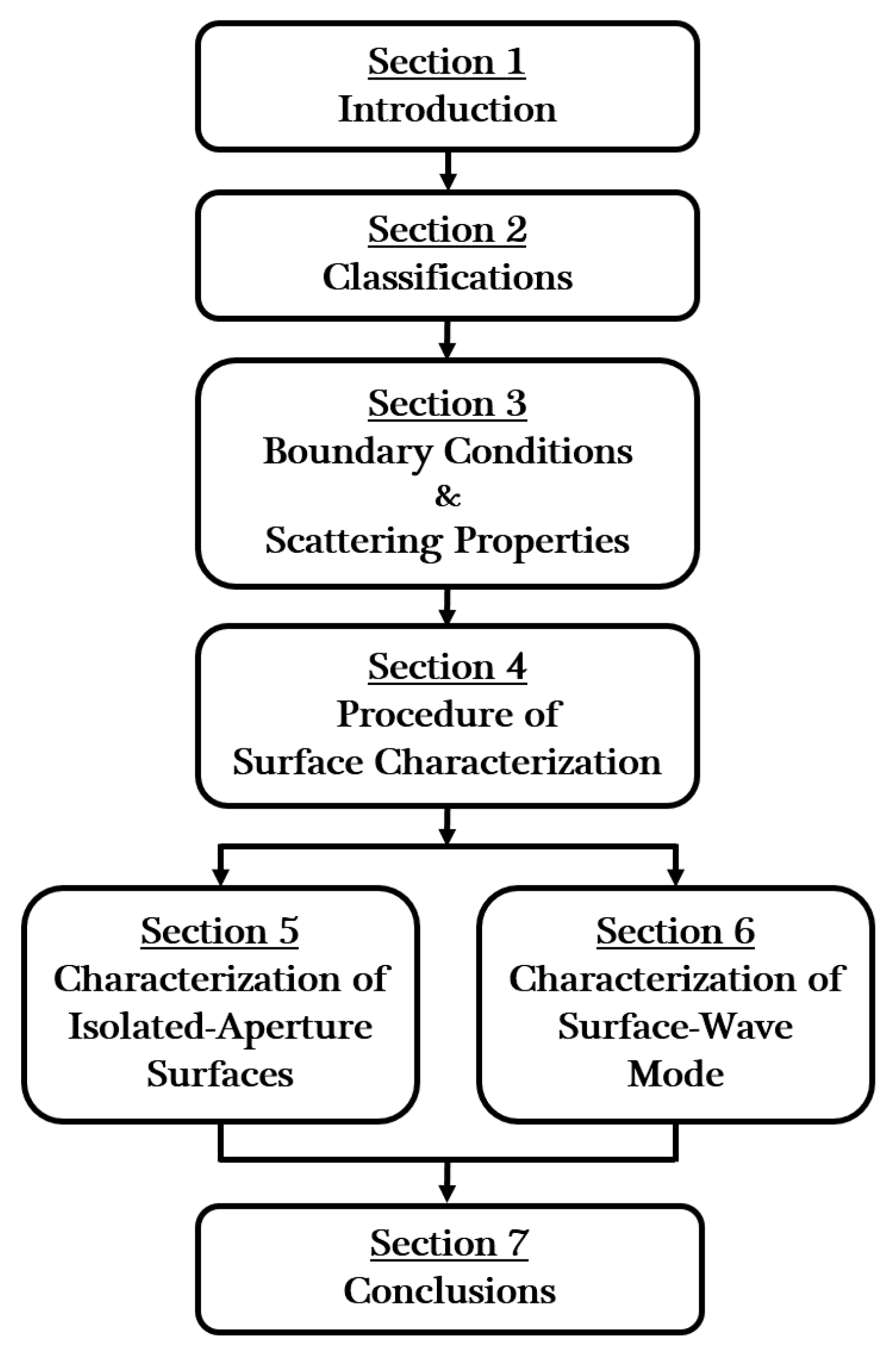
1. Introduction

Surfaces with two-dimensional structures have attracted a great deal of research interests. This is due to many desirable features such as their low profile, light weight and ease of fabrication, as well as their diversified capabilities of manipulating electromagnetic (EM) waves. During the past decades, different kinds of two-dimensional EM surfaces such as frequency selective surfaces (FSS) [1,2,3], electromagnetic band gap (EBG) structures [4,5,6] and metasurfaces (MTS) [7,8,9] have been studied in depth, leading to diversified applications which realize various kinds of functions.

To comprehensively understand EM surfaces, it is necessary to locate surface problems among overall EM studies. In respect to spatial dimensions, EM problems can be categorized according to the electrical size of structures interacting with EM fields. As shown in Figure 1, where dimensions along different directions in Cartesian coordinates are designated as $L_x$, $L_y$ and $L_z$ respectively, all EM problems are classified into four types:

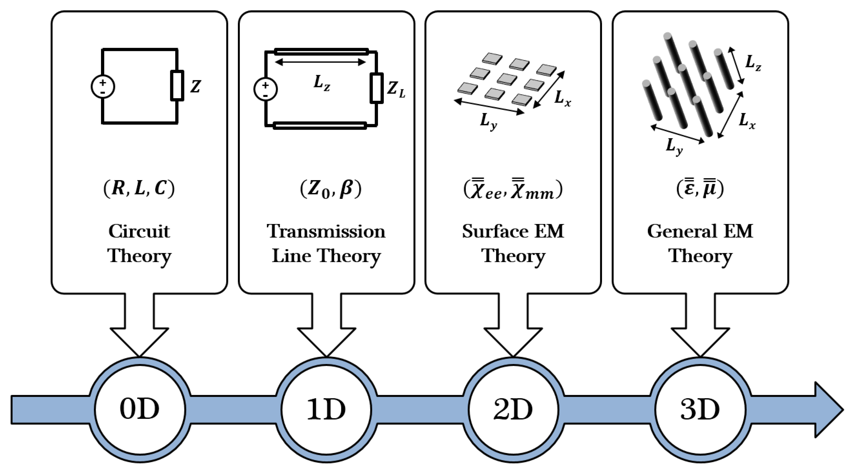
• 3D EM problems. For structures with $L_x$, $L_y$ and $L_z$ all comparable to wavelength $\lambda$, they are usually discussed with three-dimensional electromagnetics, which is analyzed by general EM theory. For 3D problems, permittivity $\epsilon$ and permeability $\mu$ are utilized to characterize properties of homogeneous mediums while their effective counterparts are defined for inhomogeneous ones. The corresponding mathematical tools are derived from Maxwell’s equations.
• 0D EM problems. In contrast, if all dimensions are much smaller than $\lambda$, problems can be addressed with the zero dimension approach through description by lumped parameters. As a result, these problems can be analyzed with circuit theory. For 0D problems, structures can be represented by lumped circuit parameters, such as resistance R, inductance L and capacitance C. Field relations are consistent with Kirchhoff’s laws.
• 1D EM problems. If transverse dimensions $L_x$ and $L_y$ are much smaller than $\lambda$, these one-dimensional problems can be solved with transmission line theory. For 1D problems, the characteristic impedance $Z_0$ and propagation constant $\beta$ are the principal parameters which comply with transmission line equations [10].
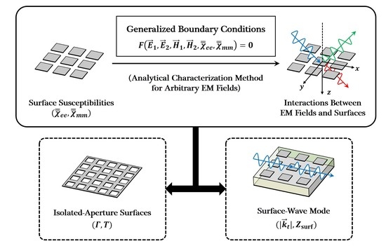
• 2D EM problems. When only the longitudinal dimension $L_z$ becomes much smaller than $\lambda$, characterization of these two-dimensional surfaces can be denominated as theory of surface electromagnetics (SEM). For 2D problems, the most appropriate characterization parameters are effective surface susceptibilities ${\overline{\overline{\chi }}}_{ee}$ and ${\overline{\overline{\chi }}}_{mm}$ [11], while related mathematical models are named as generalized boundary conditions (GBCs).

This begs the question of how GBCs differ from conventional boundary conditions. In surface electromagnetics, field discontinuities across engineered surfaces are deliberately designed in order to manipulate or transform EM waves [12,13,14], and boundary conditions are used to describe these field discontinuities. In conventional boundary conditions, field discontinuities are attributed to current sources distributed along surfaces, as shown in Figure 2. Meanwhile, the current sources are dependent not only on the surface characteristics but also on the applied fields. Thus, the EM fields and the current sources are coupled together. As a result, it is not straightforward and sometimes even complicated to solve field discontinuities with conventional boundary conditions.

To overcome this difficulty, an alternative approach to determine the field discontinuities directly from the surface characteristics exists: generalized boundary conditions (GBCs). It is worthwhile to point out that the surface characteristics here are eigen-parameters of surfaces dependent on surface geometry and material, but independent of applied fields. Once their values have been determined, the field discontinuities across surfaces are expected to be analytically computed for applied fields with arbitrary propagation directions and polarizations.

A significant amount of research focuses on generalizing the EM boundary conditions, such as impedance boundary conditions (IBCs) [15,16,17], generalized sheet transition conditions (GSTCs) [7,11,18], and general linear and local conditions [19,20]. These approaches have been applied to specific kinds of surfaces with satisfactory results. Due to the vast diversity of various engineered EM surfaces, GBCs still require further exploration in order to characterize general EM surfaces analytically.

The remainder of this paper is organized as follows: Section 2 describes the classification of two-dimensional surface problems according to different features while Section 3 reviews various boundary conditions, scattering properties of surfaces, and the relationship between the two. Section 4 demonstrates how to extract characteristic parameters from limited sets of simulations and utilize them to compute scattering coefficients for arbitrary situations. In Section 5 and Section 6, analytical solutions to the issues of isolated-aperture surfaces and surface-wave mode are proposed respectively. Finally, Section 7 presents the conclusions. To help visualization, a flow chart depicting the organization of this paper is shown in Figure 3.

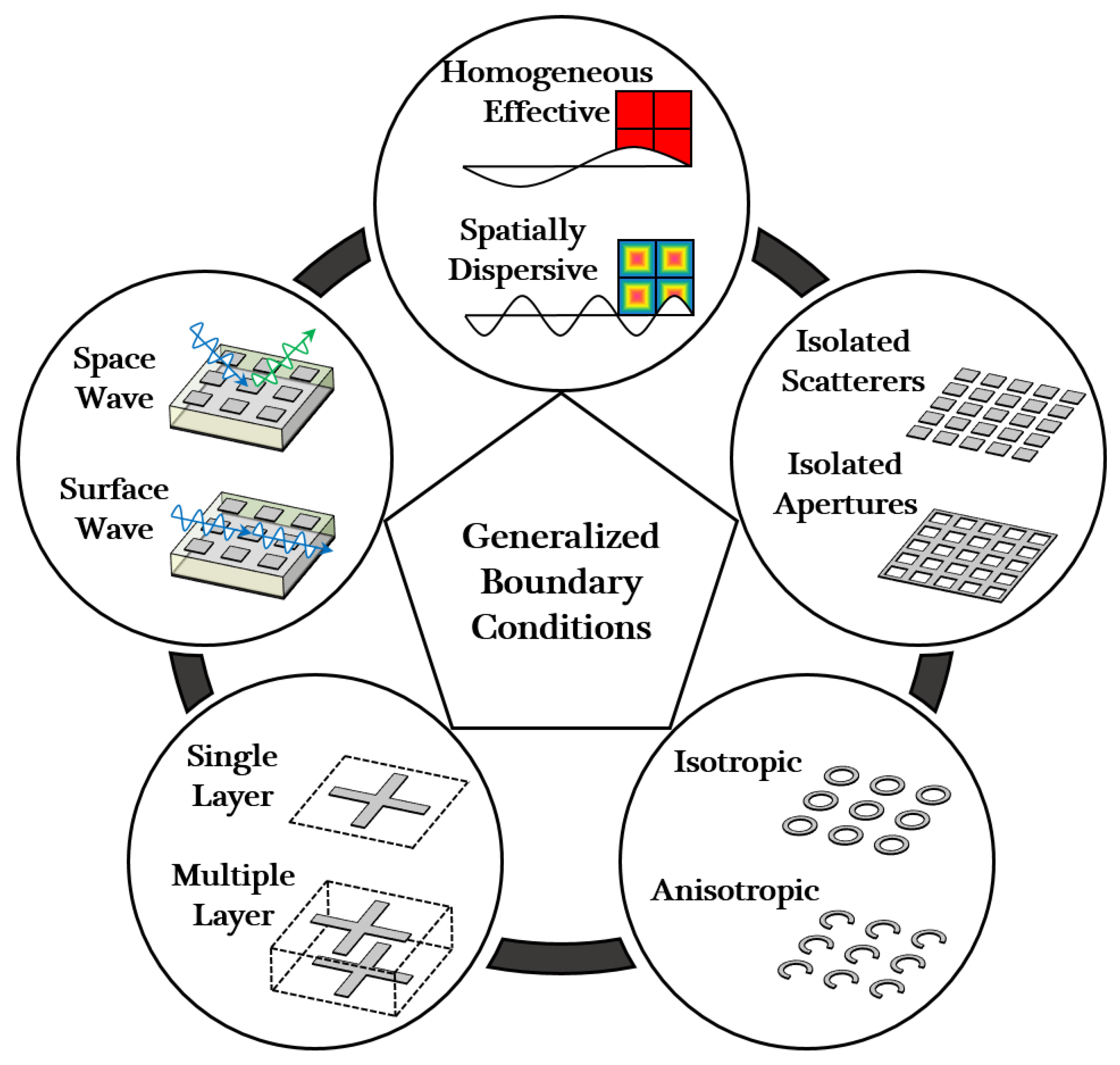
2. Classification of Electromagnetic Surfaces

Most two-dimensional EM surfaces are composed of periodic or quasi-periodic elements, which are also called unit cells. These unit cells have various kinds of features determining the EM properties of surfaces. Five representative features are introduced below, through which the categories of EM surfaces can be described.

2.1. Homogeneous Effective and Spatially Dispersive

Two-dimensional surfaces are always composed of inhomogeneous unit cells, like the periodically distributed square patches shown in Figure 4. However, if the inhomogeneity scale is much smaller than wavelength $\lambda$, the surfaces can be modelled as homogeneous effective mediums [17], whose characteristic parameters are constants along surfaces. Homogeneous effective surfaces whose period, p, is usually much smaller than $\lambda$ can be characterized by effective surface susceptibilities ${\overline{\overline{\chi }}}_{ee}$ and ${\overline{\overline{\chi }}}_{mm}$ [7,21]. As frequency increases, $\lambda$ will gradually become comparable to p, and surfaces cannot be regarded as homogeneous mediums any more. Then ${\overline{\overline{\chi }}}_{ee}$ and ${\overline{\overline{\chi }}}_{mm}$ become functions of space coordinates, and surfaces with wavelength-comparable period are spatially dispersive [17]. FSS is a typical application of spatially dispersive surfaces, whose period is usually designed close to $\lambda /2$.

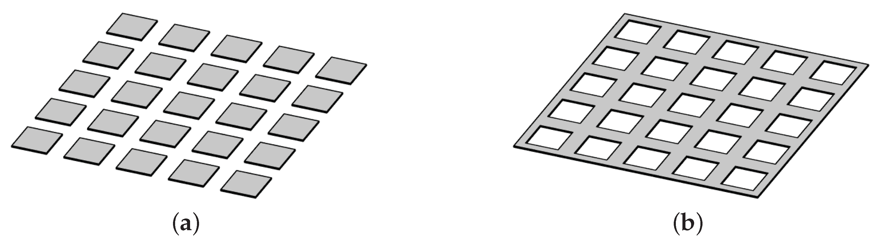
2.2. Isolated Scatterers and Isolated Apertures

Surfaces can also be classified as isolated scatterers or isolated apertures according to their topological structures. Isolated-scatterer surfaces refers to planar arrays composed of separated scatterers, while isolated-aperture surfaces are ones consisting of periodically spaced apertures, as shown in Figure 5. The two surfaces shown in Figure 5 are complementary structures of each other, which are defined as two structures that can cover entire plane without any overlapping. Isolated-scatterer surfaces and isolated-aperture surfaces usually have quite different scattering properties. For example, isolated-scatterer FSS is utilized for designing spatial bandstop filters while isolated-aperture one has characteristic of bandpass [3]. There are also some surfaces that can be either isolated scatterers or isolated apertures, like a grating of parallel conducting wires, which depends on field propagation direction [7].

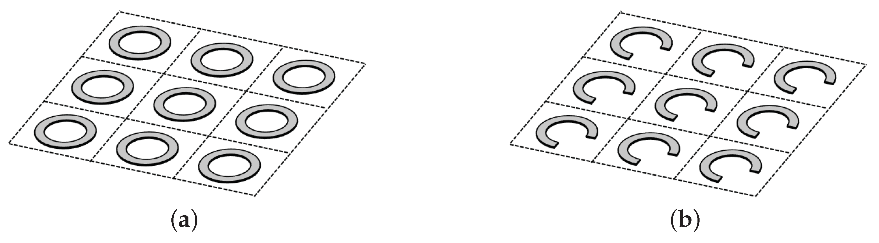
2.3. Isotropic and Anisotropic

In three-dimensional electromagnetics, anisotropy means that the characteristic parameters of mediums are functions of applied field’s direction [22], otherwise they are isotropic. For two-dimensional surfaces, since $\widehat{z}$ dimension is much smaller than $\lambda$, discussion on isotropy and anisotropy do not concern about $\widehat{z}$ component of EM fields. Because isotropic surfaces have the same effects on $\widehat{x}$ and $\widehat{y}$ polarizations, as a result their scattering properties are not related to the azimuthal angle $\phi$ of wave propagation direction $\widehat{k}$, but only to the elevation angle $\theta$. In contrast, anisotropic problems are related to not only $\theta$ but also $\phi$, meanwhile cross-polarization fields may arise in reflection and transmission. An example of isotropic and anisotropic surfaces is given in Figure 6. Actually, there are no purely isotropic surfaces as frequency increases. While $\lambda$ becomes comparable to p, the so-called isotropic problems are also related to $\phi$. That is because even though the scatterers have the same effects on field components along different directions, the periodic square lattice of unit cells is not. As discussed before, at low frequency, p is much smaller than $\lambda$ which makes surfaces effectively homogeneous, and further makes them isotropic.

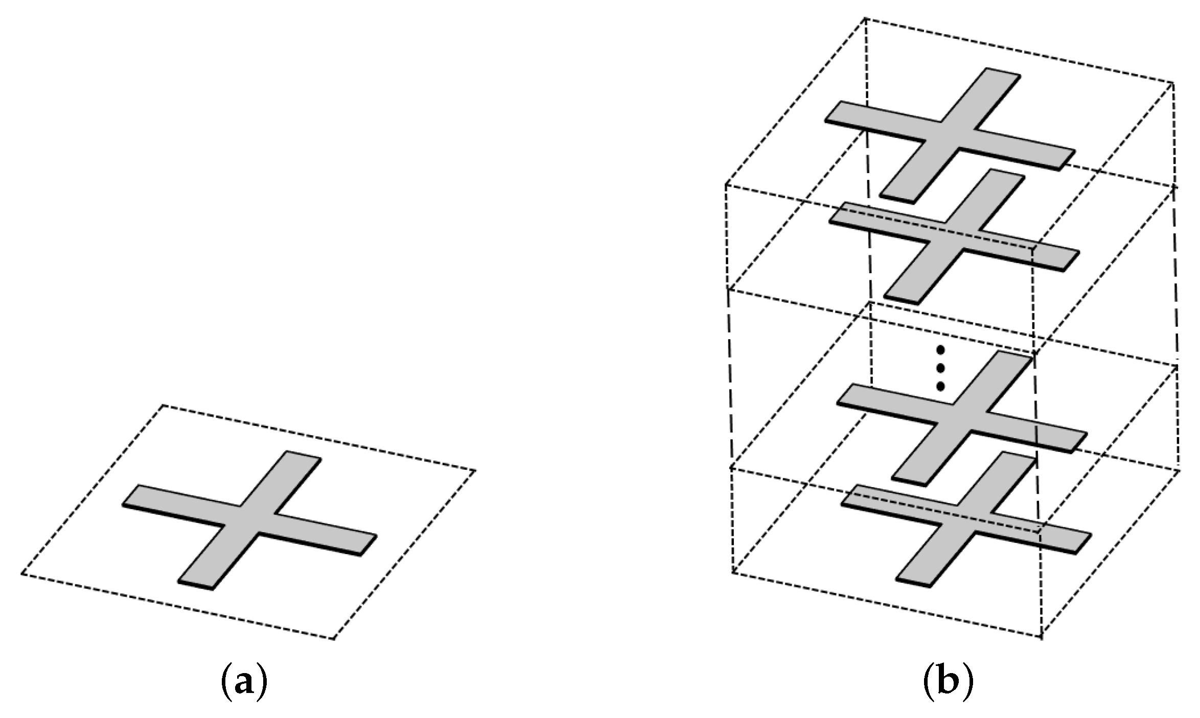
2.4. Single-Layer and Multiple-Layer

When talking about two-dimensional surfaces, we usually refer to single-layer surfaces where $L_z$ is much smaller than $\lambda$, as shown in Figure 7a. However, many desirable properties are realized by cascading multiple layers together like Figure 7b. For instance, multiple-layer surfaces can be utilized to improve bandwidth performance of FSS [3]. Four-layer structures are used to realize a ${360}^{\circ }$ transmission phase range with magnitude larger than –1 dB for FSS-type transmitarray antennas [23]. One feasible solution to problems of multiple-layer structures is to determine surface susceptibilities of each layer and characterize whole structures using equivalent circuit model [24]. Multiple-layer surfaces with a ground plane as bottom layer are called impenetrable surfaces [25], such like EBG and reflectarray antenna [26]. As their name implies, there is no field components below the ground plane of impenetrable surfaces. Conversely, surfaces without bottom ground plane are named as penetrable surfaces, which usually have non-zero transmission like FSS and transmitarray antenna.

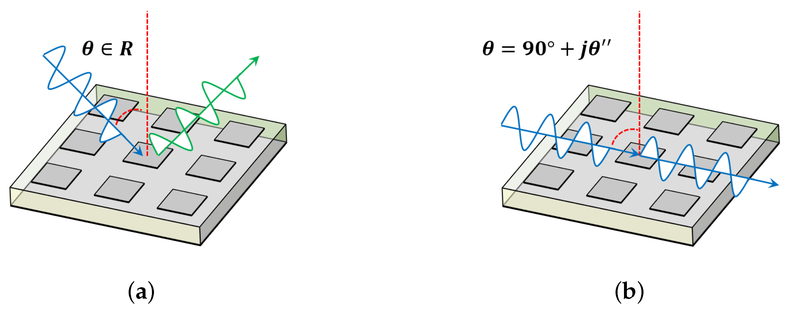
2.5. Space Wave and Surface Wave Features

Two-dimensional surfaces can interact with EM fields of both space-wave modes and surface-wave modes, as shown in Figure 8a. When discussing space-wave modes, it is usually required to characterize reflection and transmission properties of given surfaces. In this case, the propagation constant along the normal direction to the surfaces, $k_z$, is purely real, which means that EM fields can propagate along $\widehat{z}$ direction. Conversely, for surface-wave modes, EM fields would exponentially decay along $\widehat{z}$ direction and $k_z$ is purely imaginary, since fields propagation is constrained along surfaces. Surface-wave modes are eigen propagation modes of given surfaces, where propagation constants of specific frequencies can be determined using eigen-mode solver of commercial simulation softwares like ANSYS High Frequency Structure Simulator (HFSS). Problems related to surface-wave modes can be modelled as special cases of space-wave modes, where incident angle $\theta$ is equal to ${90}^{\circ }$ + $j{\theta }^{″}$. The unknown value of ${\theta }^{″}$ is determined by both surfaces’ characteristic parameters and frequencies. It is worthwhile to point out that there is also a complex mode with complex $k_z$ [27].

2.6. Summary

Five representative features are introduced above to describe different properties of two-dimensional surfaces, each of which can classify surface problems into at least two categories, as shown in Figure 9. If characterization methods corresponding to these features are well established, then GBCs for general surface problems can be further developed. Surface problems related to homogeneous effective, isolated-scatterer, isotropic, single-layer and space-wave mode have been well studied by previous researchers [7,18,21], while others still remain to be solved analytically. In Section 5 and Section 6, characterization methods of isolated-aperture surfaces and surface-wave mode will be discussed respectively, while problems of spatially dispersion, multiple layers, and anisotropy would be discussed in future. Although multiple-layer problems are not specifically discussed in this paper, EM surfaces discussed for surface-wave features in Section 6 are impenetrable ones with ground plane, which are in fact dual-layer structures.

3. Boundary Conditions and Scattering Properties of Two-Dimensional Surfaces

In this section, impedance boundary conditions (IBCs) and generalized sheet transition conditions (GSTCs) will be reviewed first, compared with conventional boundary conditions. Then scattering coefficients of two-dimensional surfaces are defined, and related formulas derived from IBCs and GSTCs are given. Finally, relationship between sheet impedances and surface susceptibilities will be discussed.

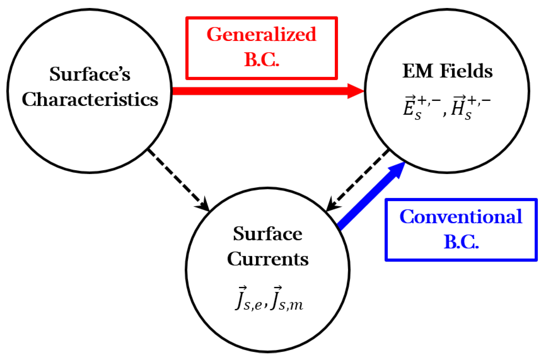
3.1. Evolution of Boundary Conditions

Conventional boundary conditions describe the relationship between field discontinuities across boundary and current sources distributed along boundary, which can be expressed as

$$\widehat{z}\times ({\overrightarrow{H}}_2-{\overrightarrow{H}}_1){{|}_{z=0}={\overrightarrow{J}}_{s,e}|}_{z=0}$$

(1)

$$({\overrightarrow{E}}_2-{\overrightarrow{E}}_1){{|}_{z=0}\times \widehat{z}={\overrightarrow{J}}_{s,m}|}_{z=0},$$

(2)

where $({\overrightarrow{E}}_1,{\overrightarrow{H}}_1)$ and $({\overrightarrow{E}}_2,{\overrightarrow{H}}_2)$ respectively represent the total fields in region z < 0 and z > 0 while ${\overrightarrow{J}}_{s,e}$ and ${\overrightarrow{J}}_{s,m}$ are surface electric and magnetic currents along boundary. Here boundary is selected as the z = 0 plane where EM surfaces are located. If tangential components of $\overrightarrow{E}$ are continuous along the boundary, the magnetic current ${\overrightarrow{J}}_{s,m}$ in Equation (2) would become zero. Similarly, ${\overrightarrow{J}}_{s,e}$ in Equation (1) is equal to zero if tangential magnetic fields are continuous. For general surface problems, both ${\overrightarrow{J}}_{s,e}$ and ${\overrightarrow{J}}_{s,m}$ are non-zero and their values depend on both surfaces’ characteristic parameters and applied EM fields.

The field discontinuities led by EM surfaces can be characterized by their effective sheet impedances, based on which IBCs are derived [15]. The electric sheet impedance ${\overline{\overline{Z}}}_e$ is defined as the ratio of average electric fields ${\overrightarrow{E}}_{\mathrm{av},\tan }$ along surfaces to surface electric current ${\overrightarrow{J}}_{s,e}$ while magnetic sheet impedance ${\overline{\overline{Z}}}_m$ is the ratio of ${\overrightarrow{J}}_{s,m}$ to average magnetic fields ${\overrightarrow{H}}_{\mathrm{av},\tan }$

$${\overrightarrow{E}}_{\mathrm{av},\tan }{{|}_{z=0}={\overline{\overline{Z}}}_e·{\overrightarrow{J}}_{s,e}|}_{z=0}$$

(3)

$${\overrightarrow{H}}_{\mathrm{av},\tan }{{|}_{z=0}={\overline{\overline{Z}}}_m^{-1}·{\overrightarrow{J}}_{s,m}|}_{z=0}.$$

(4)

Based on Equations (1) and (2), surface currents in Equations (3) and (4) can be replaced by the discontinuities of EM fields. Consequently, IBCs describe the relationship between average fields along surfaces and field discontinuities across surfaces

$$\widehat{z}\times ({\overrightarrow{H}}_2-{\overrightarrow{H}}_1){{|}_{z=0}={\overline{\overline{Z}}}_e^{-1}·\frac{1}{2}({\overrightarrow{E}}_{1,\tan }+{\overrightarrow{E}}_{2,\tan })|}_{z=0}$$

(5)

$$({\overrightarrow{E}}_2-{\overrightarrow{E}}_1){{|}_{z=0}\times \widehat{z}={\overline{\overline{Z}}}_m·\frac{1}{2}({\overrightarrow{H}}_{1,\tan }+{\overrightarrow{H}}_{2,\tan })|}_{z=0}.$$

(6)

It is obvious that all field components that appear in IBCs are tangential ones. In general, ${\overline{\overline{Z}}}_e$ and ${\overline{\overline{Z}}}_m$ are two-dimensional tensors. If surfaces are isotropic, the tensorial sheet impedances can be simplified as scalars $Z_e$ and $Z_m$ for specific polarizations.

If EM surfaces are modelled as two-port networks, then the tangential components of $\overrightarrow{E}$ and $\overrightarrow{H}$ can be equivalent to voltage V and current I in circuit theory. As a result, the field relations described by IBCs (Equations (5) and (6)) can be further represented by the bridged-T circuit model [28,29] shown in Figure 10a. The impedance matrix $\left[Z\right]$ [10] of this two-port network can be written as

$$\left[\begin{array}{c}{V}_1\\ V_2\end{array}\right]=\left[\begin{array}{cc}{Z}_e+Z_m/4& Z_e-Z_m/4\\ Z_e-Z_m/4& Z_e+Z_m/4\end{array}\right]\left[\begin{array}{c}{I}_1\\ -I_2\end{array}\right],$$

(7)

where $Z_e$ and $Z_m$ are the sheet impedances defined in Equations (5) and (6). Through the impedance matrix, the S-parameters of the two-port network can be readily computed [10], which stand for the scattering coefficients of EM surfaces that will be discussed in Section 3.2. Consider two special cases:

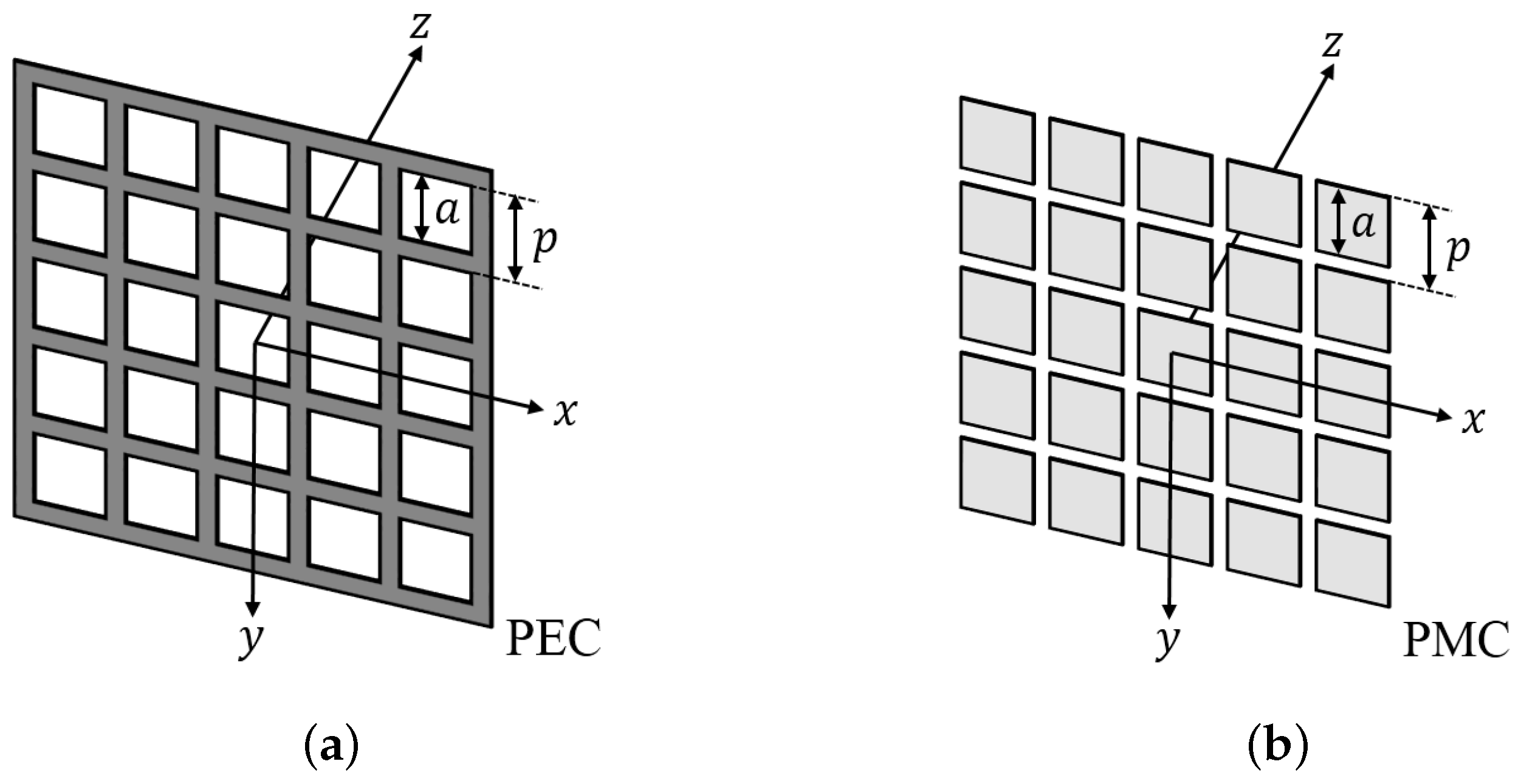
• If the tangential electric fields are continuous across surfaces, the surface magnetic current ${\overrightarrow{J}}_{s,m}$ becomes zero according to Equation (2). As a result, the magnetic impedance $Z_m$ is equal to zero and the bridged-T circuit model can be simplified into a shunt impedance shown in Figure 10b. A specific example is surfaces composed of zero-thickness scatterers made of perfect electric conductor (PEC).
• If the tangential magnetic fields are continuous, then the surface electric current ${\overrightarrow{J}}_{s,e}$ is equal to zero based on Equation (1). Consequently, the electric impedance $Z_e$ would become infinity and the circuit model is simplified as a series impedance shown in Figure 10c. Surfaces made of zero-thickness perfect magnetic conductor (PMC) can be characterized by this model.

The equivalent circuit model can be also utilized to characterize advanced EM surfaces such as perfect electromagnetic conductor (PEMC), which is a generalization of both PEC and PMC with similar properties [30].

With IBCs, field discontinuities led by EM surfaces can be determined once their sheet impedances $Z_e$ and $Z_m$ are known. However, since IBCs only describe the relationship between tangential field components, the values of $Z_e$ and $Z_m$ are sometimes related to the propagation directions and polarizations of applied fields. Thus, they are not characteristic parameters of EM surfaces and their values for different situations cannot be readily determined.

As mentioned in Section 1, the characteristic parameters of two-dimensional surfaces are effective surface susceptibilities, whose values are independent of applied fields. Based on surface susceptibilities, GSTCs are initially derived for metafilms [18], the isolated-scatterer type of metasurfaces [7]. Ignoring the mutually-polarized effects between $({\overrightarrow{P}}_s,{\overrightarrow{M}}_s)$ and $(\overrightarrow{E},\overrightarrow{H})$ [31], where ${\overrightarrow{P}}_s$ and ${\overrightarrow{M}}_s$ are the surface electric and magnetic surface polarization densities respectively, GSTCs for metafilms located in free space can be expressed as

$$\widehat{z}\times ({\overrightarrow{H}}_2-{\overrightarrow{H}}_1){|}_{z=0}=j\omega {\epsilon }_0{\overline{\overline{\chi }}}_{ee}·\frac{1}{2}({\overrightarrow{E}}_{1,\tan }+{\overrightarrow{E}}_{2,\tan }){{|}_{z=0}-\widehat{z}\times {\nabla }_t({\chi }_{mm}^{zz}\frac{1}{2}(H_{1,z}+H_{2,z}))|}_{z=0}$$

(8)

$$({\overrightarrow{E}}_2-{\overrightarrow{E}}_1){|}_{z=0}\times \widehat{z}=j\omega {\mu }_0{\overline{\overline{\chi }}}_{mm}·\frac{1}{2}({\overrightarrow{H}}_{1,\tan }+{\overrightarrow{H}}_{2,\tan }){{|}_{z=0}+\widehat{z}\times {\nabla }_t({\chi }_{ee}^{zz}\frac{1}{2}(E_{1,z}+E_{2,z}))|}_{z=0},$$

(9)

where three-dimensional tensors ${\overline{\overline{\chi }}}_{ee}$ and ${\overline{\overline{\chi }}}_{mm}$ are effective surface electric and magnetic susceptibilities respectively. They are related to the polarizability densities of scatterers per unit area and have unit of meters [7]. For isotropic metafilms, ${\overline{\overline{\chi }}}_{ee}$ and ${\overline{\overline{\chi }}}_{mm}$ become diagonal matrices

$${\overline{\overline{\chi }}}_{ee}=\left[\begin{array}{ccc}{\chi }_{ee}^{xx}& 0& 0\\ 0& {\chi }_{ee}^{yy}& 0\\ 0& 0& {\chi }_{ee}^{zz}\end{array}\right],{\overline{\overline{\chi }}}_{mm}=\left[\begin{array}{ccc}{\chi }_{mm}^{xx}& 0& 0\\ 0& {\chi }_{mm}^{yy}& 0\\ 0& 0& {\chi }_{mm}^{zz}\end{array}\right],$$

(10)

with ${\chi }_{ee}^{xx}$ = ${\chi }_{ee}^{yy}$ and ${\chi }_{mm}^{xx}$ = ${\chi }_{mm}^{yy}$. Thus, there are four unknown terms in total in surface susceptibilities of isotropic problems. Through GSTCs, field relations across metafilms can be analytically determined once ${\overline{\overline{\chi }}}_{ee}$ and ${\overline{\overline{\chi }}}_{mm}$ are known. An overview of characterizing metafilms using GSTCs and its related applications in metasurfaces design is given in [7], including waveguide design [32] and guided wave characterization [27]. Numerical methods based on GSTCs are also derived from Equations (8) and (9) [33,34,35]. However, the surface characterization method based on surface susceptibilities and GSTCs are only appropriate for single-layer metafilms [18]. For EM surfaces with other types of features like isolated aperture or multiple layers, the corresponding characterization methods remain to be explored.

Since neither IBCs nor GSTCs can give a general solution to surface problems, it is necessary to derive generalized boundary conditions (GBCs) with characteristic parameters ${\overline{\overline{\chi }}}_{ee}$ and ${\overline{\overline{\chi }}}_{mm}$, based on which the field discontinuities across different kinds of EM surfaces can be analytically characterized. The mathematical model of GBCs can be generalized as

$$F({\overrightarrow{E}}_1,{\overrightarrow{E}}_2,{\overrightarrow{H}}_1,{\overrightarrow{H}}_2,{\overline{\overline{\chi }}}_{ee},{\overline{\overline{\chi }}}_{mm})=0.$$

(11)

Once ${\overline{\overline{\chi }}}_{ee}$ and ${\overline{\overline{\chi }}}_{mm}$ of given surfaces are determined, their scattering properties can be readily computed by analytically solving Equation (11). In Section 5 and Section 6, the mathematical model F for problems of isolated aperture and surface-wave mode will be derived respectively.

3.2. Scattering Properties of Two-Dimensional Surfaces

Scattering properties of periodic EM surfaces are usually characterized by reflection and transmission coefficients, which describe the field relations between incidence, reflection and transmission, under plane-wave incidence. Here it is assumed that EM surfaces are located along z = 0 in free space and incident plane wave illuminates the surfaces from region z < 0. Thus $({\overrightarrow{E}}_1,{\overrightarrow{H}}_1)$ in region z < 0 are the superposition of incident field (${\overrightarrow{E}}_i$, ${\overrightarrow{H}}_i$) and reflected fields (${\overrightarrow{E}}_r$, ${\overrightarrow{H}}_r$) while $({\overrightarrow{E}}_2,{\overrightarrow{H}}_2)$ in region z > 0 are equal to transmitted fields (${\overrightarrow{E}}_t$, ${\overrightarrow{H}}_t$) only. Since it is free space on both sides of surfaces and the phase discontinuities led by periodic structures are same everywhere, the incident, reflected and transmitted angles should be equal to each other according to phase matching. Then the wave vectors of incidence, reflection and transmission can be respectively expressed as

$$\begin{array}{c}{\overrightarrow{k}}_i=k_0(\widehat{x}sin\theta cos\phi +\widehat{y}sin\theta sin\phi +\widehat{z}cos\theta )\end{array}$$

(12a)

$$\begin{array}{c}{\overrightarrow{k}}_r=k_0(\widehat{x}sin\theta cos\phi +\widehat{y}sin\theta sin\phi -\widehat{z}cos\theta )\end{array}$$

(12b)

$$\begin{array}{c}{\overrightarrow{k}}_t=k_0(\widehat{x}sin\theta cos\phi +\widehat{y}sin\theta sin\phi +\widehat{z}cos\theta ),\end{array}$$

(12c)

where $k_0$ = $\omega \sqrt{{\epsilon }_0{\mu }_0}$ is the wavenumber in free space.

For simplicity, only isotropic surfaces are discussed here. As mentioned in Section 2.3, scattering properties of isotropic surfaces are independent of the azimuth angle $\phi$. Thus $\phi$ is set as $0^{\circ }$ in the following derivations. With the assumption of isotropy, the TE-polarized fields can be expressed as [22]

$$\begin{array}{c}{\overrightarrow{E}}_i^{\mathrm{TE}}=\widehat{y}{E}_0{e}^{-j{\overrightarrow{k}}_i·\overrightarrow{r}}\end{array}$$

(13a)

$$\begin{array}{c}{\overrightarrow{E}}_r^{\mathrm{TE}}=\widehat{y}{\Gamma }^{\mathrm{TE}}{E}_0{e}^{-j{\overrightarrow{k}}_r·\overrightarrow{r}}\end{array}$$

(13b)

$$\begin{array}{c}{\overrightarrow{E}}_t^{\mathrm{TE}}=\widehat{y}{T}^{\mathrm{TE}}{E}_0{e}^{-j{\overrightarrow{k}}_t·\overrightarrow{r}}\end{array}$$

(13c)

$$\begin{array}{c}{\overrightarrow{H}}_i^{\mathrm{TE}}=(-\widehat{x}cos\theta +\widehat{z}sin\theta )E_0{e}^{-j{\overrightarrow{k}}_i·\overrightarrow{r}}/{\eta }_0\end{array}$$

(13d)

$$\begin{array}{c}{\overrightarrow{H}}_r^{\mathrm{TE}}=(\widehat{x}cos\theta +\widehat{z}sin\theta ){\Gamma }^{\mathrm{TE}}{E}_0{e}^{-j{\overrightarrow{k}}_r·\overrightarrow{r}}/{\eta }_0\end{array}$$

(13e)

$$\begin{array}{c}{\overrightarrow{H}}_t^{\mathrm{TE}}=(-\widehat{x}cos\theta +\widehat{z}sin\theta )T^{\mathrm{TE}}{E}_0{e}^{-j{\overrightarrow{k}}_t·\overrightarrow{r}}/{\eta }_0,\end{array}$$

(13f)

and for TM polarization

$$\begin{array}{c}{\overrightarrow{E}}_i^{\mathrm{TM}}=(-\widehat{x}cos\theta +\widehat{z}sin\theta )E_0{e}^{-j{\overrightarrow{k}}_i·\overrightarrow{r}}\end{array}$$

(14a)

$$\begin{array}{c}{\overrightarrow{E}}_r^{\mathrm{TM}}=(-\widehat{x}cos\theta -\widehat{z}sin\theta ){\Gamma }^{\mathrm{TM}}{E}_0{e}^{-j{\overrightarrow{k}}_r·\overrightarrow{r}}\end{array}$$

(14b)

$$\begin{array}{c}{\overrightarrow{E}}_t^{\mathrm{TM}}=(-\widehat{x}cos\theta +\widehat{z}sin\theta )T^{\mathrm{TM}}{E}_0{e}^{-j{\overrightarrow{k}}_t·\overrightarrow{r}}\end{array}$$

(14c)

$$\begin{array}{c}{\overrightarrow{H}}_i^{\mathrm{TM}}=-\widehat{y}{E}_0{e}^{-j{\overrightarrow{k}}_i·\overrightarrow{r}}/{\eta }_0\end{array}$$

(14d)

$$\begin{array}{c}{\overrightarrow{H}}_r^{\mathrm{TM}}=\widehat{y}{\Gamma }^{\mathrm{TM}}{E}_0{e}^{-j{\overrightarrow{k}}_r·\overrightarrow{r}}/{\eta }_0\end{array}$$

(14e)

$$\begin{array}{c}{\overrightarrow{H}}_t^{\mathrm{TM}}=-\widehat{y}{T}^{\mathrm{TM}}{E}_0{e}^{-j{\overrightarrow{k}}_t·\overrightarrow{r}}/{\eta }_0,\end{array}$$

(14f)

where $\overrightarrow{r}=x\widehat{x}+y\widehat{y}+z\widehat{z}$ and ${\eta }_0=\sqrt{{\mu }_0/{\epsilon }_0}$ is the wave impedance in free space. $\Gamma$ and T represent reflection and transmission coefficients respectively.

According to Equations (13) and (14), if the tangential components of $\overrightarrow{E}$ are continuous along surfaces, for instance, surfaces composed of zero-thickness PEC scatterers, then $\Gamma$ and T satisfy that

$$1+\Gamma =T.$$

(15)

Under this condition, once either $\Gamma$ or T is determined, the other one can be easily computed through Equation (15).

Similarly, if tangential magnetic fields are continuous, like periodic zero-thickness PMC scatterers, then

$$\Gamma +T=1.$$

(16)

It should be noted that Equations (15) and (16) are only valid under condition that the discussed surfaces are located in free space. For example, if either side of surfaces is filled with dielectric materials, the corresponding relations for TM polarization need to be modified according to the reflected and transmitted angles.

3.3. Relations between Scattering Properties and Sheet Impedances

Since field relations across surfaces can be described by IBCs, their scattering coefficients can be determined from sheet impedances. By substituting the EM field expressions (Equations (13) and (14)) into IBCs (Equations (5) and (6)), $\Gamma$ and T of isotropic EM surfaces can be written as functions of $Z_e$ and $Z_m$ as

$$\begin{array}{c}{\Gamma }^{\mathrm{TE}}(\theta )=\frac{Z_e^{\mathrm{TE}}(\theta )Z_m^{\mathrm{TE}}(\theta )-{({\eta }_0/cos\theta )}^2}{(2Z_e^{\mathrm{TE}}(\theta )+{\eta }_0/cos\theta )(\frac{1}{2}{Z}_m^{\mathrm{TE}}(\theta )+{\eta }_0/cos\theta )}\end{array}$$

(17a)

$$\begin{array}{c}{T}^{\mathrm{TE}}(\theta )=\frac{({\eta }_0/cos\theta )(2Z_e^{\mathrm{TE}}(\theta )-\frac{1}{2}{Z}_n^{\mathrm{TE}}(\theta ))}{(2Z_e^{\mathrm{TE}}(\theta )+{\eta }_0/cos\theta )(\frac{1}{2}{Z}_m^{\mathrm{TE}}(\theta )+{\eta }_0/cos\theta )},\end{array}$$

(17b)

$$\begin{array}{c}{\Gamma }^{\mathrm{TM}}(\theta )=\frac{Z_e^{\mathrm{TM}}(\theta )Z_m^{\mathrm{TM}}(\theta )-{({\eta }_{0}cos\theta )}^2}{(2Z_e^{\mathrm{TM}}(\theta )+{\eta }_{0}cos\theta )(\frac{1}{2}{Z}_m^{\mathrm{TM}}(\theta )+{\eta }_{0}cos\theta )}\end{array}$$

(18a)

$$\begin{array}{c}{T}^{\mathrm{TM}}(\theta )=\frac{({\eta }_{0}cos\theta )(2Z_e^{\mathrm{TM}}(\theta )-\frac{1}{2}{Z}_m^{\mathrm{TM}}(\theta ))}{(2Z_e^{\mathrm{TM}}(\theta )+{\eta }_{0}cos\theta )(\frac{1}{2}{Z}_m^{\mathrm{TM}}(\theta )+{\eta }_{0}cos\theta )},\end{array}$$

(18b)

for TE and TM polarizations respectively. Through Equations (17) and (18), the scattering coefficients for arbitrary incident angles and polarizations can be readily computed if the corresponding sheet impedances are known. By rewriting Equations (17) and (18), $Z_e$ and $Z_m$ can be expressed in terms of $\Gamma$ and T, through which the sheet impedances of given surfaces can be extracted from the corresponding measured or simulated scattering coefficients. However, as mentioned before, the values of sheet impedances are related to the properties of applied fields. The values of $Z_e$ and $Z_m$ extracted from one situation cannot be utilized to compute scattering coefficients of others with different incident angle $\theta$ or polarizations (TE/TM).

As discussed before, for surfaces composed of zero-thickness PEC scatterers, the tangential electric fields are continuous and the magnetic sheet impedance $Z_m$ is equal to zero. Then Equations (17) and (18) can be simplified as

$$\begin{array}{c}{\Gamma }_e^{\mathrm{TE}}(\theta )=-\frac{{\eta }_0}{2Z_e^{\mathrm{TE}}(\theta )cos\theta }/(1+\frac{{\eta }_0}{2Z_e^{\mathrm{TE}}(\theta )cos\theta })\end{array}$$

(19a)

$$\begin{array}{c}{T}_e^{\mathrm{TE}}(\theta )=1/(1+\frac{{\eta }_0}{2Z_e^{\mathrm{TE}}(\theta )cos\theta }),\end{array}$$

(19b)

and

$$\begin{array}{c}{\Gamma }_e^{\mathrm{TM}}(\theta )=-\frac{{\eta }_{0}cos\theta }{2Z_e^{\mathrm{TM}}(\theta )}/(1+\frac{{\eta }_{0}cos\theta }{2Z_e^{\mathrm{TM}}(\theta )})\end{array}$$

(20a)

$$\begin{array}{c}{T}_e^{\mathrm{TM}}(\theta )=1/(1+\frac{{\eta }_{0}cos\theta }{2Z_e^{\mathrm{TM}}(\theta )}),\end{array}$$

(20b)

which satisfy the relation shown in Equation (15). Similarly, expressions of $\Gamma$ and T for surfaces composed of zero-thickness PMC scatterers can be derived by letting $Z_e$ = ∞.

3.4. Relations between Scattering Properties and Surface Susceptibilities

The scattering coefficients of EM surfaces can also be determined from surface susceptibilities through the field relations defined by GSTCs. By substituting EM field expressions (Equations (13) and (14)) into GSTCs (Equations (8) and (9)), $\Gamma$ and T can be written as functions of ${\overline{\overline{\chi }}}_{ee}$ and ${\overline{\overline{\chi }}}_{mm}$ [7]

$$\begin{array}{c}{\Gamma }^{\mathrm{TE}}(\theta )=\frac{-j\frac{k_0}{2cos\theta }({\chi }_{ee}^{yy}-{\chi }_{mm}^{xx}{cos}^2\theta +{\chi }_{mm}^{zz}{sin}^2\theta )}{1-{(\frac{k_0}{2})}^2{\chi }_{mm}^{xx}({\chi }_{ee}^{yy}+{\chi }_{mm}^{zz}{sin}^2\theta )+j\frac{k_0}{2cos\theta }({\chi }_{ee}^{yy}+{\chi }_{mm}^{xx}{cos}^2\theta +{\chi }_{mm}^{zz}{sin}^2\theta )}\end{array}$$

(21a)

$$\begin{array}{c}{T}^{\mathrm{TE}}(\theta )=\frac{1+{(\frac{k_0}{2})}^2{\chi }_{mm}^{xx}({\chi }_{ee}^{yy}+{\chi }_{mm}^{zz}{sin}^2\theta )}{1-{(\frac{k_0}{2})}^2{\chi }_{mm}^{xx}({\chi }_{ee}^{yy}+{\chi }_{mm}^{zz}{sin}^2\theta )+j\frac{k_0}{2cos\theta }({\chi }_{ee}^{yy}+{\chi }_{mm}^{xx}{cos}^2\theta +{\chi }_{mm}^{zz}{sin}^2\theta )},\end{array}$$

(21b)

and

$$\begin{array}{c}{\Gamma }^{\mathrm{TM}}(\theta )=\frac{-j\frac{k_0}{2cos\theta }(-{\chi }_{mm}^{yy}+{\chi }_{ee}^{xx}{cos}^2\theta -{\chi }_{ee}^{zz}{sin}^2\theta )}{1-{(\frac{k_0}{2})}^2{\chi }_{ee}^{xx}({\chi }_{mm}^{yy}+{\chi }_{ee}^{zz}{sin}^2\theta )+j\frac{k_0}{2cos\theta }({\chi }_{mm}^{yy}+{\chi }_{ee}^{xx}{cos}^2\theta +{\chi }_{ee}^{zz}{sin}^2\theta )}\end{array}$$

(22a)

$$\begin{array}{c}{T}^{\mathrm{TM}}(\theta )=\frac{1+{(\frac{k_0}{2})}^2{\chi }_{ee}^{xx}({\chi }_{mm}^{yy}+{\chi }_{ee}^{zz}{sin}^2\theta )}{1-{(\frac{k_0}{2})}^2{\chi }_{ee}^{xx}({\chi }_{mm}^{yy}+{\chi }_{ee}^{zz}{sin}^2\theta )+j\frac{k_0}{2cos\theta }({\chi }_{mm}^{yy}+{\chi }_{ee}^{xx}{cos}^2\theta +{\chi }_{ee}^{zz}{sin}^2\theta )},\end{array}$$

(22b)

for TE and TM polarizations respectively. Through Equations (21) and (22), $\Gamma$ and T for arbitrary incident conditions can be analytically computed once ${\overline{\overline{\chi }}}_{ee}$ and ${\overline{\overline{\chi }}}_{mm}$ are determined. Different from sheet impedances, surface susceptibilities are characteristic parameters of surfaces that do not vary with properties of applied fields. Thus, ${\overline{\overline{\chi }}}_{ee}$ and ${\overline{\overline{\chi }}}_{mm}$ extracted from one situation can be directly utilized in the computation of others. The extraction method of surface susceptibilities from limited sets of full-wave simulations will be discussed in Section 4.1.

Consider surfaces composed of isotropic zero-thickness PEC scatterers again. Since transverse magnetic current cannot exist along PEC surfaces, the values of ${\chi }_{mm}^{xx}$ and ${\chi }_{mm}^{yy}$ should be equal to zero. Meanwhile, ${\chi }_{ee}^{zz}$ is also equal to zero because there is no electric current along z-direction due to zero thickness. ${\chi }_{ee}^{xx}$ and ${\chi }_{ee}^{yy}$ are non-zero due to the induced electric currents along PEC surface. Also, there are electric current loops formed along surfaces when the incident angle $\theta$ is not equal to zero, leading to the non-zero ${\chi }_{mm}^{zz}$. Therefore, for this special case, surface susceptibilities can be simplified as

$${\overline{\overline{\chi }}}_{ee}=\left[\begin{array}{ccc}{\chi }_{ee}^{xx}& 0& 0\\ 0& {\chi }_{ee}^{yy}& 0\\ 0& 0& 0\end{array}\right],{\overline{\overline{\chi }}}_{mm}=\left[\begin{array}{ccc}0& 0& 0\\ 0& 0& 0\\ 0& 0& {\chi }_{mm}^{zz}\end{array}\right],$$

(23)

with ${\chi }_{ee}^{xx}$ = ${\chi }_{ee}^{yy}$. There are only two unknowns to be determined. Then Equations (21) and (22), which compute scattering coefficients based on surface susceptibilities, can be respectively simplified as

$$\begin{array}{c}{\Gamma }_e^{\mathrm{TE}}(\theta )=\frac{-j\frac{k_0}{2cos\theta }({\chi }_{ee}^{yy}+{\chi }_{mm}^{zz}{sin}^2\theta )}{1+j\frac{k_0}{2cos\theta }({\chi }_{ee}^{yy}+{\chi }_{mm}^{zz}{sin}^2\theta )}\end{array}$$

(24a)

$$\begin{array}{c}{T}_e^{\mathrm{TE}}(\theta )=\frac{1}{1+j\frac{k_0}{2cos\theta }({\chi }_{ee}^{yy}+{\chi }_{mm}^{zz}{sin}^2\theta )},\end{array}$$

(24b)

and

$$\begin{array}{c}{\Gamma }_e^{\mathrm{TM}}(\theta )=\frac{-j\frac{k_0}{2}{\chi }_{ee}^{xx}cos\theta }{1+j\frac{k_0}{2}{\chi }_{ee}^{xx}cos\theta }\end{array}$$

(25a)

$$\begin{array}{c}{T}_e^{\mathrm{TM}}(\theta )=\frac{1}{1+j\frac{k_0}{2}{\chi }_{ee}^{xx}cos\theta }.\end{array}$$

(25b)

The corresponding results for zero-thickness surfaces composed of PMC scatterers can be derived using a similar procedure by letting ${\chi }_{ee}^{xx}$, ${\chi }_{ee}^{yy}$ and ${\chi }_{mm}^{zz}$ equal to zero.

3.5. Relations between Sheet Impedances and Surface Susceptibilities

Two-dimensional periodic surfaces can be represented by either sheet impedances or surface susceptibilities, both of which can be utilized to characterize scattering properties of surfaces analytically. Using sheet impedances, EM surfaces are equivalent to the circuit models shown in Figure 10, based on which more complicated surface problems like multiple layers can be solved through cascading network. However, the values of sheet impedances are related to the properties of applied fields, which makes it difficult to determine $Z_e$ and $Z_m$ for arbitrary incident angles and polarizations. Surface susceptibilities are characteristic parameters that do not vary with the applied field, thus their values can be determined through limited sets of $(\Gamma ,T)$ and then be utilized to compute scattering coefficients for arbitrary situations through the field relations described by GSTCs. But GSTCs are only appropriate for metasurfaces with single-layer structures, implying that it cannot be directly utilized to solve problems of multiple layers. Thus, here it is proposed to combine sheet impedances and surface susceptibilities together in order to solve more complicated surface problems. Once surface susceptibilities of given surfaces are determined, the corresponding sheet impedances for arbitrary incident angles and polarizations can be readily computed and utilized for surface characterizations.

Take the TE polarization as an example. Based on the EM field expressions of TE polarization (Equation (13)), GSTCs can be rewritten as

$$\widehat{z}\times ({\overrightarrow{H}}_2-{\overrightarrow{H}}_1){{|}_{z=0}=j\frac{k_0}{{\eta }_0}({\chi }_{ee}^{yy}+{\chi }_{mm}^{zz}{sin}^2\theta )\frac{1}{2}({\overrightarrow{E}}_{1,\tan }+{\overrightarrow{E}}_{2,\tan })|}_{z=0}$$

(26)

$$({\overrightarrow{E}}_2-{\overrightarrow{E}}_1){{|}_{z=0}\times \widehat{z}=j{\eta }_0{k}_0{\chi }_{mm}^{xx}\frac{1}{2}({\overrightarrow{H}}_{1,\tan }+{\overrightarrow{H}}_{2,\tan })|}_{z=0}.$$

(27)

By comparing Equations (26) and (27) with IBCs (Equations (5) and (6)), relations between sheet impedances and surface susceptibilities can be written as

$$Z_e^{\mathrm{TE}}(\theta )=-\frac{j{\eta }_0}{k_0({\chi }_{ee}^{yy}+{\chi }_{mm}^{zz}{sin}^2\theta )}$$

(28)

$$Z_m^{\mathrm{TE}}(\theta )=j{\eta }_0{k}_0{\chi }_{mm}^{xx},$$

(29)

where $Z_e$ and $Z_m$ are the impedance shown in Figure 10a. It is obvious that for TE polarization $Z_e$ is related to the incident angle $\theta$ while $Z_m$ is $\theta$-independent. Similarly, for TM polarization, the corresponding relations can be written as

$$Z_e^{\mathrm{TM}}(\theta )=-\frac{j{\eta }_0}{k_0{\chi }_{ee}^{xx}}$$

(30)

$$Z_m^{\mathrm{TM}}(\theta )=j{\eta }_0{k}_0({\chi }_{mm}^{yy}+{\chi }_{ee}^{zz}{sin}^2\theta ),$$

(31)

where $Z_e$ is $\theta$-independent but $Z_m$ is not. Therefore, the values of $Z_e$ and $Z_m$ for arbitrary incident angles and polarizations can be readily computed through Equations (28)–(31), once ${\overline{\overline{\chi }}}_{ee}$ and ${\overline{\overline{\chi }}}_{mm}$ of given surfaces are determined.

For arbitrary single-layer isotropic metafilms, their surface susceptibilities can be extracted using the method that will be introduced in Section 4.1. With surface susceptibilities determined, the scattering coefficients for arbitrary incident angles and polarizations can be readily computed through Equations (21) and (22). Meanwhile, the corresponding sheet impedances can be determined through Equations (28)–(31), which can be further utilized to solve more complicated problems with equivalent circuit model and impedance matrix. While the characterization method described above is only valid for metafilms with isolated-scatterer topological structures, the corresponding method for metascreens composed of periodic isolated apertures will be derived in Section 5. Also, the combination of sheet impedances and surface susceptibilities will be utilized in Section 6 for characterizing surface-wave mode of multiple-layer impenetrable surfaces.

4. Surface Characterizations Based on Surface Susceptibilities

In Section 3, it is shown that scattering coefficients of EM surfaces for arbitrary $\theta$ and polarizations can be analytically computed through Equations (21) and (22) once surface susceptibilities are determined. This section will present how to extract surface susceptibilities of given surfaces from limited sets of unit cell simulations and show the procedure of surface characterizations based on surface susceptibilities. In order to make related formulas shown in Section 3 applicable, it is assumed that the surfaces discussed here are single-layer isotropic metafilms which have period of unit cells much smaller than wavelength and are composed of periodic isolated scatterers.

4.1. Extraction of Surface Susceptibilities

According to Equation (10) and related discussions, there are totally four unknown components of surface susceptibilities for isotropic problems. Since surface susceptibilities are characteristic parameters that do not vary with properties of applied fields, their values can be determined from $\Gamma$ and T with different incident angles and polarizations. Derived from Equations (21) and (22), the surface susceptibilities can be extracted through [7]

$$\begin{array}{c}{\chi }_{ee}^{xx}={\chi }_{ee}^{yy}=\frac{2j}{k_0}\frac{\Gamma (0^{\circ })+T(0^{\circ })-1}{\Gamma (0^{\circ })+T(0^{\circ })+1}\end{array}$$

(32a)

$$\begin{array}{c}{\chi }_{mm}^{xx}={\chi }_{mm}^{yy}=\frac{2j}{k_0}\frac{\Gamma (0^{\circ })-T(0^{\circ })+1}{\Gamma (0^{\circ })-T(0^{\circ })-1}\end{array}$$

(32b)

$$\begin{array}{c}{\chi }_{ee}^{zz}=-\frac{{\chi }_{mm}^{yy}}{{sin}^2{\theta }_0}+\frac{2jcos{\theta }_0}{k_0{sin}^2{\theta }_0}\frac{{\Gamma }^{\mathrm{TM}}({\theta }_0)-T^{\mathrm{TM}}({\theta }_0)+1}{{\Gamma }^{\mathrm{TM}}({\theta }_0)-T^{\mathrm{TM}}({\theta }_0)-1}\end{array}$$

(32c)

$$\begin{array}{c}{\chi }_{mm}^{zz}=-\frac{{\chi }_{ee}^{yy}}{{sin}^2{\theta }_0}+\frac{2jcos{\theta }_0}{k_0{sin}^2{\theta }_0}\frac{{\Gamma }^{\mathrm{TE}}({\theta }_0)+T^{\mathrm{TE}}({\theta }_0)-1}{{\Gamma }^{\mathrm{TE}}({\theta }_0)+T^{\mathrm{TE}}({\theta }_0)+1},\end{array}$$

(32d)

where $\Gamma (0^{\circ })$, $T(0^{\circ })$, $\Gamma ({\theta }_0)$ and $T({\theta }_0)$ stand for the reflection and transmission coefficients of normal incidence and oblique incidence with $\theta$ = ${\theta }_0$ respectively. It is worthwhile to point out that isotropic surfaces have same scattering coefficients $\Gamma (0^{\circ })$ and $T(0^{\circ })$ of normal incidence for TE and TM polarizations. The values of $\Gamma$ and T can be obtained through either measurements of periodic surfaces or full-wave simulations of unit cells with periodic boundary conditions (PBCs), while the simulation method is utilized in this paper. According to Equation (32), three sets of simulations are required to determine the values of ${\overline{\overline{\chi }}}_{ee}$ and ${\overline{\overline{\chi }}}_{mm}$:

• one simulation of normal incidence with $\theta$ = $0^{\circ }$ to obtain $\Gamma (0^{\circ })$ and $T(0^{\circ })$;
• one simulation of TE-polarized oblique incidence with $\theta$ = ${\theta }_0$ to obtain ${\Gamma }^{\mathrm{TE}}({\theta }_0)$ and $T^{\mathrm{TE}}({\theta }_0)$;
• one simulation of TM-polarized oblique incidence with $\theta$ = ${\theta }_0$ to obtain ${\Gamma }^{\mathrm{TM}}({\theta }_0)$ and $T^{\mathrm{TM}}({\theta }_0)$.

4.2. Surface Characterization Procedure

Once ${\overline{\overline{\chi }}}_{ee}$ and ${\overline{\overline{\chi }}}_{mm}$ are determined, $\Gamma$ and T for arbitrary applied fields can be readily computed through Equations (21) and (22). For given single-layer isotropic metafilms, the characterization procedure based on surface susceptibilities is listed below:

• carry out three sets of unit cell simulations of given surfaces, including $\theta$ = $0^{\circ }$ and $\theta$ = ${\theta }_0$ for both TE and TM polarizations;
• extract ${\overline{\overline{\chi }}}_{ee}$ and ${\overline{\overline{\chi }}}_{mm}$ from simulated scattering coefficients through Equation (32);
• compute $(\Gamma ,T)$ for arbitrary $\theta$ and polarizations using Equations (21) and (22).

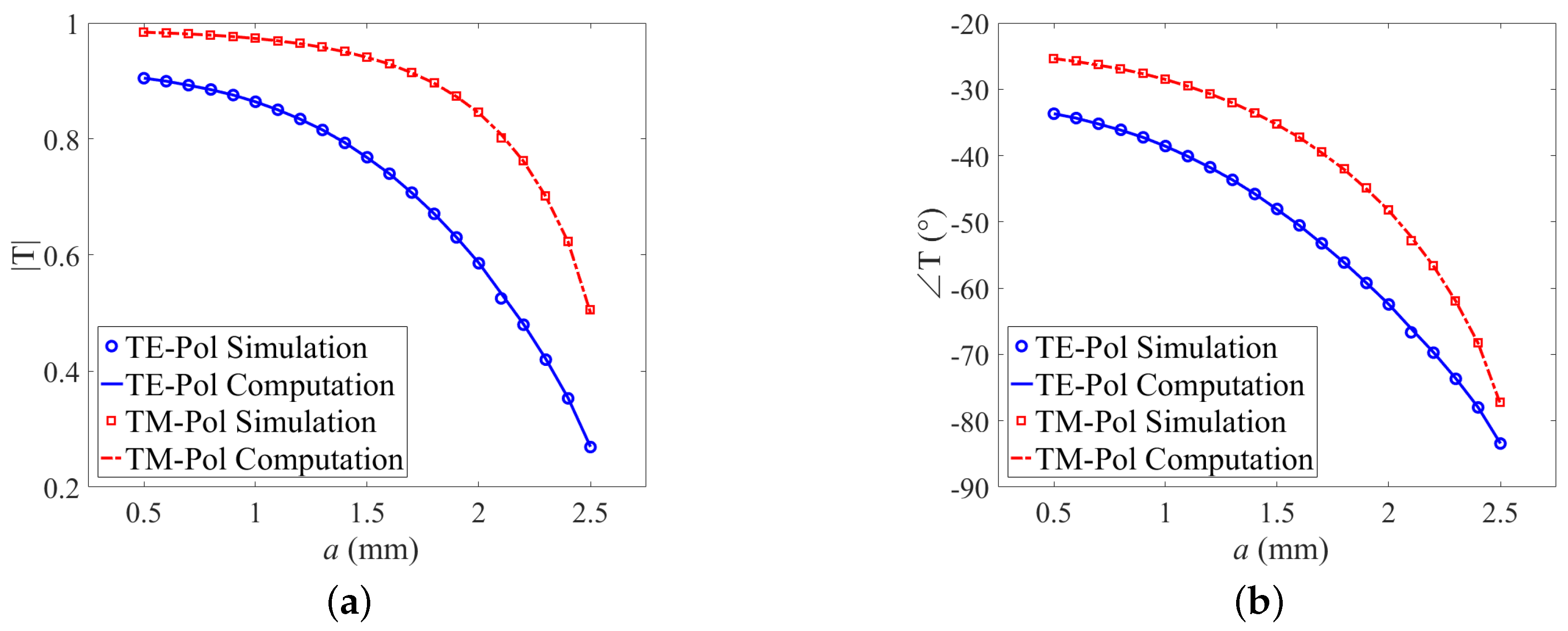
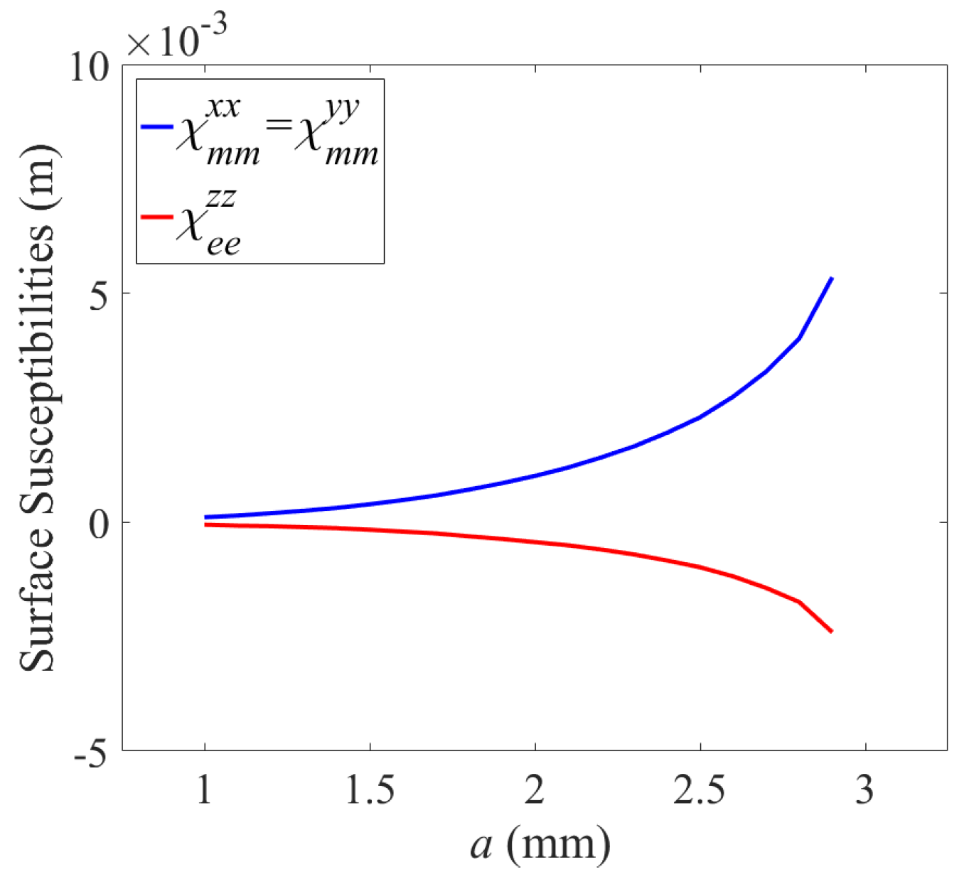
4.3. Example of Surface Characterizations Based on Surface Susceptibilities

An example of surface characterization based on surface susceptibilities is given here. Configuration of the discussed surface’s unit cell is shown in Figure 11, which is composed of dual-layer PEC Jerusalem cross-shaped patches with four metallized vertical vias. Its scattering properties at 10 GHz will be characterized through the procedure introduced above. At 10 GHz, the wavelength $\lambda$ is equal to 30 mm, which is much larger than unit cell’s period p, which makes the assumption of homogeneous effective valid. Also, its thickness h is much smaller than p, so it can be regarded as a single-layer structure. The unit cell has the same effect on EM fields along $\widehat{x}$ and $\widehat{y}$ directions, leading to isotropy of the discussed surface.

In order to determine its surface susceptibilities, three simulations of the unit cell are done at 10 GHz using ANSYS HFSS with PBCs, where the value of ${\theta }_0$ is selected as ${60}^{\circ }$. The extracted surface susceptibilities based on Equation (32) with variation of parameter a are shown in Figure 12. The fluctuation of ${\chi }_{mm}^{zz}$ should be due to the numerical errors from simulation software.

With ${\overline{\overline{\chi }}}_{ee}$ and ${\overline{\overline{\chi }}}_{mm}$ determined, $\Gamma$ and T of this surface for arbitrary $\theta$ and polarizations can be readily computed. For verification purpose, computations with $\theta$ = ${45}^{\circ }$ for both TE and TM polarizations are selected as examples. Figure 13 shows the computed transmission coefficients at 10 GHz through Equations (21) and (22), compared with simulated results from ANSYS HFSS. Good agreement between computation and simulation is observed, which validates the effectiveness of the method. Although only one example is given here, this characterization method can be utilized for arbitrary single-layer isotropic metafilms.

5. Characterization of Isolated-Aperture Surfaces

GSTCs are initially derived for single-layer metasurfaces consisting of isolated scatterers [18], which is named as metafilms. However, GSTCs based on surface susceptibilities are not appropriate for metascreens composed of periodic isolated apertures. Starting from Maxwell’s equations, another form of GSTCs specially for metascreens is derived in [36], where the EM field relations across surfaces are described by not only surface susceptibilities but also other parameters called surface porosities. Different from GSTCs for metascreens in [36], an alternative characterization method for zero-thickness metascreens is given in this paper, which is directly derived from GSTCs for metafilms combined with Babinet’s principle. Furthermore, only the surface susceptibilities are required to compute scattering coefficients of given metascreens through the method introduced below.

5.1. Babinet’s Principle

Babinet’s principle was originally derived for optics [37] and R. Harrington developed the EM version of it in [38]. Babinet’s principle relates scattering properties of the three radiation problems shown in Figure 14, with a given EM source located in the region z < 0:

• in free space;
• there is an infinitely large planar zero-thickness PEC screen having an aperture with arbitrary shape, which is located at z = 0 plane;
• there is a zero-thickness plate made of PMC located at z = 0 plane, whose shape and position is exactly same as the aperture in the last problem.

As discussed in Section 2, the screen and plate are complementary structures that can cover the whole z = 0 plane without overlapping. Suppose that the EM fields in the region z > 0 of the three cases are denoted as $({\overrightarrow{E}}_i,{\overrightarrow{H}}_i)$, $({\overrightarrow{E}}_e,{\overrightarrow{H}}_e)$ and $({\overrightarrow{E}}_m,{\overrightarrow{H}}_m)$ respectively. Babinet’s principle demonstrates that [38]

$$\begin{array}{c}{\overrightarrow{E}}_i={\overrightarrow{E}}_e+{\overrightarrow{E}}_m\end{array}$$

(33a)

$$\begin{array}{c}{\overrightarrow{H}}_i={\overrightarrow{H}}_e+{\overrightarrow{H}}_m.\end{array}$$

(33b)

Thus, the combined transmitted EM fields of the complementary surfaces are equal to the ones of the free-space problem shown in Figure 14a. Since there is no scatterers in Figure 14a, the transmitted fields at z = 0 plane are exactly same as the incident fields.

Now consider the zero-thickness PEC metascreen shown in Figure 15a, where the source is replaced with a plane wave propagating towards the region z > 0. Its corresponding complementary metafilm made of PMC is shown in Figure 15b. According to Babinet’s principle, along z = 0 plane the summation of the transmitted field in these two cases are equal to the incident field. Since both of these two surfaces are assumed to be periodic and infinitely larger at z = 0 plane, the field relations can be characterized by scattering coefficients $\Gamma$ and T. Denoting the transmission coefficients as $T_e^{\mathrm{screen}}$ and $T_m^{\mathrm{film}}$ respectively, it can be readily demonstrated that

$$T_e^{\mathrm{screen}}+T_m^{\mathrm{film}}=1.$$

(34)

Through Babinet’s principle, relations between the scattering coefficients of PEC metascreen and its complementary PMC metafilm are established.

5.2. Scattering Coefficients of Metascreens and Surface Susceptibilities of Complementary Metafilms

For the metafilm shown in Figure 15b, its scattering coefficients can be analytically computed from its own surface susceptibilities through GSTCs for metafilms. For metafilms composed of zero-thickness PMC scatterers, the transmission coefficients for TE and TM polarizations can be respectively written as

$$T_m^{\mathrm{film},\mathrm{TE}}(\theta )=\frac{1}{1+j\frac{k_0}{2}{\chi }_{mm}^{xx}cos\theta },$$

(35)

and

$$T_m^{\mathrm{film},\mathrm{TM}}(\theta )=\frac{1}{1+j\frac{k_0}{2cos\theta }({\chi }_{mm}^{yy}+{\chi }_{ee}^{zz}{sin}^2\theta )}.$$

(36)

By substituting Equations (35) and (36) into Babinet’s principle (Equation (34)), the transmission coefficients of zero-thickness PEC metascreen can be written as

$$T_e^{\mathrm{screen},\mathrm{TE}}(\theta )=\frac{j\frac{k_0}{2}{\chi }_{mm}^{xx}cos\theta }{1+j\frac{k_0}{2}{\chi }_{mm}^{xx}cos\theta },$$

(37)

and

$$T_e^{\mathrm{screen},\mathrm{TM}}(\theta )=\frac{j\frac{k_0}{2cos\theta }({\chi }_{mm}^{yy}+{\chi }_{ee}^{zz}{sin}^2\theta )}{1+j\frac{k_0}{2cos\theta }({\chi }_{mm}^{yy}+{\chi }_{ee}^{zz}{sin}^2\theta )},$$

(38)

where ${\chi }_{mm}^{xx}$, ${\chi }_{mm}^{yy}$ and ${\chi }_{ee}^{zz}$ are the surface susceptibilities of its complementary PMC metafilm. For metascreen composed of zero-thickness PEC scatterers, the tangential components of $\overrightarrow{E}$ are continuous everywhere along surfaces. Therefore, their reflection coefficients ${\Gamma }_e^{\mathrm{screen}}$ can be derived through the relations defined by Equation (15).

In order to characterize scattering coefficients of zero-thickness metascreens based on surface susceptibilities, there are three unknowns to be determined: ${\chi }_{mm}^{xx}$, ${\chi }_{mm}^{yy}$ and ${\chi }_{ee}^{zz}$. Since the discussed surfaces are assumed to be isotropic, the first two quantities are equal to each other. As shown in Section 4, the surface susceptibilities of complementary PMC metafilms can be determined through full-wave simulations of their unit cells. For convenience, they can also be extracted from simulated scattering coefficients of the given metascreens, based on the relations described by Equation (34). Derived from Equations (37) and (38), the unknowns ${\chi }_{mm}^{xx}$ = ${\chi }_{mm}^{yy}$ and ${\chi }_{ee}^{zz}$ can be determined through

$$\begin{array}{c}{\chi }_{mm}^{xx}={\chi }_{mm}^{yy}=\frac{T_e^{\mathrm{screen}}(0^{\circ })}{j\frac{k_0}{2}(1-T_e^{\mathrm{screen}}(0^{\circ }))}\end{array}$$

(39a)

$$\begin{array}{c}{\chi }_{ee}^{zz}=\frac{T_e^{\mathrm{screen},\mathrm{TM}}({\theta }_0)-j\frac{k_0}{2cos{\theta }_0}{\chi }_{mm}^{yy}(1-T_e^{\mathrm{screen},\mathrm{TM}}({\theta }_0))}{j\frac{k_0}{2cos{\theta }_0}{sin}^2{\theta }_0(1-T_e^{\mathrm{screen},\mathrm{TM}}({\theta }_0))},\end{array}$$

(39b)

where $T_e^{\mathrm{screen}}$ is the transmission coefficient of the given zero-thickness PEC metascreens. According to Equation (39), only two sets of simulations of given metascreens are required to determine the surface susceptibilities of complementary metafilms:

• one simulation of normal incidence with $\theta$ = $0^{\circ }$ to obtain $T_e^{\mathrm{screen}}(0^{\circ })$;
• one simulation of TM-polarized oblique incidence with $\theta$ = ${\theta }_0$ to obtain $T_e^{\mathrm{screen},\mathrm{TM}}(\theta )$.

Once the values of complementary metafilms’ surface suceptibilities are determined, scattering coefficients of given metascreens for arbitrary $\theta$ and polarizations can be readily computed.

The procedure of characterizing isotropic zero-thickness PEC metascreens based on surface susceptibilities is listed below:

• carry out two sets of unit cell simulations of given metascreens, including $\theta$ = $0^{\circ }$ and $\theta$ = ${\theta }_0$ for only TM polarization;
• extract ${\overline{\overline{\chi }}}_{ee}$ and ${\overline{\overline{\chi }}}_{mm}$ from simulated scattering coefficients through Equation (39);
• compute $(\Gamma ,T)$ for arbitrary $\theta$ and polarizations using Equations (37) and (38).

An example of metascreen characterization based on this procedure will be given in Section 5.3.

By comparing Equations (37) and (38) with Equations (19) and (20), the sheet impedance $Z_e$ of isotropic zero-thickness PEC metascreens can be expressed as

$$Z_e^{\mathrm{TE}}(\theta )=\frac{1}{4}j{\eta }_0{k}_0{\chi }_{mm}^{xx}$$

(40)

$$Z_e^{\mathrm{TM}}(\theta )=\frac{1}{4}j{\eta }_0{k}_0({\chi }_{mm}^{yy}+{\chi }_{ee}^{zz}{sin}^2\theta ),$$

(41)

through which the metascreens can be modelled as the shunt impedance shown in Figure 10b. It can be observed that $Z_e$ of metascreens for TM polarization is $\theta$-related. This relation will be utilized in Section 6 to solve problems of surface-wave mode. Characterization method for zero-thickness PMC metascreens can be derived using a similar method.

It is worthwhile to point out that the characterization method derived in this section is only appropriate for zero-thickness metascreens made of PEC or PMC, since Babinet’s principle is not valid for other cases. Characterization of metascreens with general properties based on surface susceptibilities still remains to be derived.

5.3. Example of Metascreen Characterizations

Take the zero-thickness PEC metascreen shown in Figure 15a as an example, which is composed of periodic square apertures. The period p of its unit cells is equal to 3 mm and side length of the aperture is denoted as a. At 10 GHz, this surface is a single-layer isotropic metascreen, which ensures that the characterization method derived above is valid.

Firstly, two simulations of the metascreen’s unit cell at 10 GHz are done using ANSYS HFSS, with one normal incidence and another TM-polarized ${\theta }_0$ = ${60}^{\circ }$ oblique incidence. Based on the simulated transmission coefficients, surface susceptibilities of its complementary PMC metafilm (Figure 15b) are extracted through Equation (39), which are shown in Figure 16 with variable a.

Then scattering coefficients of the given metascreen for arbitrary incident angles and polarizations can be analytically computed using Equations (37) and (38). The computed transmission coefficients with $\theta$ = ${45}^{\circ }$ at 10 GHz for both TE and TM polarizations are shown in Figure 17, which are also compared with full-wave simulated results. It can be observed that the computed results agree well with the simulated ones.

6. Characterization of Surface Wave Modes

In [27], surface susceptibilities and GSTCs are utilized to characterize guided waves along single-layer metafilms for both surface-wave mode and complex mode. However, most surface-wave applications have multiple-layer structures including a ground plane at bottom, like EBG [4,5,6] and modulated metasurface antennas [39,40,41]. Since GSTCs are only appropriate for single-layer surfaces, related methods derived in [27] cannot be utilized for the analysis of multiple-layer structures’ surface-wave mode. In this section, a characterization method for surface-wave mode of multiple-layer surfaces will be derived, based on surface susceptibilities, sheet impedances and equivalent circuit model.

6.1. Characterization Parameters of Surface-Wave Mode

For space-wave mode, the scattering properties of EM surfaces are mainly described by reflection and transmission coefficients. In contrast, surface-wave mode is an eigen propagation mode of surfaces, which is usually characterized by the transverse wave vector or the surface impedance.

The transverse wave vector ${\overrightarrow{k}}_t$ is defined as

$${\overrightarrow{k}}_t=\widehat{x}{k}_x+\widehat{y}{k}_y={\widehat{k}}_t|{\overrightarrow{k}}_t|,$$

(42)

which stands for the propagation characteristics of surface wave along surfaces. Since surface-wave is a slow-wave mode, $|{\overrightarrow{k}}_t|$ is usually larger than $k_0$. Compared with the space-wave mode (Equation (12)), the wave vector of the surface-wave mode can be expressed as

$$\overrightarrow{k}=\widehat{x}{k}_x+\widehat{y}{k}_y-\widehat{z}j{\gamma }_z,$$

(43)

since EM fields exponentially decay along $\widehat{z}$ direction. ${\gamma }_z$ is the complex propagation constant along $\widehat{z}$ direction and it is a real number for surface-wave mode. According to Equations (42) and (43), the relations between ${\overrightarrow{k}}_t$ and ${\gamma }_z$ can be expressed as

$$|{\overrightarrow{k}}_t{|}^2=k_0^2+{\gamma }_z^2.$$

(44)

The surface impedance ${\overline{\overline{Z}}}_{\mathrm{surf}}$ is defined as the ratio of tangential electric fields to tangential magnetic fields along one side of EM surfaces, for example the field components in region z > 0. The relations between $\overrightarrow{E}$, $\overrightarrow{H}$ and ${\overline{\overline{Z}}}_{\mathrm{surf}}$ are usually expressed as

$${\overrightarrow{E}}_{\tan }{|}_{z=0^{+}}={\overline{\overline{Z}}}_{\mathrm{surf}}·(\widehat{z}\times \overrightarrow{H}{|}_{z=0^{+}}).$$

(45)

Since field components in region z < 0 are not considered, Equation (45) is sometimes called opaque impedance boundary conditions, while the ones based on sheet impedances introduced in Section 3 are denominated as transparent IBCs [42]. Similar to sheet impedances, surface impedance is a two-dimensional tensor for general cases and can be simplified as a scalar with the condition of isotropy.

Suppose that the surface wave propagates towards +$\widehat{x}$ direction ($k_y$ = 0) along a periodic isotropic surface. Then the $\widehat{z}$ components of EM fields can be expressed as

$$\begin{array}{c}{E}_z=E_0{e}^{-j|{\overrightarrow{k}}_t|x-{\gamma }_{z}z}\end{array}$$

(46a)

$$\begin{array}{c}{H}_z=H_0{e}^{-j|{\overrightarrow{k}}_t|x-{\gamma }_{z}z}.\end{array}$$

(46b)

Based on the relations between transverse and longitudinal components of EM fields [43], field components along $\widehat{x}$ and $\widehat{y}$ directions can be respectively expressed as

$$\begin{array}{c}{E}_x=j{\gamma }_z{E}_0{e}^{-j|{\overrightarrow{k}}_t|x-{\gamma }_{z}z}/|{\overrightarrow{k}}_t|\end{array}$$

(47a)

$$\begin{array}{c}{E}_y=k_0{\eta }_0{H}_0{e}^{-j|{\overrightarrow{k}}_t|x-{\gamma }_{z}z}/|{\overrightarrow{k}}_t|\end{array}$$

(47b)

$$\begin{array}{c}{H}_x=j{\gamma }_z{H}_0{e}^{-j|{\overrightarrow{k}}_t|x-{\gamma }_{z}z}/|{\overrightarrow{k}}_t|\end{array}$$

(47c)

$$\begin{array}{c}{H}_y=-k_0{E}_0{e}^{-j|{\overrightarrow{k}}_t|x-{\gamma }_{z}z}/({\eta }_0|{\overrightarrow{k}}_t|).\end{array}$$

(47d)

For TE polarization, $E_x$ = $E_z$ = $H_y$ = 0. According to Equation (45), the surface impedance $Z_{\mathrm{surf}}^{\mathrm{TE}}$ can be expressed as

$$Z_{\mathrm{surf}}^{\mathrm{TE}}=E_y/H_x=-j{\eta }_0\sqrt{k_0^2/(|{\overrightarrow{k}}_t{|}^2-k_0^2)}.$$

(48)

Similarly, for TM polarization,

$$Z_{\mathrm{surf}}^{\mathrm{TM}}=-E_x/H_y=j{\eta }_0\sqrt{(|{\overrightarrow{k}}_t{|}^2-k_0^2)/k_0^2}.$$

(49)

According to Equations (48) and (49), $Z_{\mathrm{surf}}$ is capacitive for TE polarization and inductive for TM polarization.

The traditional method to determine ${\overrightarrow{k}}_t$ or $Z_{\mathrm{surf}}$ is based on eigen-mode solver of commercial simulation softwares [44]. The input variables to eigen-mode solvers are the phase delay $\varphi$ across one period of unit cell along the propagation direction of surface wave, from which the value of $|{\overrightarrow{k}}_t|$ can be determined. With given surface structures and $\varphi$, eigen-mode solvers will compute the corresponding eigen-frequency. A number of eigen-mode simulations with different phase delays are required in order to get the phase delay ${\varphi }_0$ at target frequency $f_0$ through interpolation. Once $|{\overrightarrow{k}}_t|$ is determined from ${\varphi }_0$, $Z_{\mathrm{surf}}$ can be computed through Equations (48) or (49). Since eigen-mode solver requires parametric sweep of phase delay to determine the propagation characteristics, the simulation-based characterization method for surface-wave mode is usually very time-consuming.

6.2. Equivalent Circuit Model and Transverse Resonance Method

An alternative method to determine ${\overrightarrow{k}}_t$ or $Z_{\mathrm{surf}}$ of surface-wave mode is introduced below. Different from the method based on eigen-mode solvers, the value of $Z_{\mathrm{surf}}$ can be analytically computed by solving the transverse resonance equation established through equivalent circuit model.

The equivalent circuit model of a dual-layer surface with ground plane at bottom is shown in Figure 18, where the zero-thickness PEC top layer is represented as sheet impedance $Z_e$ and the ground plane is modelled as a shorted load. For simplicity, the substrate between top layer and ground plane is selected as air, which has a thickness of h and is modelled as a transmission line with characteristic impedance equals $Z_0$. $Z_0$ can be expressed as

$$Z_0^{\mathrm{TE}}={\eta }_0/cos\theta$$

(50)

for TE polarization and

$$Z_0^{\mathrm{TM}}={\eta }_{0}cos\theta$$

(51)

for TM polarization respectively. For the space-wave mode, $\theta$ is the incident angle related to direction of wave vector $\overrightarrow{k}$. However, as discussed in Section 2, $\theta$ of surface-wave mode is an unknown complex number, as a special case of space-wave mode. Based on Equation (43), $cos\theta$ can be expressed as

$$cos\theta ={\gamma }_z/(j{k}_0),$$

(52)

while the value of ${\gamma }_z$ is also undetermined. According to the equivalent circuit model, $Z_{\mathrm{surf}}$ represents the impedance looking down from the reference plane (dashed line) located along the top face of the given surface, while the impedance looking up from reference plane is $Z_0$. Based on the knowledge of microwave engineering [10], $Z_{\mathrm{surf}}$ can be expressed as

$$\frac{1}{Z_{\mathrm{surf}}}=\frac{1}{Z_e}+\frac{1}{Z_{0}tanh({\gamma }_{z}h)}.$$

(53)

In order to compute $Z_{\mathrm{surf}}$, it is required to determine the values of $Z_e$, $Z_0$ and ${\gamma }_z$ first.

The transverse resonance technique [45] demonstrates that, for the existence of surface-wave mode, it has to satisfy the condition

$$\frac{1}{Z_{\mathrm{up}}(z)}+\frac{1}{Z_{\mathrm{down}}(z)}=0,$$

(54)

where $Z_{\mathrm{up}}(z)$ and $Z_{\mathrm{down}}(z)$ represent the impedances looking in opposite directions from any observation plane along the transmission line. Equation (54) is also called transverse resonance equation. As discussed before, along the reference plane selected in Figure 18, $Z_{\mathrm{up}}(z)$ = $Z_0$ and $Z_{\mathrm{down}}(z)$ = $Z_{\mathrm{surf}}$. Consequently,

$$Z_0=-Z_{\mathrm{surf}}.$$

(55)

Take TM polarization as an example, which is the dominant mode of surface wave propagating along surfaces with ground plane, ${\gamma }_z$ can be expressed as

$${\gamma }_z=-j{k}_0{Z}_{\mathrm{surf}}^{\mathrm{TM}}/{\eta }_0,$$

(56)

based on Equations (51) and (52). According to Equations (55) and (56), both $Z_0$ and ${\gamma }_z$ in Equation (53) can be expressed as functions of $Z_{\mathrm{surf}}$. Thus, if $Z_e$ is also determined or related to $Z_{\mathrm{surf}}$, the value of $Z_{\mathrm{surf}}$ can be computed from Equation (54).

In [39], an extraction method of $Z_e$ based on simulations of space-wave mode is utilized to solve Equation (53) for surface-wave mode characterization. One set of unit cell simulation for the given dual-layer surfaces with normal incidence ($\theta$ = $0^{\circ }$) is required. With simulated reflection coefficients $\Gamma$, the corresponding surface impedance $Z_{\mathrm{surf}}$ of space-wave mode can be computed through

$$Z_{\mathrm{surf}}=Z_0\frac{1+\Gamma }{1-\Gamma }.$$

(57)

Once $Z_{\mathrm{surf}}$ has been extracted, the sheet impedance $Z_e$ can be obtained from the relations defined by Equation (53), where ${\gamma }_z$ should be modified as $j{k}_0$ due to normal incidence of space-wave mode. By substituting the determined value of $Z_e$ into Equation (53) for surface-wave mode, there is only one unknown $Z_{\mathrm{surf}}^{\mathrm{TM}}$ in this equation, which can be solved by numerical tools like MATLAB.

Based on the method derived in [39], it is assumed that sheet impedance $Z_e$ is not related to the incident angle $\theta$, so its value extracted from the space-wave simulation with $\theta$ = $0^{\circ }$ is directly utilized for characterization of surface-wave mode. However, as discussed in previous sections, $Z_e$ is $\theta$-dependent in many cases, thus its value of surface-wave mode can be quite different from the one of space-wave mode with $\theta$ = $0^{\circ }$. Still take TM polarization as the example. If the top-layer surface is zero-thickness PEC metafilm, based on Equation (30) given in Section 3, $Z_e^{\mathrm{TM}}$ is independent of $\theta$, and method of [39] still works. But if the top layer is metascreen, $Z_e^{\mathrm{TM}}$ is related to ${sin}^2\theta$ according to Equation (41) derived in Section 5. In this case, the assumption of $\theta$-independent $Z_e$ is invalid, leading to the inaccuracy of computed results. Thus, the method that directly extracts $Z_e$ from simulations of space-wave mode is not a general solution for different kinds of surfaces.

Here it is proposed to determine $Z_e$ from surface susceptibilities ${\overline{\overline{\chi }}}_{ee}$ and ${\overline{\overline{\chi }}}_{mm}$, based on relations derived in previous sections. For example, $Z_e^{\mathrm{TM}}$ of metascreens can be readily determined through Equation (41), once ${\chi }_{mm}^{yy}$, ${\chi }_{ee}^{zz}$ and ${sin}^2\theta$ are determined. Although the value of $\theta$ for surface-wave mode is unknown, the ${sin}^2\theta$ term required can be expressed as

$${sin}^2\theta =\frac{k_0^2+{\gamma }_z^2}{k_0^2},$$

(58)

according to Equation (44). Thus, ${sin}^2\theta$ can be written as a function of ${\gamma }_z$, and further replaced by $Z_{\mathrm{surf}}$ through Equation (56). Consequently, there is still one unknown $Z_{\mathrm{surf}}$ in Equation (53), which can be numerically solved. With the method based on surface susceptibilities, more accurate results can be obtained rather than the one based on method given in [39], since $Z_e$ is considered as $\theta$-dependent. The procedure to compute surface-wave $Z_{\mathrm{surf}}$ of dual-layer impenetrable surfaces based on surface susceptibilities, equivalent circuit model and transverse resonance technique is listed below:

• carry out limited sets of space-wave simulations of the top-layer surface and extract its surface susceptibilities from simulated scattering coefficients;
• determine the expression of $Z_e$ based on ${\overline{\overline{\chi }}}_{ee}$ and ${\overline{\overline{\chi }}}_{mm}$ through related formulas derived in previous sections;
• substitute $Z_e$ into Equation (53) and solve the equation of $Z_{\mathrm{surf}}$ with numerical tools.

One example computing surface impedance of a dual-layer metasurface, which is composed of one layer of zero-thickness metascreen at top with ground plane at bottom, will be given in Section 6.3.

6.3. Example of Surface-Wave Mode Characterization

Take the dual-layer PEC surface shown in Figure 19a as an example. Its surface impedance of TM polarization at 10 GHz is analytically computed through the procedure listed above. The top layer is composed of periodic square apertures, which is exactly the same as the metascreen characterized in Section 5.3, and the extracted surface susceptibilities have already been shown in Figure 16. With ${\overline{\overline{\chi }}}_{ee}$ and ${\overline{\overline{\chi }}}_{mm}$ determined, expression of $Z_e^{\mathrm{TM}}$ is obtained using Equation (41), where ${sin}^2\theta$ is replaced as a function of $Z_{\mathrm{surf}}^{\mathrm{TM}}$ through Equations (56) and (58). Then Equation (53) is solved using MATLAB, results of which are shown in Figure 19b with variable a. Since the surface is lossless, its surface impedance is purely imaginary. The computed $Z_{\mathrm{surf}}^{\mathrm{TM}}$ is compared with eigen-mode simulated results from ANSYS HFSS, and the computed results through the method in [39] are also shown in Figure 19b. It can be observed that the method proposed in this paper, which is based on surface susceptibilities, is more accurate than the one given in [39].

Equation (53) can also be utilized to compute eigen-frequencies with given phase delay across one period, with which the dispersion diagram of surface-wave mode can be plotted. Still take TM polarization as the example. Suppose the phase delay across one period of unit cell along $\widehat{x}$ and $\widehat{y}$ are ${\varphi }_x$ and ${\varphi }_y$ respectively, then Equation (49) can be rewritten as

$$Z_{\mathrm{surf}}^{\mathrm{TM}}=j{\eta }_0\sqrt{\frac{{\varphi }_x^2+{\varphi }_y^2}{k_0^2{p}^2}-1},$$

(59)

where ${\varphi }_x$ and ${\varphi }_y$ are variables in dispersion diagram and their relations represent the propagation direction. According to Equation (59), $Z_{\mathrm{surf}}^{\mathrm{TM}}$ can be expressed as a function of $k_0$ = $2\pi f$, which makes all unknown quantities in Equation (53) related to f. Consequently, f can be computed by solving Equation (53). By computing f for different groups of $({\varphi }_x,{\varphi }_y)$ with this analytical method, the dispersion diagram can be solved.

Figure 20a,b respectively show the computed dispersion diagrams with a = 1.5 mm and a = 2.5 mm for the dual-layer surface shown in Figure 19a, compared with simulated ones from eigen-mode solver. Figure 20c shows the relative error which is defined by

$$\mathrm{Relative}\mathrm{Error}=\frac{|f_{\mathrm{sim}}-f_{\mathrm{com}}|}{f_{\mathrm{sim}}},$$

(60)

where $f_{\mathrm{sim}}$ and $f_{\mathrm{sim}}$ are the simulated and computed eigen-frequencies respectively. It can be observed that the computed results agree well with eigen-mode simulations when f is small. As frequency increases, the wavelength $\lambda$ becomes comparable to the fixed period p, which makes the assumption of homogeneous effective invalid and results in quite large relative errors. For example, the period p = 3 mm is equal to one-tenth wavelength at f = 10 GHz but half wavelength at f = 50 GHz. It is also found that the case with a = 2.5 mm has larger error than the one with a = 1.5 mm, which should be due to the approximation of dipole interactions assumed in derivation of GSTCs [18].

7. Conclusions

Generalized boundary conditions characterize EM field relations across two-dimensional surfaces based on characteristic parameters of surfaces. Research related to GBCs constitutes an important theoretical foundation of surface electromagnetics. Based on generalized boundary conditions, scattering properties of EM surfaces can be analytically computed for applied fields with arbitrary propagation directions and polarizations once surface susceptibilities are determined.

In this paper, generalized boundary conditions were investigated in depth. Firstly, five representative features were discussed for categorizing various types of two-dimensional surfaces. Then the evolution of boundary condition theories were reviewed and the relations between scattering coefficients and different kinds of parameters were discussed. For surface problems related to homogeneous effective, isolated-scatterer, isotropic, single-layer and space-wave mode, the extraction method of surface susceptibilities from limited sets of full-wave simulations were introduced and the results were utilized to compute reflection and transmission coefficients with arbitrary incident angles and polarizations. Next, the characterization methods for two representative surface problems were derived. For isolated-aperture surfaces, surface susceptibilities of their complementary structures were utilized with field relations defined by Babinet’s principle, where the surface porosities required in [36] was not necessary. For surface-wave mode characterization, the surface impedances were analytically computed based on the equivalent circuit model and the transverse resonance technique, where surface susceptibilities were utilized to determine the $\theta$-related sheet impedances. Examples of surface characterizations with different features were given, where good agreement between computed and simulated results was observed, validating the effectiveness of generalized boundary conditions.

Future work is still required. One necessary and challenging problem is the characterization of spatially dispersive surfaces, which are quite useful for surface applications having periods comparable to corresponding wavelengths. Characterization methods of anisotropic and multiple-layer surfaces also require further research and development. These issues should be properly addressed in order to make generalized boundary conditions applicable to more kinds of surface problems.

References

- Mittra, R.; Chan, C.H.; Cwik, T. Techniques for Analyzing Frequency Selective Surfaces-A Review. Proc. IEEE 1988, 76, 1593–1615. [Google Scholar] [CrossRef]
- Wu, T.K. Frequency Selective Surface and Grid Array; Wiley-Interscience: Hoboken, NJ, USA, 1995; Volume 40. [Google Scholar]
- Munk, B. Frequency Selective Surfaces: Theory and Design; John Wiley & Sons: Hoboken, NJ, USA, 2005. [Google Scholar]
- Sievenpiper, D.; Lijun, Z.; Broas, R.F.J.; Alexopolous, N.G.; Yablonovitch, E. High-Impedance Electromagnetic Surfaces with a Forbidden Frequency Band. IEEE Trans. Microw. Theory Tech. 1999, 47, 2059–2074. [Google Scholar] [CrossRef]
- Yang, F.; Rahmat-Samii, Y. Microstrip Antennas Integrated with Electromagnetic Band-Gap (EBG) Structures: A Low Mutual Coupling Design for Array Applications. IEEE Trans. Antennas Propag. 2003, 51, 2936–2946. [Google Scholar] [CrossRef]
- Yang, F.; Rahmat-Samii, Y. Electromagnetic Band Gap Structures in Antenna Engineering; Cambridge University Press: Cambridge, UK, 2009. [Google Scholar]
- Holloway, C.L.; Kuester, E.F.; Gordon, J.A.; Hara, J.O.; Booth, J.; Smith, D.R. An Overview of the Theory and Applications of Metasurfaces: The Two-Dimensional Equivalents of Metamaterials. IEEE Antennas Propag. Mag. 2012, 54, 10–35. [Google Scholar] [CrossRef]
- Kildishev, A.V.; Boltasseva, A.; Shalaev, V.M. Planar Photonics with Metasurfaces. Science 2013, 339. [Google Scholar] [CrossRef]
- Lin, D.; Fan, P.; Hasman, E.; Brongersma, M.L. Dielectric Gradient Metasurface Optical Elements. Science 2014, 345, 298–302. [Google Scholar] [CrossRef]
- Pozar, D.M. Microwave Engineering; John Wiley & Sons: Hoboken, NJ, USA, 2009. [Google Scholar]
- Holloway, C.L.; Kuester, E.F.; Dienstfrey, A. Characterizing Metasurfaces/Metafilms: The Connection Between Surface Susceptibilities and Effective Material Properties. IEEE Antennas Wirel. Propag. Lett. 2011, 10, 1507–1511. [Google Scholar] [CrossRef]
- Idemen, M.M. Discontinuities in the Electromagnetic Field; John Wiley & Sons: Hoboken, NJ, USA, 2011; Volume 40. [Google Scholar]
- Yu, N.; Genevet, P.; Kats, M.A.; Aieta, F.; Tetienne, J.P.; Capasso, F.; Gaburro, Z. Light Propagation with Phase Discontinuities: Generalized Laws of Reflection and Refraction. Science 2011, 334, 333. [Google Scholar] [CrossRef]
- Selvanayagam, M.; Eleftheriades, G.V. Discontinuous Electromagnetic Fields Using Orthogonal Electric and Magnetic Currents for Wavefront Manipulation. Opt. Expr. 2013, 21, 14409–14429. [Google Scholar] [CrossRef] [PubMed]
- Senior, T.B.A. Impedance Boundary Conditions for Imperfectly Conducting Surfaces. Appl. Sci. Res. Sect. B 1960, 8, 418. [Google Scholar] [CrossRef]
- Hoppe, D.J.; Rahmat-Samii, Y. Impedance Boundary Conditions in Electromagnetics; CRC Press: Boca Raton, FL, USA, 1995. [Google Scholar]
- Tretyakov, S. Analytical Modeling in Applied Electromagnetics; Artech House: Norwood, MA, USA, 2003. [Google Scholar]
- Kuester, E.F.; Mohamed, M.A.; Piket-May, M.; Holloway, C.L. Averaged Transition Conditions for Electromagnetic Fields at a Metafilm. IEEE Trans. Antennas Propag. 2003, 51, 2641–2651. [Google Scholar] [CrossRef]
- Lindell, I.V.; Sihvola, A. Electromagnetic Boundaries with PEC/PMC Equivalence. Prog. Electromagn. Res. Lett. 2016, 61, 119–123. [Google Scholar] [CrossRef]
- Lindell, I.V.; Sihvola, A. Electromagnetic Wave Reflection From Boundaries Defined by General Linear and Local Conditions. IEEE Trans. Antennas Propag. 2017, 65, 4656–4663. [Google Scholar] [CrossRef]
- Holloway, C.L.; Mohamed, M.A.; Kuester, E.F.; Dienstfrey, A. Reflection and Transmission Properties of a Metafilm: With an Application to a Controllable Surface Composed of Resonant Particles. IEEE Trans. Electromagn. Compat. 2005, 47, 853–865. [Google Scholar] [CrossRef]
- Balanis, C.A. Advanced Engineering Electromagnetics; John Wiley & Sons: Hoboken, NJ, USA, 2012. [Google Scholar]
- Abdelrahman, A.H.; Elsherbeni, A.Z.; Yang, F. Transmission Phase Limit of Multilayer Frequency-Selective Surfaces for Transmitarray Designs. IEEE Trans. Antennas Propag. 2014, 62, 690–697. [Google Scholar] [CrossRef]
- Liu, X.; Yang, F.; Li, M.; Xu, S. Analysis of Reflectarray Antenna Elements under Arbitrary Incident Angles and Polarizations Using Generalized Boundary Conditions. IEEE Antennas Wirel. Propag. Lett. 2018, 17, 2208–2212. [Google Scholar] [CrossRef]
- Maci, S.; Minatti, G.; Casaletti, M.; Bosiljevac, M. Metasurfing: Addressing Waves on Impenetrable Metasurfaces. IEEE Antennas Wirel. Propag. Lett. 2011, 10, 1499–1502. [Google Scholar] [CrossRef]
- Nayeri, P.; Yang, F.; Elsherbeni, A.Z. Reflectarray Antennas: Theory, Designs, and Applications; John Wiley & Sons: Hoboken, NJ, USA, 2018. [Google Scholar]
- Holloway, C.L.; Love, D.C.; Kuester, E.F.; Gordon, J.A.; Hill, D.A. Use of Generalized Sheet Transition Conditions to Model Guided Waves on Metasurfaces/Metafilms. IEEE Trans. Antennas Propag. 2012, 60, 5173–5186. [Google Scholar] [CrossRef]
- Capolino, F.; Vallecchi, A.; Albani, M. Equivalent Transmission Line Model with a Lumped X-Circuit for a Metalayer Made of Pairs of Planar Conductors. IEEE Trans. Antennas Propag. 2013, 61, 852–861. [Google Scholar] [CrossRef]
- Selvanayagam, M.; Eleftheriades, G.V. Circuit Modeling of Huygens Surfaces. IEEE Antennas Wirel. Propag. Lett. 2013, 12, 1642–1645. [Google Scholar] [CrossRef]
- Lindell, I.V.; Sihvola, A.H. Perfect Electromagnetic Conductor. J. Electromagn. Waves Appl. 2005, 19, 861–869. [Google Scholar] [CrossRef] [Green Version]
- Achouri, K.; Salem, M.A.; Caloz, C. General Metasurface Synthesis Based on Susceptibility Tensors. IEEE Trans. Antennas Propag. 2015, 63, 2977–2991. [Google Scholar] [CrossRef]
- Holloway, C.L.; Kuester, E.F.; Novotny, D. Waveguides Composed of Metafilms/Metasurfaces: The Two-Dimensional Equivalent of Metamaterials. IEEE Antennas Wirel. Propag. Lett. 2009, 8, 525–529. [Google Scholar] [CrossRef]
- Vahabzadeh, Y.; Achouri, K.; Caloz, C. Simulation of Metasurfaces in Finite Difference Techniques. IEEE Trans. Antennas Propag. 2016, 64, 4753–4759. [Google Scholar] [CrossRef] [Green Version]
- Sandeep, S.; Jin, J.M.; Caloz, C. Finite Element Modeling of Metasurfaces with Generalized Sheet Transition Conditions. IEEE Trans. Antennas Propag. 2017. [Google Scholar] [CrossRef]
- Vahabzadeh, Y.; Chamanara, N.; Caloz, C. Generalized Sheet Transition Condition FDTD Simulation of Metasurface. IEEE Trans. Antennas Propag. 2018, 66, 271–280. [Google Scholar] [CrossRef] [Green Version]
- Holloway, C.L.; Kuester, E.F. Generalized Sheet Transition Conditions for a Metascreen—A Fishnet Metasurface. IEEE Trans. Antennas Propag. 2018, 66, 2414–2427. [Google Scholar] [CrossRef] [Green Version]
- Born, M.; Wolf, E. Principles of Optics: Electromagnetic Theory of Propagation, Interference and Diffaction of Light; Pergamon Press: Oxford, UK, 1959. [Google Scholar]
- Harrington, R.F. Time-Harmonic Electromagnetic Fields; McGraw-Hill: New York, NY, USA, 1961. [Google Scholar]
- Patel, A.M.; Grbic, A. A Printed Leaky-Wave Antenna Based on a Sinusoidally-Modulated Reactance Surface. IEEE Trans. Antennas Propag. 2011, 59, 2087–2096. [Google Scholar] [CrossRef]
- Minatti, G.; Faenzi, M.; Martini, E.; Caminita, F.; Vita, P.D.; González-Ovejero, D.; Sabbadini, M.; Maci, S. Modulated Metasurface Antennas for Space: Synthesis, Analysis and Realizations. IEEE Trans. Antennas Propag. 2015, 63, 1288–1300. [Google Scholar] [CrossRef]
- Minatti, G.; Caminita, F.; Martini, E.; Sabbadini, M.; Maci, S. Synthesis of Modulated-Metasurface Antennas With Amplitude, Phase, and Polarization Control. IEEE Trans. Antennas Propag. 2016, 64, 3907–3919. [Google Scholar] [CrossRef]
- Francavilla, M.A.; Martini, E.; Maci, S.; Vecchi, G. On the Numerical Simulation of Metasurfaces With Impedance Boundary Condition Integral Equations. IEEE Trans. Antennas Propag. 2015, 63, 2153–2161. [Google Scholar] [CrossRef]
- Ramo, S.; Whinnery, J.; Van Duzer, T. Fields and Waves in Communication Electronics; Wiley: Hoboken, NJ, USA, 1994. [Google Scholar]
- Fong, B.H.; Colburn, J.S.; Ottusch, J.J.; Visher, J.L.; Sievenpiper, D.F. Scalar and Tensor Holographic Artificial Impedance Surfaces. IEEE Trans. Antennas Propag. 2010, 58, 3212–3221. [Google Scholar] [CrossRef]
- Walter, C. Traveling Wave Antennas; Dover Publications: Mineola, NY, USA, 1970. [Google Scholar]
© 2019 by the authors. Licensee MDPI, Basel, Switzerland. This article is an open access article distributed under the terms and conditions of the Creative Commons Attribution (CC BY) license (http://creativecommons.org/licenses/by/4.0/).
Share and Cite
Liu, X.; Yang, F.; Li, M.; Xu, S. Generalized Boundary Conditions in Surface Electromagnetics: Fundamental Theorems and Surface Characterizations. Appl. Sci. 2019, 9, 1891. https://doi.org/10.3390/app9091891
Liu X, Yang F, Li M, Xu S. Generalized Boundary Conditions in Surface Electromagnetics: Fundamental Theorems and Surface Characterizations. Applied Sciences. 2019; 9(9):1891. https://doi.org/10.3390/app9091891
Chicago/Turabian StyleLiu, Xiao, Fan Yang, Maokun Li, and Shenheng Xu. 2019. "Generalized Boundary Conditions in Surface Electromagnetics: Fundamental Theorems and Surface Characterizations" Applied Sciences 9, no. 9: 1891. https://doi.org/10.3390/app9091891
APA StyleLiu, X., Yang, F., Li, M., & Xu, S. (2019). Generalized Boundary Conditions in Surface Electromagnetics: Fundamental Theorems and Surface Characterizations. Applied Sciences, 9(9), 1891. https://doi.org/10.3390/app9091891