A Hybrid Method for Remaining Useful Life Estimation of Lithium-Ion Battery with Regeneration Phenomena

Abstract

The lithium-ion battery has become the primary energy source of many electronic devices. Accurately forecasting the remaining useful life (RUL) of a battery plays an essential role in ensuring reliable operatioin of an electronic system. This paper investigates the lithium-ion battery RUL prediction problem with capacity regeneration phenomena. We aim to reduce the accumulation of the prediction error by integrating different capacity degradation models and thereby improve the prediction accuracy of the long-term RUL. To describe the degradation process more accurately, we decoupled the degradation process into two types: capacity regeneration and normal degradation. Then, we modelled two kinds of degradation processes separately. In the prediction phase, we predicted the battery state of health (SOH) by using the relevance vector machine (RVM) and the gray model (GM) alternately, updated the training dataset according to the prediction results, and then updated the RVM and GM. The RVM and GM correct each other’s prediction results constantly, which reduces the cumulative error of prediction and improves the prediction accuracy of the battery SOH. Experimental results with the National Aeronautics and Space Administration (NASA) battery dataset demonstrated that the proposed method can accurately establish the degradation model and achieve better performance for the RUL estimation as compared with the single RVM or GM methods.

1. Introduction

With the advantages of high energy/power density, low self-discharge rate, and longevity, lithium-ion batteries have been widely used in consumer electronics, electric vehicles, and even in space systems [1,2]. However, battery performance will degrade with the charging and discharging cycles. In the case of failure, an aged battery may cause significant casualties and economic losses, especially in military communications, navigation, aerospace, and other complex application scenarios [3]. Consequently, the prognostics of the state of health (SOH) of a lithium-ion battery is meaningful for reducing system risks and maintenance costs [4,5].

Generally, the prognostic of a lithium-ion battery is a process of predicting its SOH and remaining useful life (RUL) [6]. The lithium-ion battery RUL is defined as the remaining number of charge-discharge cycles of the battery with a specific output capacity [7]. In recent years, methods for battery prognostics have mainly included a model-based approach, a data-driven approach, and a hybrid approach.

The model-based approach usually includes the electrochemical model [2], the equivalent circuit model [8], and the empirical model. These models usually implement state estimation and prediction based on filtering algorithms. The electrochemical model and equivalent circuit model can reflect the physical or chemical properties of the battery. However, the complex aging mechanisms and the high cost of measuring the internal parameter of the battery make these two models mostly useful in theoretical research and battery design, and difficult to apply in practical engineering. In practice, the most commonly used model is the empirical model, which is obtained through the historical data mining of a large number of battery degradation processes. The researchers have proposed many empirical models, like the capacity-based exponential model [9,10], the two-term logarithmic model [11], the conditional three-parameter capacity degradation model [12], the resistance-based exponential growth model [13], and the polynomial model [14]. Moreover, based on the empirical models, some filtering algorithms such as the Kalman filter [15], the unscented Kalman filter [16], and the particle filter [17] are used to reduce the influence of measurement noise and system interference as well as improve the estimation accuracy of the battery’s SOH. However, the above filters are implemented based on the state space model of battery degradation. In the prediction stage, there are no measurements that can be used to update the model parameters, and this reduces the prediction accuracy.

By extracting features from the monitoring data and mapping them into the degradation model for the SOH, the data-driven prediction approach can describe the inherent degradation relationship and trend of the battery [18]. Data-driven methods such as artificial neural network [19,20], support vector machine [17,21,22], and correlation vector machine [7,13,15,16,23] have been widely used for lithium-ion battery prognostics. As compared with the model-based approach, a data-driven approach can construct a degradation model without the knowledge of complex physical degradation by relying only on the historical data. It is more suitable for building different types of battery degradation models and solving complex prognostic problems. However, if there is not enough high-quality training data, the data-driven approach will not yield satisfactory results [7].

Both the pure model-based and the pure data-driven approach have their limitations in lithium-ion battery prognostics. Therefore, the hybrid approach is proposed to improve the RUL prediction accuracy by combining two or more kinds of methods. For example, Liao and Koettig [24] combined the equivalent circuit model with a similarity-based prediction method to establish the measurement model and extrapolate the available measurement range. As compared with the particle filter algorithm, their method significantly improved the prediction accuracy of the lithium battery RUL. Liu et al. [25] adopted particle filtering method to estimate the system state and identify prediction model parameters. Data-driven predictors were used to learn system degradation patterns from the historical data and for predicting system evolution. Their method significantly improved the accuracy and transparency of prediction. Their investigation results demonstrated that the hybrid approach can integrate the advantages of different methods to improve the accuracy of the lithium-ion battery prognostics.

However, due to various uncertainties in the battery degradation process, the prognostic performance of the lithium-ion battery will deteriorate when the prediction time is extended [7]. In addition, Dong et al. [26,27,28,29,30] showed that capacity regeneration is a vital and uncertain factor affecting the RUL prediction accuracy. To describe capacity regeneration, Qin et al. [30] proposed a prognostic framework based on the rest time for the SOH estimation of a lithium-ion battery. They predicted the final SOH of the lithium-ion battery by integrated the SOH value and the cycle number of the regeneration region and the global degradation trend extracted from the original SOH time sequence.Their framework described the capacity regeneration phenomenon and effectively improved the short-term RUL prediction accuracy, but the long-term prediction accuracy was still unsatisfactory. This was because the model had no measurements in the prediction stage, so the parameters of the model could not be updated. Therefore, Song et al. [15] introduced an iterative update method to improve the long-term prognostics performance of a lithium-ion battery. In the prediction stage, the measurements were obtained from the relevance vector machine (RVM), and the physical degradation model was optimized by a Kalman filter. Then, the optimized results were added into the training set to retrain the RVM, and the related vectors were dynamically adjusted to enter the next iteration cycle. The iterative updating strategy keep updating the RVM keep and improved the prediction accuracy. However, their iterative strategy could not eliminate the gradually accumulated prediction errors with cycling and aging, which would still affect the accuracy of a long-term prediction.

To obtain a more accurate long-term prediction of RUL, we propose a new hybrid forecasting model using the RVM and the gray model (GM). Our work has improved on the prognostic framework proposed by Qin et al. [30]. In addition, we decoupled capacity regeneration based on rest time. However, this study uses the exponential model to model the regeneration region instead of the linear model, which improves the modeling accuracy. Moreover, the RVM and the GM are used to describe the normal degradation trend. In the prediction phase, we use the RVM and the GM alternately to carry out a multi-step prediction. The prediction results of the RVM and GM model (RVM-GM) update the training dataset and the updated training dataset is used to retain the RVM-GM model. This iterative updating strategy can make the prediction results of the battery’s SOH and RUL more accuracy and robust. Finally, we use the NASA battery datasets to verify the prediction performance and effectiveness of the proposed prognostic framework.

The rest of this paper is organized as follows. In Section 2, the algorithm of the RVM and the GM algorithm are introduced. In Section 3, the hybrid model for prognostics of a lithium-ion battery is development. Experimental results and discussion are shown in Section 4 based on the National Aeronautics and Space Administration (NASA) battery dataset. The conclusion is discussed in Section 5.

2. Basic Theories

2.1. Relevance Vector Machine

The lithium-ion battery RUL prediction is a regression prediction problem [15]. The RVM is a data-driven method based on the Bayesian theory. It includes the benefits of probabilistic predictions, automatic estimation of “nuisance” parameters, and the facility to utilize arbitrary basis functions [31]. It is valuable for the lithium-ion battery RUL prediction. Thus, before performing this method on the problem, we provide a brief introduction of the components of the RVM.

Assuming a dataset can be defined as ${\left\{x_i,t_i\right\}}_{i=1}^M$, where $x_i\in {\mathit{R}}^n$ is the input variable, $n$ is the dimension of $x_i$, $t_i\in \mathit{R}$ is the target value, and $M$ is the length of the training data. In terms of the battery RUL prediction, $x_i$ is the battery SOH value at the $i$th cycle, and $t_i$ is the battery SOH value to be predicted. In this paper, the percentage of the current capacity to the rated capacity is taken as the battery health status. The regression expression of the RVM is as follows:

$$y\left(x,\omega \right)={\displaystyle \sum _{i=1}^M{\omega }_{i}K\left(x,x_i\right)}+{\omega }_0,$$

(1)

$$t_i=y\left(x_i,\omega \right)+{\epsilon }_i,$$

(2)

where $y\left(x,\omega \right)$ is a nonlinear function which needs to be modelled. $w={\left[w_0,w_1,\cdots ,w_M\right]}^T$ is the corresponding weight vector. $x$ is all the input variables from the training set. $K\left(x,x_i\right)$ is the kernel function. ${\epsilon }_i~N\left(0,{\sigma }^2\right)$ is the independent additive random noise term. The likelihood function of the training set can be expressed as follows:

$$p\left(t|\omega ,{\sigma }^2\right)={\left(2\pi {\sigma }^2\right)}^{-M/2}\exp \left(-\frac{\Vert t-y\Vert }{2{\sigma }^2}\right),$$

(3)

If Equation (3) is directly used to carry out maximum likelihood estimation for $\omega$ and ${\sigma }^2$, the model will be overfitting and not sparse. Therefore, a constraint of zero mean Gaussian prior distribution is added on $\omega$ as follows:

$$p\left(\omega ,\alpha \right)={\displaystyle \prod _{i=0}^{N}N\left({\omega }_i|0,{\alpha }_i^{-1}\right)},$$

(4)

where $\alpha =\left[{\alpha }_0,{\alpha }_1,\cdots ,{\alpha }_N\right]$ is a hyperparameter vector.

Then, we can get the posterior Gaussian distribution of $\omega$ from the prior distribution according to the Bayesian theory as follows:

$$\begin{array}{ll}p\left(\omega |t,\alpha ,{\sigma }^2\right)& =\frac{p\left(t|\omega ,{\sigma }^2\right)p\left(\omega |\alpha \right)}{p\left(t|\alpha ,{\sigma }^2\right)}\\ & ={\left(2\pi \right)}^{-\left(M+1\right)/2}{\left|\mathit{\Sigma }\right|}^{-1/2}\exp \left[-\frac{1}{2}{\left(\omega -\mu \right)}^T{\mathit{\Sigma }}^{-1}\left(\omega -\mu \right)\right]\end{array}$$

(5)

where $\mu$ is the mean of $\omega$, and $\mathit{\Sigma }$ is the posterior covariance of $\omega$:

$$\mu ={\sigma }^{-2}\mathit{\Sigma }{\mathit{\Phi }}^{T}y,$$

(6)

$$\mathit{\Sigma }={\left({\sigma }^{-2}{\mathit{\Phi }}^T\mathit{\Phi }+\mathit{A}\right)}^{-1},$$

(7)

where $\mathit{A}=diag\left({\alpha }_0,{\alpha }_1,\cdots ,{\alpha }_M\right)$, $\mathit{\Phi }$ presents the $N\times \left(N+1\right)$ kernel function matrix.

The marginal integral of the hyperparameter can be used to calculate the likelihood distribution of the target value $t$ in Equation (3) as follows:

$$p\left(t|\alpha ,{\sigma }^2\right)={\left(2\pi \right)}^{-M/2}{\left|{\sigma }^2\mathit{I}+\mathit{\Phi }{\mathit{A}}^{-1}{\mathit{\Phi }}^T\right|}^{-1/2}\exp \left[-\frac{1}{2}{t}^T\left({\sigma }^2\mathit{I}+\mathit{\Phi }{\mathit{A}}^{-1}{\mathit{\Phi }}^T\right)t\right],$$

(8)

The maximum posterior estimate of the weights depends on $\alpha$ and ${\sigma }^2$, Tipping [31] gives an iterative formula for calculating ${\alpha }^{new}$ and ${\left({\sigma }^2\right)}^{new}$:

$${\alpha }_i^{new}=\frac{1-{\alpha }_i{\mathsf{\Sigma }}_{ii}}{{\mu }_i^2},$$

(9)

$${\left({\sigma }^2\right)}^{new}=\frac{\Vert t-\mathit{\Phi }\mu \Vert }{M-{\displaystyle {\sum }_i\left(1-{\alpha }_i{\mathsf{\Sigma }}_{ii}\right)}},$$

(10)

where ${\sum }_{ii}$ is the diagonal element of $\Sigma$, ${\mu }_i$ is mean of the $i$th weight of $\omega$.

Then, we can train the RVM model by iterating the above process until the results converge. Finally, the maximum a posteriori estimate of ${\alpha }_{MP}$ and ${\sigma }_{MP}^2$ are obtained. For a newly updated sample $x_{*}$, the probability distribution is made for the corresponding target $t_{*}$:

$$p\left(t_{*}|t,{\alpha }_{MP},{\sigma }_{MP}^2\right)={\displaystyle \int p\left(t_{*}|\omega ,{\sigma }_{MP}^2\right)p\left(w|t,{\alpha }_{MP},{\sigma }_{MP}^2\right)}d\omega ,$$

(11)

Moreover, $p\left(t_{*}|t,{\alpha }_{MP},{\sigma }_{MP}^2\right)$ follows a normal distribution $N\left({\mu }_{*},{\sigma }_{*}^2\right)$, in which

$${\mu }_{*}={\mu }^T\mathit{\Phi }\left(x_{*}\right),$$

(12)

$${\sigma }_{*}^2={\sigma }_{MP}^2+\Phi {\left(x_{*}\right)}^T\mathit{\Sigma }\mathit{\Phi }\left(x_{*}\right).$$

(13)

2.2. Gray Forecasting Theory

From the original data, the GM finds the law of system change by comparing the similarities and differences between the data characteristics. Thus, the GM weakens the randomness of the original data and improves the prediction accuracy. The gray prediction model predicts the growth trend of the data by establishing a differential equation model from the original data [32]. These advantages make it suitable to predict the long-term RUL of the lithium-ion battery. The following is a brief introduction of the GM.

Assuming the original data sequence can be defined as $X^{\left(0\right)}=\left\{x_1^{\left(0\right)}, x_2^{\left(0\right)}, \cdots , x_n^{\left(0\right)}\right\}$. In terms of battery RUL prediction, $X^{\left(0\right)}$ represents the sequence of the battery SOH value, and $n$ is the number of training dataset or the length of the sequence. First of all, we should accumulate the original data to generate the gray sequence $X^{\left(1\right)}=\left\{x_1^{\left(1\right)}, x_2^{\left(1\right)}, \cdots , x_n^{\left(1\right)}\right\}$, where $x_k^{\left(1\right)}={\displaystyle \sum _{i=1}^k{x}_i^{\left(0\right)}}, k=1,2,\cdots ,n$. Then, we can establish a first-order differential equation based on the gray sequence $X^{\left(1\right)}$ as follows:

$$\frac{x_t^{\left(1\right)}}{\mathrm{d}t}+ a{x}_t^{\left(1\right)} = b,$$

(14)

where $a$ and $b$ are the parameters of the gray model to be calculated. According to the discretized Equation (14), $a$ and $b$ can be calculated by the least square method:

$$\left[\begin{array}{c}\widehat{a}\\ \widehat{b}\end{array}\right]={\left[B^{T}B\right]}^{-1}{B}^{T}Y,$$

(15)

$$B=\left[\begin{array}{cc}-z_2^{\left(1\right)}& 1\\ -z_3^{\left(1\right)}& 1\\ ⋮& ⋮\\ -z_n^{\left(1\right)}& 1\end{array}\right],$$

(16)

$$z_k^{\left(1\right)}=\frac{1}{2}\left(x_k^{\left(1\right)}+x_{k-1}^{\left(1\right)}\right),$$

(17)

$$Y={\left[x_2^{\left(0\right)},x_3^{\left(0\right)},\cdots ,x_n^{\left(0\right)}\right]}^T.$$

(18)

Therefore, the sequence generation model can be derived by submitting the starting condition $x_1^{\left(1\right)}=x_1^{\left(0\right)}$ into Equation (16), as follows:

$${\hat{x}}_k^{\left(1\right)}=\frac{\hat{b}}{\hat{a}}+\left(x_1^{\left(0\right)}-\frac{\hat{b}}{\hat{a}}\right)\mathit{exp}\left(-\hat{a}\left(k-1\right)\right).$$

(19)

Under the starting condition ${\hat{x}}_1^{\left(0\right)}=x_1^{\left(0\right)}$, the estimation model of the original sequence is as follows:

$${\hat{x}}_k^{\left(0\right)}=\left(1-\mathit{exp}\left(\hat{a}\right)\right)\left(x_1^{\left(0\right)}-\frac{\hat{b}}{\hat{a}}\right)\mathit{exp}\left(-\hat{a}\left(k-1\right)\right), k=2,3,\cdots ,n,$$

(20)

Finally, if $k>n$, we can get the prediction of the original sequence by Equations (19) and (20).

3. Model Development

Although the RVM and the GM can describe the degradation process of the battery’s SOH, their long-term prognostic performance is still unsatisfactory. There are two possible reasons. One reason is that the measurement noise will affect modeling accuracy, and another reason is that the capacity regeneration creates uncertainty in the prediction. Hence, our goal is to get a more accurate RUL prediction model by combining the RVM and the GM. Thus, before developing the proposed hybrid model, the prognostic problems of a lithium-ion battery RUL are explained.

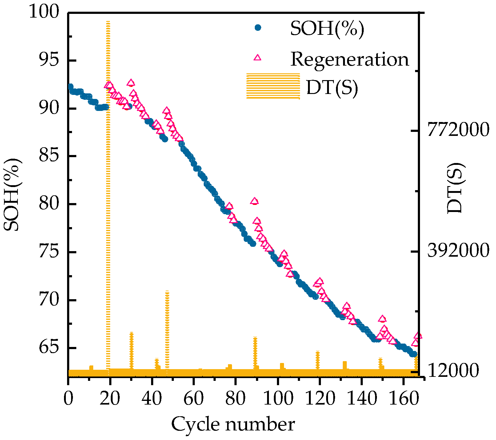
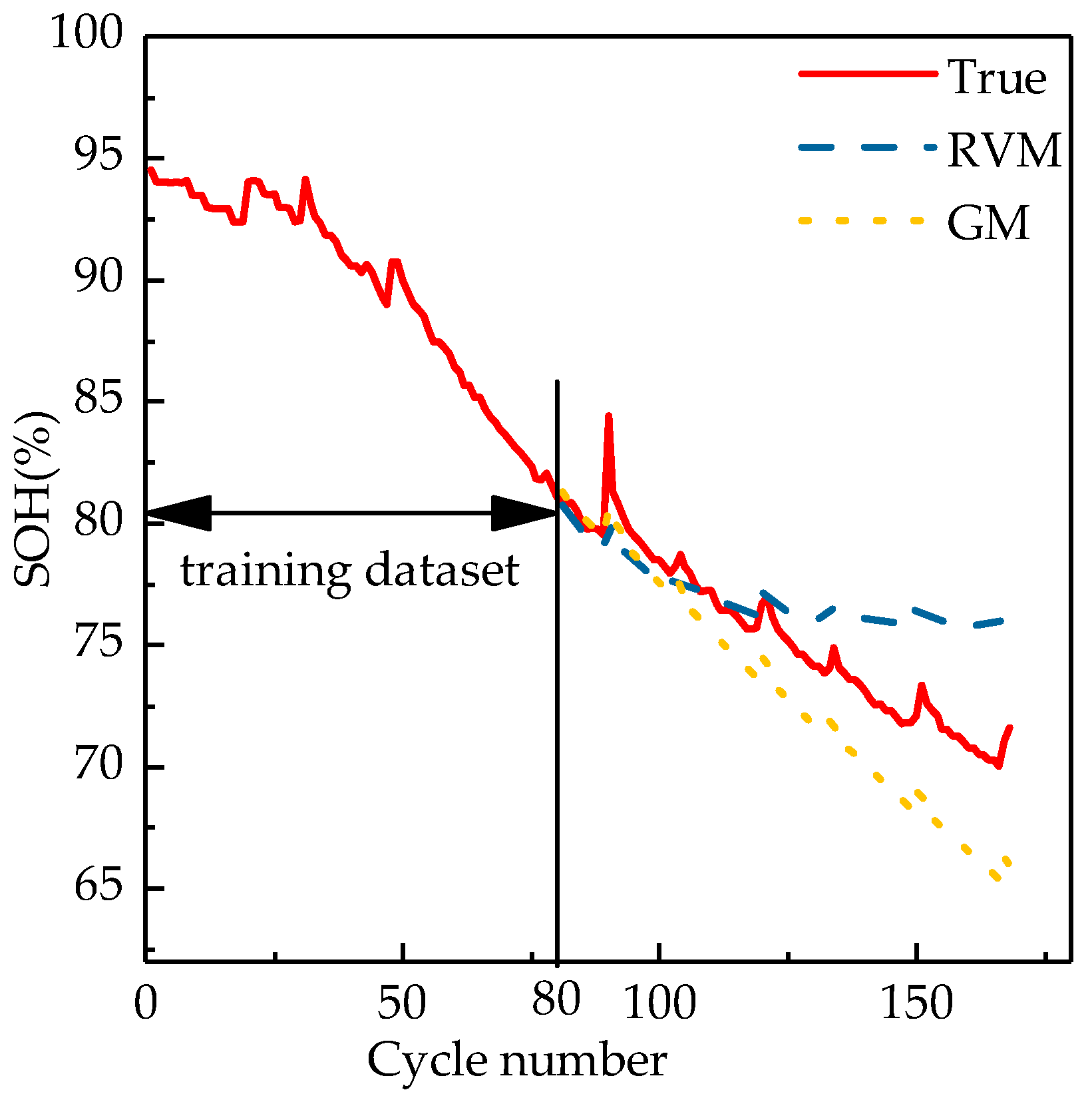
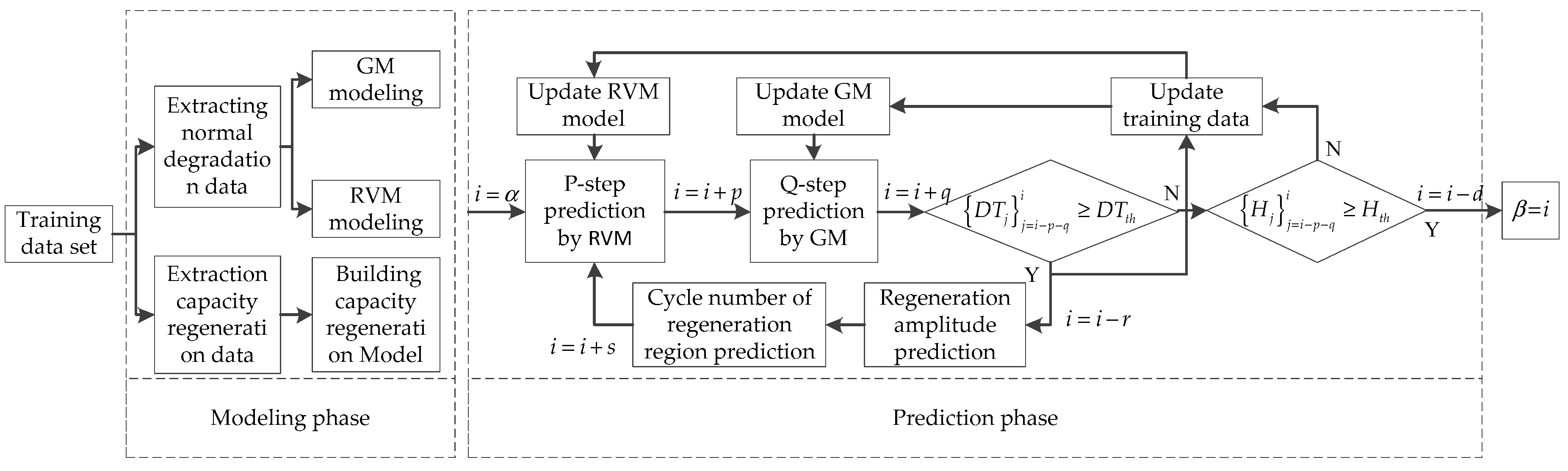
3.1. Lithium-Ion Battery RUL Prognostics

Capacity and internal resistance are the two most commonly used health indicators for lithium-ion battery RUL prognostics. The cost of measuring internal resistance online is too high, but the capacity can be calculated easily by integrating the current over time. In order to represent the SOH of a lithium-ion battery for the RUL prognostics in a unified form, capacity is typically converted as follows:

$$SO{H}_i=\frac{C_i}{C_0}\times 100\%,$$

(21)

where $C_i$ and $C_0$ are the capacity of the cycle $i$ and the rated capacity, respectively. When $C_i$ is less than 70% of $C_0$, the battery reaches the end-of-life.

It is assumed that $\alpha$ is the current charge-discharge cycle and $\beta$ is the cycle at the end-of-life. By predicting the end-of-life cycle number $\beta$, we can get the battery RUL at the $\alpha$ cycle as follows:

$$RU{L}_{\alpha }=\beta -\alpha ,$$

(22)

Figure 1 shows the degradation curve of the #5 lithium-ion battery’s SOH with the cycle number and calendar time. The test data were released by the NASA Prognostics Center of Excellence (PCoE) at the Ames Research Center [33]. In Figure 1, DT indicates the rest time of two adjacent discharge cycles. The red triangle shows the capacity regeneration phenomenon. From Figure 1, the capacity regeneration phenomenon affects the state and rate of degradation. When the rest time is long enough, the battery capacity will be regenerated, and the battery’s SOH will be increased. Moreover, after a visible regeneration appearance, the SOH degradation rate of the next several cycles is much faster than before. Therefore, it is beneficial to take into account the effect of rest time on the prediction which improves the accuracy of the RUL prediction. Similar to some of the concepts Qin et al. [30] defined, in this paper, the cycle with a significant capacity increase caused by a long rest time is called the “regeneration cycle”, the capacity regeneration cycles is called the “regeneration region”, the number of cycles in each regeneration region is called the “regeneration cycle number”, and the cycle except regeneration regions is called the “normal degradation”.

3.2. Hybrid RVM-GM Prediction Method

Our purpose is to get a more accurate battery RUL long-term prediction. Hence, taking into account the effect of the regenerative phenomena, we extract the SOH values of the regeneration cycle, the regeneration cycle number, and normal degradation from the SOH sequence and predict them, respectively.

Figure 2 shows the RVM and GM prediction curves of the #5 battery starting prediction at cycle 80. Starting prediction at cycle 80 means the length of the training data is 80, which is a long-term prediction for the battery’s RUL. Although the RVM and GM can describe future trends of the degradation, the long-term prediction performance is still unsatisfactory. The SOH prediction results of the RVM are accurate over the first few cycles, but the accuracy will lose or even diverge after a few cycles. This problem occurs because the relevance vectors are easily affected by data noise and the coefficients matrix of the trained RVM cannot be updated during the prediction process. The GM identifies the different degree of the development trend among the system factors to predict the trend of the system, but disregards the uncertainty among the factors in the system. To predict the normal degradation trends more accurately, we propose a hybrid model for fusing the RVM and GM. Figure 3 illustrates the framework of the hybrid RVM-GM prediction method. This framework includes the modeling phase and the prediction phase. The execution steps are as follows:

Step 1 decoupling the training data into two parts of normal degradation and regeneration.

Step 2 modeling of the capacity regeneration based on rest time.

Step 3 modeling of the normal degradation by the RVM and the GM.

Step 4 predicting the normal degradation and regeneration region, respectively. In particular, the normal degradation is predicted by the alternating iterative method of the RVM-GM.

Step 5 adding the predicted SOH results of each regeneration region into the normal degradation prediction sequence and getting the final SOH prediction results.

We assume that the battery is fully charged and discharged in each cycle. Thus, we can get the time sequence of the SOH ${\left\{H_k\right\}}_{k=1}^{\alpha }$ and the start time sequence of two adjacent discharge cycles from cycle 1 to cycle $\alpha$, where $\alpha$ is the length of training data.

In the modelling phase, we decouple normal degradation and regeneration from the training data, using $s_k$ to distinguish whether there is a visible SOH regeneration at the $k$th cycle.

$$s_k=\{\begin{array}{l}1, D{H}_k<D{H}_{th}\\ -1, D{H}_k\ge D{H}_{th}\end{array},$$

(23)

where $D{H}_k=H_{k+1}-H_k$ is the forward difference of the SOH between the $k$th and the $\left(k+1\right)$th cycle, $D{H}_{th}$ is the threshold for capacity regeneration. $s_k=1$ means normal degradation, and $s_k=-1$ means that there is a visible SOH regeneration from cycle $k$th to $\left(k+1\right)$th.

The set of cycle indices before a regeneration phenomenon can be represented as $\mathit{A}=\left\{k|{\mathrm{s}}_k=-1,k\in \left\{1,2,\cdots ,\alpha -1\right\}\right\}$. The number of elements in the set $\mathit{A}$ is $N_a$, which indicates the number of regeneration phenomena in the training data. The cycle index of the regeneration region can be extracted according to $\mathit{A}$, which can be represented as $\mathit{B}=\left\{k+j|H_{k+j}>H_k,k\in \mathit{A},j\in N^{+}\right\}$. Continuous cycles in $\mathit{B}$ means a regeneration region. According to the division, the cycles of each regeneration region can be determined. As a result, the cycle index of the normal degenerate can be extracted, which can be represented as $\mathit{E}=\left\{k|k\in \left\{1,2,\cdots ,\alpha \right\},k\notin \mathit{B}\right\}$.

Based on the decoupled data, the RVM and the GM for normal degradation and the rest time-based model for regeneration phenomenon are trained. Moreover, the training data set for the RVM is ${\mathit{R}}_{RVM}=\left\{\left(H_k,H_{k+1}\right)|k,k+1\in \mathit{E}\right\}$, and the original sequences training data set for the GM is ${\mathit{X}}_{GRAY}^{\left(0\right)}=\left\{H_k|k\in \mathit{E}\right\}$.

To predict the regeneration phenomenon, we need to model the regeneration amplitude and the regeneration cycle number, respectively. Figure 4 shows the data points and fitting curves of the rest time and regeneration amplitude of the experimental data of four groups of batteries, indicating a nonlinear relationship. Furthermore, it can be seen that after a visible regeneration, the SOH degradation rate at the next several cycles will be much faster than before. Qin et al. [30] assumed that the growth rate of the regeneration amplitude decreased with an increase in rest time and that the degradation of the capacity regeneration region was a uniform linear process, and therefore the regeneration amplitude and the regeneration cycle number are accurately predicted. However, the modeling of the degradation process in the regeneration region was not accurate. By observing the data of [33], we find that the degradation process of the regeneration zone was decreasing exponentially. Therefore, by obtaining the regeneration amplitude and the regeneration quantity prediction model, the regeneration area is modelled using the exponential model.

The rest time is defined as the forward difference of the beginning time of each cycle, which can be represented as:

$$D{T}_k=T_{k+1}-T_k,$$

(24)

The rest times dataset for estimating regeneration phenomena is

$$D{H}_i^e=s\cdot \varphi \left(D{T}_i^e\right),$$

(25)

$$NU{M}_i^e=\left[\varphi \left(D{T}_i^e\right)\cdot \left(\frac{1}{N_a}{\displaystyle \sum _{j=1}^{N_a}\frac{NU{M}_j}{\varphi \left(D{T}_j^e\right)}}\right)+\frac{1}{2}\right],$$

(26)

where $s$ is a scale parameter, $\varphi (•)$ is a hyperbolic tangent function, $NU{M}_i^e$ is the regeneration cycle number to be estimated, $N_a$ is the number of times that regeneration occurs in the training data, and $NU{M}_j$ is the cycle number of the $j$th regeneration in the training data.

When using the exponential degradation model to model the regeneration region, it is assumed that $j$ is the cycle number before the $i$th regeneration and the health state sequence of the regeneration region can be expressed as follows:

$$R{H}_k^e=H_j+D{H}_i^e-a\cdot \exp \left(b\cdot \left(k-j\right)\right),$$

(27)

where $a$ and $b$ are undetermined parameters.

In the prediction phase, we use the RVM and the GM alternately to carry out a multi-step prediction. We suppose that the plan for future use of the battery is known, which means ${\left\{T_k\right\}}_{k=\alpha +1}^n$ is known.

The rest time sequence ${\left\{D{T}_k^p\right\}}_{k=\alpha +1}^{n-1}$ used for prediction is obtained by Equation (26).

Because the SOH of the prediction process is unknown, we use the rest time threshold $D{T}_{th}$ to indicate the occurrence of regeneration.

The regeneration amplitude set ${\left\{D{H}_k^p\right\}}_{k=1}^M$, and the regeneration quantity set ${\left\{NU{M}_k^p\right\}}_{k=1}^M$ is predicted by Equations (25) and (26), where $M$ is the number of times that regeneration occurs in the prediction process. Our proposed hybrid prediction algorithm is summarized as Algorithm 1.

Algorithm 1

● Input: train dataset ${\mathit{R}}_{RVM}$ and ${\mathit{X}}_{gray}^{\left(0\right)}$, RVM model, regeneration amplitude dataset ${\left\{D{H}_k^p\right\}}_{k=1}^M$, regeneration number dataset ${\left\{NU{M}_k^p\right\}}_{k=1}^M$, SOH threshold $H_{th}$ 1. while $i<n-1$ 2. if $H_{i-1}^p>H_{th}$ and $H_{i-2}^p<H_{th}$ 3. set ${\beta }^p=i-1$ 4. end 5. if the $s$ cycle regeneration and $s\in [i-p-q,i-1]$ 6. set $i=s+1$ 7. set $H_j^p=H_s^p$ 8. for $k=1 to NU{M}_j^p$ 9. set $H_i^p=H_j^p+D{H}_j^p-a\cdot \exp \left(b\cdot k\right)$ 10. set $i=i+1$ 11. end 12. set $j=j+1$ 13. Remove $H_{i-NU{M}_j^p}^p$ to $H_i^p$ from dataset ${\mathit{X}}_{gray}^{\left(0\right)}$ 14. else 15. for $k=1 to p$ 16. set $H_{i-1}^p$ as the input of the RVM model 17. predict $H_i^p$ by RVM model 18. put $H_i^p$ into the dataset ${\mathit{X}}_{gray}^{\left(0\right)}$ 19. set $i=i+1$ 20. end 21. predict $H_i^p$ to $H_{i+q}^p$ by GRAY model 22. put $H_i^p$ to $H_{i+q}^p$ in to set ${\mathit{X}}_{gray}^{\left(0\right)}$ 23. set $i=i+q$ 24. set new dataset ${\mathit{R}}_{RVM}^{new}=\left\{{\mathit{R}}_{RVM},\left(H_{i-1}^p,H_i^p\right)\right\}$ 25. retrain the RVM model by new ${\mathit{R}}_{RVM}^{new}$ 26. set $i=i+1$ 27. end 28. end ● output: end life cycle number ${\beta }^p$, SOH prediction results ${\left\{H_k^p\right\}}_{k=\alpha +1}^n$

During the prediction process, all the new prediction results are added to the original sequence to update the GM. However, in contrast to the iterative updating strategy proposed by [15], which adds all the prediction results to the training dataset of the RVM, all we need is the original dataset and the latest prediction results. Because the GM cannot carry out an accurate local prediction, adding all the GM prediction results in the training set of the RVM will reduce the prediction accuracy.

4. Results and Discussion

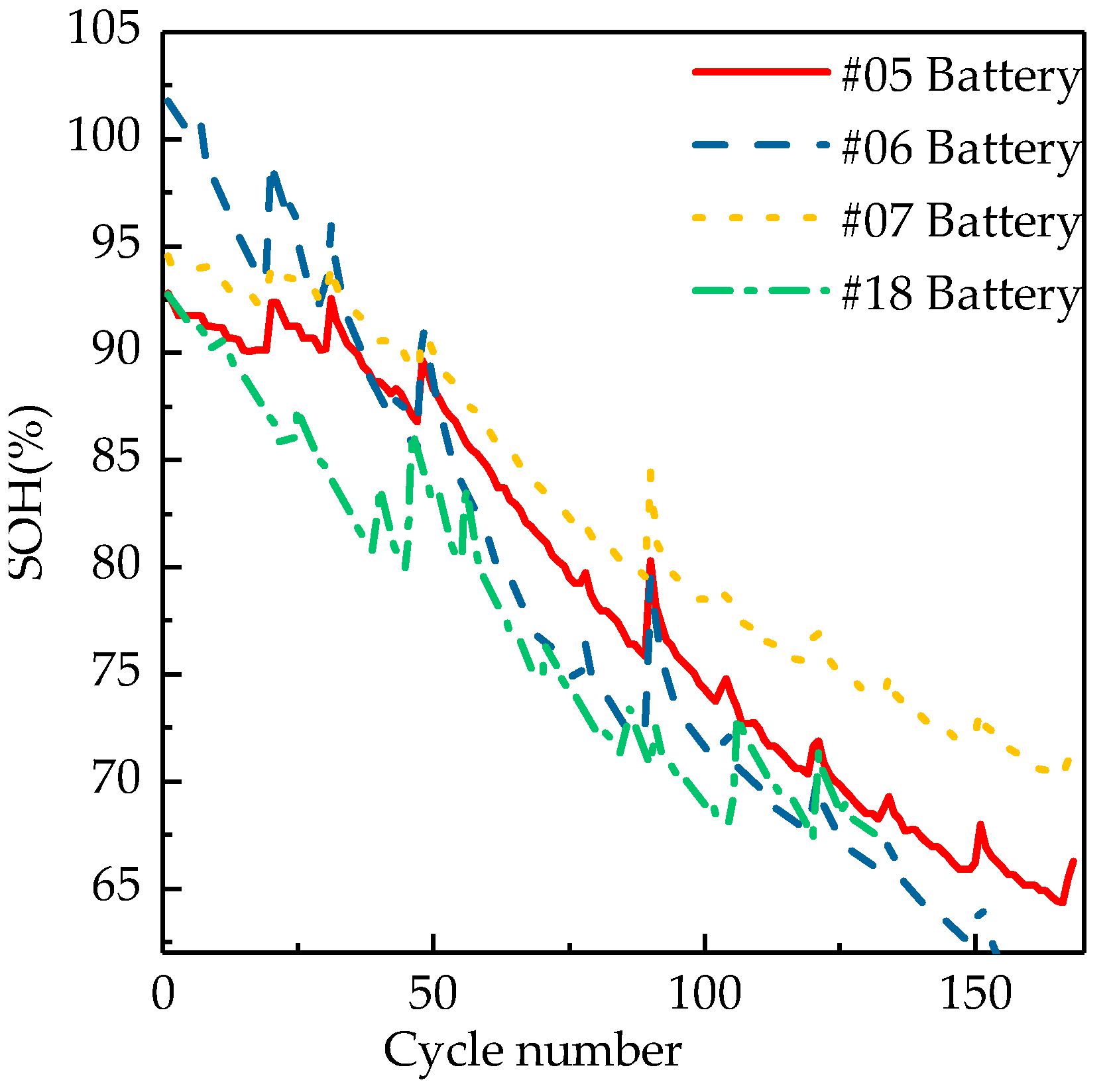
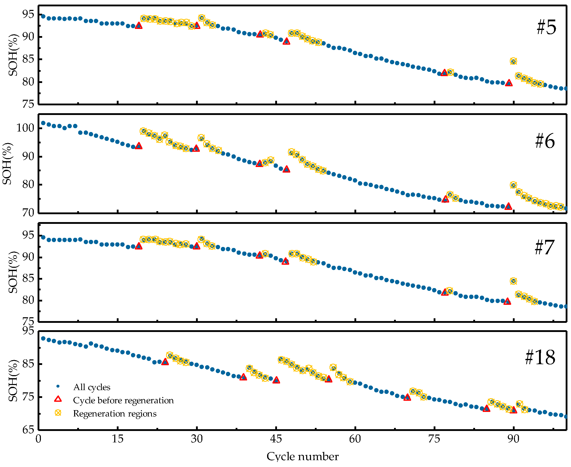
4.1. Experiment Battery Dataset

The effectiveness of our proposed method is verified by the lithium-ion battery experimental data provided by the NASA PCoE [33]. This experimental dataset which consisted of 18,650 commercial lithium-ion battery sets was obtained by charging and discharging in cycles at room temperature. Details of the experiment can be found in reference [33]. We used the experimental data of batteries #5, #6, #7, and #18. The batteries reached the end-of-life when their capacity was reduced to 30% of the rated capacity.

Figure 5 shows the SOH degradation curves of batteries #5, #6, #7, and #18. We can see that each battery has some visible SOH regeneration, and the SOH degradation rate at the next several cycles of regeneration will be much faster than before. In our experiment, the initial capacity value is set to 2 Ah and the end-of-life capacity is set to 1.4 Ah. The battery data length for batteries #5, #6, and #7 is 168, and #18 is 132. The actual life cycle of batteries #5, #6, and #18 is 124, 109, and 121, respectively. For battery #7, the capacity decreases to 1.432 Ah at the end. When we set its end-of-life capacity threshold at 72%, then its actual life cycle is 146.

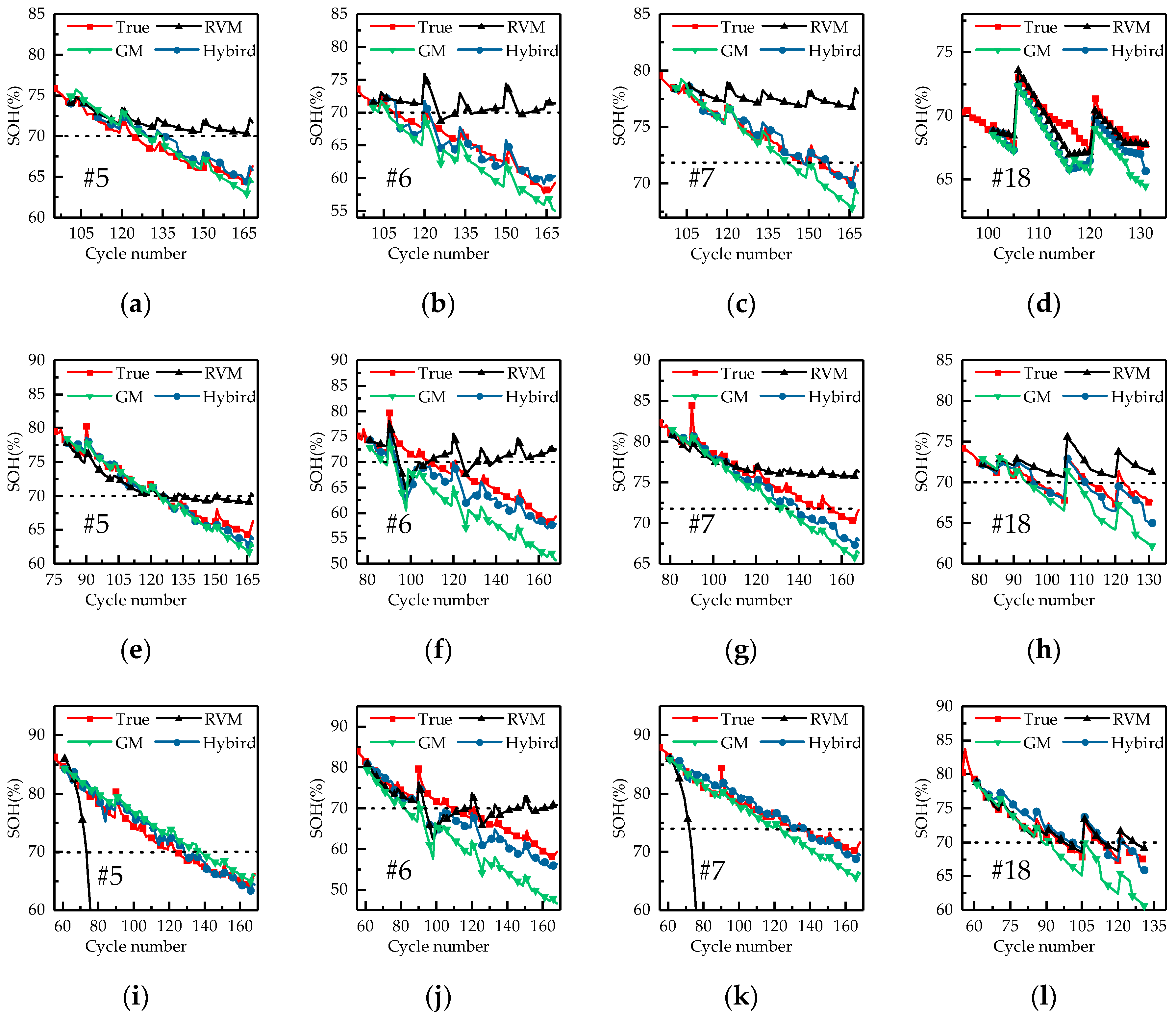
4.2. Experiment and Discussion

Figure 6 shows the results of normal degradation and capacity regeneration decoupling of the first 100 cycle data of each battery. We can see that the starting time of the capacity regeneration in batteries #5, #6, and #7 is the same, because the starting time of each charge-discharge cycle is the same during the three battery tests. However, due to the influence of initial conditions and other uncertainties in the test process, the regeneration amplitude and quantity of those three batteries are different.

The absolute error of the RUL prediction results and the root mean square error of the SOH prediction results are used to quantify and evaluate the prediction results, which are defined as follows:

$$AE=\left|\beta -{\beta }^p\right|,$$

(28)

$$RMSE=\sqrt{\frac{1}{n-\alpha }{\displaystyle \sum _{i=\alpha +1}^n{\left(H_i-H_i^p\right)}^2}},$$

(29)

The prediction comparison for the RVM, the GM, and the hybrid method for batteries #5, #6, #7, and #18 are shown in

Table 1. Comparison of prediction results of the hybrid method with the relevance vector machine (RVM) and the gray model (GM).

Prediction Start Cycle	Battery Number	Hybrid Model		RVM		GM
		AE	RMSE (%)	AE	RMSE (%)	AE	RMSE (%)
100	#5	4	0.960422	-	3.59411	4	1.025602
	#6	1	1.241741	16	6.886879	2	2.576045
	#7	1	0.921971	-	4.071211	5	1.099363
	#18	-	1.520362	-	0.803822	-	1.95701
80	#5	1	0.8253	1	2.27695	1	1.132771
	#6	15	3.06826	14	6.679174	16	6.349727
	#7	7	1.191789	-	2.726045	16	2.48364
	#18	1	1.015091	-	2.278513	3	2.664143
60	#5	4	1.033175	54	69.82189	13	2.724726
	#6	15	3.338834	15	5.403552	26	8.576316
	#7	1	0.996845	74	69.76426	12	2.203527
	#18	4	1.111508	1	0.708308	8	3.333486

and Figure 7. The prediction start cycle means predicting the RUL at the current cycle, and the length of the training data is equal to the started prediction cycle. It can be seen from Table 1 that the RUL prediction errors of our hybrid are less than the single RVM and the single GM method at a different started predicton cycle. Moreover, the AE and RMSE are also smaller than the single model. The error message illustrates that our method has high accuracy over the prediction period. The performance of the hybrid model is still satisfied with the expansion of the prediction horizon. More specifically, the prognostic AE started prediction at cycle 60 of batteries #5, #6, #7, and #18 among the single RVM methods 54, 15, 74, and 1, respectively. But, the counterparts of our hybrid model are 4, 15, 1, and 4, respectively. Although the AE on battery #18 is slightly larger, we can see that the prognostic of the proposed method is more accurate and stable. Similarly, as compared with the single GM method, the prognostic results on four batteries are the smallest.

To compare more broadly with other types of prediction methods, we investigated many other model-based and data-driven approaches. The RVM-KF method proposed in references [15] is based on the empirical model, RVM and Kalman filter for lithium-ion battery prognostic without considering the influence of the regeneration phenomenon, although they did not give the experimental results of battery #18, which was heavily affected by the regeneration phenomenon. The proposed hybrid method not only accurately predicts the local regeneration phenomenon but also has higher accuracy in predicting the battery RUL for short-term and long-term.

Table 2. Comparison of prediction results of the hybrid RVM-GM method with RVM-KF.

Battery Number	Prediction Start Cycle	Absolute Error of RUL Prediction Result
		Hybrid Method	RVM-KF Method
#5	60	28	4
	80	8	1
	100	4	4
#6	60	32	15
	80	2	15
	90	3	2
#7	60	39	1
	80	19	7
	100	1	1
#18	60	4	8
	80	1	5
	100	-	-

shows the comparison of prediction results of the hybrid method with the RVM-KF method. It should be noted that the RVM-KF algorithm has better prediction performance than the proposed hybrid method started prediction at cycle 80 of battery #6. One possible reason is that the hybird method does not accurately predict the abnormal regeneration, and the end-of-life is in this inaccurate prediction. The rest time-based prognostic method proposed in reference [30] uses the data-driven method of the SVM and the Gaussian process model for lithium-ion battery prognostic.However, they only gave short-term prediction results for started prediction at the start cycle 100. The present experiment is started at different stages of battery life, and the prediction performance is better in both the short- and long-term prognostic. Moreover, as compared with the electrochemical model [2] and the equivalent circuit model [8,25,34] methods that provide high-precision short-term SOH prediction, the proposed hybrid method not only provides very closed short-term SOH prediction accuracy, but also provides effective long-term RUL prediction results.

5. Conclusions

To improve the long-term RUL prediction performance of the lithium-ion battery with capacity regeneration phenomenon, a hybrid prediction method based on the RVM and the GM algorithm is explored. The proposed method decouples regeneration phenomenon and normal degradation and predicts them separately. After obtaining the amplitude of regeneration and the regeneration cycle number, an exponential model is proposed to describe the degraded region. Moreover, an iterative updating method is proposed to predict the normal degradation. The RVM and the GM are alternately used to carry out a multi-step prediction. The RVM-GM model prediction results update the training dataset, and the updated training dataset retrains the RVM-GM model. Finally, we add the prediction results of each regeneration region into the normal degradation prediction sequence to get the overall SOH prediction results.

As compared with a pure RVM and a pure GM, our hybrid method has higher accuracy and stability. Moreover, the RVM and the GM in the proposed hybrid method only rely on historical data, and it can construct a prognostic model without any prior knowledge about the complex battery degradation. Thereby, this method can predict the RUL of different types of batteries with historical data accumulation.

The limitations of our hybrid method in real applications are that the training data should have typical data reflecting the regenerated phenomena, and the future battery use plan should be known to determine the rest time in the prediction phase. In addition, other factors such as temperature and hysteresis can also affect the accuracy of the prediction. Therefore, our future work will investigate how to build the degradation model in the case of insufficient data and will consider the influence of unknown rest time, temperature, data lag, and other factors on the prediction uncertainty.

References

1. Su, C.; Chen, H.J. A review on prognostics approaches for remaining useful life of lithium-ion battery. In International Conference on New Energy and Future Energy System, Kunming, China, 22–25 September 2017; Kyriakopoulos, G.L., Ed.; IOP Publishing: Bristol, UK, 2017; Volume 93, p. 012040. [Google Scholar] [Green Version]
2. Lyu, C.; Lai, Q.; Ge, T.; Yu, H.; Wang, L.; Ma, N. A lead-acid battery’s remaining useful life prediction by using electrochemical model in the particle filtering framework. Energy 2017, 120, 975–984. [Google Scholar] [CrossRef]
3. Barre, A.; Deguilhem, B.; Grolleau, S.; Gerard, M.; Suard, F.; Riu, D. A review on lithium-ion battery ageing mechanisms and estimations for automotive applications. J. Power Sources 2013, 241, 680–689. [Google Scholar] [CrossRef]
4. Liu, D.; Yin, X.; Song, Y.; Liu, W.; Peng, Y. An on-line state of health estimation of lithium-ion battery using unscented particle filter. Ieee Access 2018, 6, 40990–41001. [Google Scholar] [CrossRef]
5. Omariba, Z.B.; Zhang, L.; Sun, D. Review on health management system for lithium-ion batteries of electric vehicles. Electronics 2018, 7, 72. [Google Scholar] [CrossRef]
6. Li, F.; Xu, J. A new prognostics method for state of health estimation of lithium-ion batteries based on a mixture of gaussian process models and particle filter. Microelectron. Reliab. 2015, 55, 1035–1045. [Google Scholar] [CrossRef]
7. Chang, Y.; Fang, H.; Zhang, Y. A new hybrid method for the prediction of the remaining useful life of a lithium-ion battery. Appl. Energy 2017, 206, 1564–1578. [Google Scholar] [CrossRef]
8. Hu, X.; Li, S.; Peng, H. A comparative study of equivalent circuit models for li-ion batteries. J. Power Sources 2012, 198, 359–367. [Google Scholar] [CrossRef]
9. Zhang, L.; Mu, Z.; Sun, C. Remaining useful life prediction for lithium-ion batteries based on exponential model and particle filter. IEEE Access 2018, 6, 17729–17740. [Google Scholar] [CrossRef]
10. Su, X.; Wang, S.; Pecht, M.; Ma, P.; Zhao, L. Prognostics of lithium-ion batteries based on different dimensional state equations in the particle filtering method. Trans. Inst. Meas. Control 2017, 39, 1537–1546. [Google Scholar] [CrossRef]
11. Yang, F.; Wang, D.; Xing, Y.; Tsui, K.-L. Prognostics of li(nimnco)o-2-based lithium-ion batteries using a novel battery degradation model. Microelectron. Reliab. 2017, 70, 70–78. [Google Scholar] [CrossRef]
12. Wang, D.; Miao, Q.; Pecht, M. Prognostics of lithium-ion batteries based on relevance vectors and a conditional three-parameter capacity degradation model. J. Power Sources 2013, 239, 253–264. [Google Scholar] [CrossRef]
13. Saha, B.; Goebel, K.; Poll, S.; Christophersen, J. Prognostics methods for battery health monitoring using a bayesian framework. IEEE Trans. Instrum. Meas. 2009, 58, 291–296. [Google Scholar] [CrossRef]
14. Xing, Y.J.; Ma, E.W.M.; Tsui, K.L.; Pecht, M. An ensemble model for predicting the remaining useful performance of lithium-ion batteries. Microelectron. Reliab. 2013, 53, 811–820. [Google Scholar] [CrossRef]
15. Song, Y.; Liu, D.; Hou, Y.; Yu, J.; Peng, Y. Satellite lithium-ion battery remaining useful life estimation with an iterative updated rvm fused with the kf algorithm. Chin. J. Aeronaut. 2018, 31, 31–40. [Google Scholar] [CrossRef]
16. Zheng, X.; Fang, H. An integrated unscented kalman filter and relevance vector regression approach for lithium-ion battery remaining useful life and short-term capacity prediction. Reliab. Eng. Syst. Saf. 2015, 144, 74–82. [Google Scholar] [CrossRef]
17. Wei, J.; Dong, G.; Chen, Z. Remaining useful life prediction and state of health diagnosis for lithium-ion batteries using particle filter and support vector regression. IEEE Trans. Ind. Electron. 2018, 65, 5634–5643. [Google Scholar] [CrossRef]
18. Wu, L.; Fu, X.; Guan, Y. Review of the remaining useful life prognostics of vehicle lithium-ion batteries using data-driven methodologies. Appl. Sci. 2016, 6, 166. [Google Scholar] [CrossRef]
19. Zhang, Y.; Xiong, R.; He, H.; Pecht, M.G. Long short-term memory recurrent neural network for remaining useful life prediction of lithium-ion batteries. IEEE Trans. Veh. Technol. 2018, 67, 5695–5705. [Google Scholar] [CrossRef]
20. Sbarufatti, C.; Corbetta, M.; Giglio, M.; Cadini, F. Adaptive prognosis of lithium-ion batteries based on the combination of particle filters and radial basis function neural networks. J. Power Sources 2017, 344, 128–140. [Google Scholar] [CrossRef]
21. Gao, D.; Huang, M. Prediction of remaining useful life of lithium-ion battery based on multi-kernel support vector machine with particle swarm optimization. J. Power Electron. 2017, 17, 1288–1297. [Google Scholar]
22. Zhao, Q.; Qin, X.; Zhao, H.; Feng, W. A novel prediction method based on the support vector regression for the remaining useful life of lithium-ion batteries. Microelectron. Reliab. 2018, 85, 99–108. [Google Scholar] [CrossRef]
23. Yang, W.-A.; Xiao, M.; Zhou, W.; Guo, Y.; Liao, W. A hybrid prognostic approach for remaining useful life prediction of lithium-ion batteries. Shock and Vibration 2016, 2016, 3838765. [Google Scholar] [CrossRef]
24. Liao, L.; Koettig, F. A hybrid framework combining data-driven and model-based methods for system remaining useful life prediction. Appl. Soft Comput. 2016, 44, 191–199. [Google Scholar] [CrossRef]
25. Liu, J.; Wang, W.; Ma, F.; Yang, Y.B.; Yang, C.S. A data-model-fusion prognostic framework for dynamic system state forecasting. Eng. Appl. Artif. Intell. 2012, 25, 814–823. [Google Scholar] [CrossRef] [Green Version]
26. Dong, G.; Chen, Z.; Wei, J.; Ling, Q. Battery health prognosis using brownian motion modeling and particle filtering. IEEE Trans. Ind. Electron. 2018, 65, 8646–8655. [Google Scholar] [CrossRef]
27. Zhou, Y.; Huang, M. Lithium-ion batteries remaining useful life prediction based on a mixture of empirical mode decomposition and arima model. Microelectron. Reliab. 2016, 65, 265–273. [Google Scholar] [CrossRef]
28. Zhang, J.; He, X.; Si, X.; Hu, C.; Zhou, D. A novel multi-phase stochastic model for lithium-ion batteries’ degradation with regeneration phenomena. Energies 2017, 10, 1687. [Google Scholar] [CrossRef]
29. Liu, D.; Zhou, J.; Liao, H.; Peng, Y.; Peng, X. A health indicator extraction and optimization framework for lithium-ion battery degradation modeling and prognostics. IEEE Trans. Syst. Man Cybern.-Syst. 2015, 45, 915–928. [Google Scholar]
30. Qin, T.; Zeng, S.; Guo, J.; Skaf, Z. A rest time-based prognostic framework for state of health estimation of lithium-ion batteries with regeneration phenomena. Energies 2016, 9, 896. [Google Scholar] [CrossRef]
31. Tipping, M.E. Sparse bayesian learning and the relevance vector machine. J. Mach. Learn. Res. 2001, 1, 211–244. [Google Scholar]
32. Zhou, Z.; Huang, Y.; Lu, Y.; Shi, Z.; Zhu, L.; Wu, J.; Li, H. Lithium-ion battery remaining useful life prediction under grey theory framework. In Proceedings of the 2014 prognostics and system health management conference, Zhangjiajie, China, 24–27 August 2014; IEEE: Piscataway, NJ, USA; pp. 297–300. [Google Scholar]
33. Goebel, B.S.a.K. Battery data set. National Aeronautics and Space Adminstration (NASA) Ames Prognostics Data Repository.; Moffett Field: CA, USA, 2007. Available online: https://ti.arc.nasa.gov/tech/dash/groups/pcoe/prognostic-data-repository/ (accessed on 20 October 2018).
34. Eddahech, A.; Briat, O.; Vinassa, J.-M. Lithium-ion battery performance improvement based on capacity recovery exploitation. Electrochim. Acta 2013, 114, 750–757. [Google Scholar] [CrossRef]
Figure 1. Degradation curve of the state of health (SOH) with cycle number and calendar time for #5 battery.
Applsci 09 01890 g001
Figure 2. Relevance vector machine (RVM) and gray model (GM) prediction curve starting prediction at the cycle 80 of the #5 battery.
Applsci 09 01890 g002
Figure 3. The framework of the hybrid RVM and GM model (RVM-GM) prediction method.
Applsci 09 01890 g003
Figure 4. The relationship between rest time and the amplitude of the SOH regeneration.
Applsci 09 01890 g004
Figure 5. The SOH degradation with the cycle of batteries #5, #6, #7, and #18.
Applsci 09 01890 g005
Figure 6. The extraction of normal degradation and capacity regeneration.
Applsci 09 01890 g006
Figure 7. Prediction results at different started prediction cycles of different batteries. (a) Started prediction at cycle 100 of battery #5, (b) Started prediction at cycle 100 of battery #6, (c) Started prediction at cycle 100 of battery #7, (d) Started prediction at cycle 100 of battery #18, (e) Started prediction at cycle 80 of battery #5, (f) Started prediction at cycle 80 of battery #6, (g) Started prediction at cycle 80 of battery #7, (h) Started prediction at cycle 80 of battery #18, (i) Started prediction at cycle 60 of battery #5, (j) Started prediction at cycle 60 of battery #6, (k) Started prediction at cycle 60 of battery #7, (l) Started prediction at cycle 60 of battery #18.
Applsci 09 01890 g007