A Deep Learning Method for Bearing Fault Diagnosis through Stacked Residual Dilated Convolutions


School of Mechanical Engineering, Shanghai Jiao Tong University, Shanghai 200240, China
*
Author to whom correspondence should be addressed.
Appl. Sci. 2019, 9(9), 1823; https://doi.org/10.3390/app9091823
Submission received: 25 March 2019
/
Revised: 24 April 2019
/
Accepted: 30 April 2019
/
Published: 1 May 2019
(This article belongs to the Special Issue Advances in Deep Learning)
Abstract
:Real-time monitoring and fault diagnosis of bearings are of great significance to improve production safety, prevent major accidents, and reduce production costs. However, there are three primary concerns in the current research, namely real-time performance, effectiveness, and generalization performance. In this paper, a deep learning method based on stacked residual dilated convolutional neural network (SRDCNN) is proposed for real-time bearing fault diagnosis, which is subtly combined by the dilated convolution, the input gate structure of long short-term memory network (LSTM) and the residual network. In the SRDCNN model, the dilated convolution is used to exponentially increase the receptive field of convolution kernel and extract features from the sample with more points, alleviating the influence of randomness. The input gate structure of LSTM could effectively remove noise and control the entry of information contained in the input sample. Meanwhile, the residual network is introduced to overcome the problem of vanishing gradients caused by the deeper structure of the neural network, hence improving the overall classification accuracy. The experimental results indicate that compared with three excellent models, the proposed SRDCNN model has higher denoising ability and better workload adaptability.
1. Introduction
With the rapid development of manufacturing technology and the increasing complexity of manufacturing systems, the challenges of safety and reliability requirements for manufacturing equipment and mechanical products have become extremely important. Their failure will not only lead to production interruptions, but also increase the operating costs of the company.
Rolling element bearing (REB) is one of the key components of industrial transmission systems and plays an extremely important role in supporting and transmitting power. Although bearings have already been widely used in aerospace, vehicles, ships, and other important fields, they are one of the vulnerable parts of rotating machinery in terms of the current manufacturing technology and actual working conditions. Research shows that an approximately 30% of failures in rotating machinery are caused by bearing damage. Therefore, it remains a challenge to ensure production safety, as well as to reduce production costs by monitoring and diagnosing the bearing state [1]. In the last two decades, bearing fault diagnosis has already attracted extensive attention [2]. Many monitoring techniques have been applied to the monitoring and diagnosis of bearings [3]. The most common solution is to analyze the bearing signals continuously collected by the vibration monitoring system installed on the rotating machines and provide real-time monitoring and warning [4].
The goal of bearing fault diagnosis is to establish an effective real-time condition monitoring and identification system to ensure continuous production through predictive maintenance. In order to achieve this goal, there are three main challenges to address:
- To meet the requirements of real-time fault diagnosis of rotating machinery, the fault diagnosis model needs to perform continuous and rapid diagnosis based on the vibration signal collected in real-time [5].
- To improve the effectiveness of the fault diagnosis model, the essential features need to be extracted to avoid local false features caused by ambient noise and fluctuations in working conditions [6].
- To keep good performance under different working conditions, the fault diagnosis model needs to have good generalization performance under different load and noise conditions [7].
Various methods have been developed for the fault diagnosis of bearings. Zhang and Randall [8] designed the parameters for optimal resonance demodulation, using the fast kurtogram for initial estimates and the genetic algorithm for final optimization. Wang et al. [9] combined the merits of ensemble local mean decomposition and fast kurtogram to detect the fault for rotating machinery. Nevertheless, traditional feature extraction methods require a great deal of domain expertise and prior knowledge, which limits the mining of new features.
Previous studies have shown that the accuracy of classifying results is largely dependent on the extracted features. To automatically learn feature representations from raw data, Hinton et al. [10] drew on the hierarchical learning process of human brain and proposed a milestone deep learning model training paradigm. Deep learning has made breakthroughs in natural language processing [11], speech recognition [12], image recognition [13], and other fields. There have been some attempts on feeding the frequency data of vibration signals into deep learning model. Lu et al. [14] carried out a detailed study of stacked denoising autoencoders for bearing fault diagnosis. Zhang et al. [15] presented a deep convolutional neural network with wide first-layer kernels, using the normalized 1025 Fourier coefficients transformed from the raw temporal signals as the input. Jing et al. [16] developed a convolutional neural network (CNN) to learn features from raw data, frequency spectrum and combined time-frequency data, and demonstrated that feature learning with CNN could provide much better results than manual feature extraction.
Considering that deep learning models can directly work on the raw data without any data preprocessing, there have been some deep learning-based bearing fault diagnosis studies working directly on the raw vibration signal to improve the real-time performance of fault diagnosis. Zhang et al. [17] established a one-dimensional deep convolutional neural network (1d-DCNN), which adopted an end-to-end learning method and achieved satisfactory accuracy under a noisy environment. Zhuang and Qin [18] broaden and deepen the neural network and designed an end-to-end one-dimensional multi-scale deep convolutional neural network with few training parameters and a smooth training process. Lu et al. [19] presented a two-dimensional deep convolutional neural network (2d-DCNN) by mapping the raw monitoring signal to feature maps. Wen et al. [20] developed an effective data preprocessing method to convert the time-domain raw signals into images, and built a new CNN based on LeNet-5 to make full use of the experience related to CNN from image processing. Although there has been no agreement on the source of the generalization ability of deep learning, it is no denying that the deep learning method has better generalization performance than most machine learning methods [21,22]. A large number of generalization experiments have been carried out, and the results show that the deep learning model has better generalization performance than the traditional machine learning algorithm [7,14,15,17,19]. From the previous literature, it can be concluded that the deep learning model has almost replaced the traditional feature extraction method and become the popular algorithm for bearing fault diagnosis.
Although the fault diagnosis model based on deep learning can achieve satisfactory real-time and generalization performance, the model is prone to fall into the trap of local false features during the training process, which are greatly affected by the sample quality [23]. The sample quality can be improved to some extent by increasing the redundancy of the sample information by using more points in a sample [14], but the effects of random factors (such as ambient noise and working conditions fluctuation) can’t be fundamentally eliminated. As the redundancy of sample information increases, the model will have a higher potential to resist random factors and avoid local false features. Besides, the detection device in reality has a higher sampling frequency to grasp more operating information and, therefore, the number of sampling points collected per revolution of the machine is increased. In conclusion, it is no longer satisfactory to take just 200–400 data points as one sample of the bearing fault diagnosis model. The number of input layer neurons in the fault diagnosis model needs to be expanded to avoid local false features and to adapt to high frequency dynamic detection.
In order to address the problems above, in this paper, an intelligent fault diagnosis method based on stacked residual dilated convolutional neural network (SRDCNN) is proposed. The main novelties and contributions of this paper are summarized below:
- A novel effective deep learning framework is proposed, which subtly integrates the dilated convolution, the input gate structure of LSTM and the residual network.
- This algorithm performs pretty well under the noisy environment by effectively enlarging the receptive field and controlling the entry of information.
- This algorithm keeps high diagnostic accuracy across different workloads due to the ability to automatically and efficiently extract essential features.
The remainder of the paper is organized as follows: Section 2 presents the overall framework and detailed structure of the SRDCNN-based intelligent fault diagnosis method; in Section 3, some comparative experiments are conducted to evaluate the effectiveness of the proposed intelligent fault diagnosis method against other methods; and Section 4 draws some conclusions and presents the future work.
2. SRDCNN-Based Intelligent Fault Diagnosis Method
Taking the above-mentioned problems into consideration, deep learning method is a promising tool to achieve real-time bearing fault diagnosis. Deep learning methods can learn a stable hierarchical feature representation from the raw bearing vibration signal in an off-line manner, and then diagnose the bearing status online according to the real-time collected vibration signal. Although deep learning has a high potential to avoid false features caused by ambient noise and fluctuations in working conditions, but it still requires ingenious structural design to avoid false features of bearing vibration signals; and thereby improve the performance of bearing fault diagnosis. Han et al. [26] designed an enhanced convolutional neural network with enlarged receptive fields to capture the fault information in the vibration signal. Pan et al. [27] combined one-dimensional CNN and LSTM into one unified structure (LSTM-CNN) to make full use of the classification capabilities of CNN and the time coherence representation ability of LSTM. In this paper, a novel stacked residual dilated convolutional neural network based intelligent fault diagnosis method is proposed for bearing fault diagnosis. In the proposed SRDCNN model, the dilated convolution is employed to exponentially increase the receptive field of convolution kernel and extract essential features from the sample with more points, alleviating the influence of randomness. The input gate structure of LSTM is adopted to effectively remove noise and control the entry of information contained in the input sample. Meanwhile, the residual network is introduced to overcome the problem of vanishing gradients caused by deeper structure of the neural network, hence improving the overall classification accuracy.
2.1. Framework of SRDCNN Model
The overall framework of proposed SRDCNN model is shown in Figure 1. The structure of the SRDCNN model is composed of several residual dilated convolutional layers, the flatten layer and the Softmax layer. Residual dilated convolutional layer is a combination of the dilated convolution, the input gate structure of LSTM and a residual network, which is shown in the partial enlarged detail. For one sample, the length is reduced by half after getting through a residual dilated convolutional layer, which is the most important part of the network structure and will be explained in the next section. In order to adequately mine sample features, multiple filters are used at each residual dilated convolution layer. The flatten layer flattens a plurality of vectors and then flattens them into a one-dimensional vector. The last layer is a dense layer that uses the Softmax function to implement a multi-classification task. The value of each neuron in the output layer indicates the probability that the input sample belongs to a fault category. And the category of the input signal is the one with the highest probability in the output layer of the model.
The input of the SRDCNN model is a sample taken from the bearing vibration signals using a sliding window. To ensure real-time performance, when a new sampling point is collected, the previous sample will discard its first sampling point and add a new sampling point at the end to form a new next sample. After the sample is input into the network, the neurons in each layer are all represented by solid spots. When a new sampling point is collected and used as the end point of the next sample, the outputs of every layer are represented by virtual spots and the dashed line represents the calculation process of the next sample. The points of the same color in Figure 1 are neurons of the same layer.
2.2. Residual Dilated Convolutional Layer
2.2.1. Dilated Convolution
The dilated convolution (also known as convolution with holes) was first proposed by Yu and Koltun [28] to widely reference to multi-scale contextual information without losing resolution. However, it is difficult to design dilated convolution structure for specific application objects. In recent years, dilated convolution has been applied to solve problems such as semantic segmentation [29], speech synthesis [30], and machine translation [31], etc. Borovykh et al. [32] proposed a conditional time series forecasting method based on the dilated convolution, the prediction model can be expressed as: P(y|x1,x2,x3,…,xn). They held that time series data follows a certain probability distribution that could be learned by training. The y predicted was the next value xn+1 of the time series. From another point of view, the probability that the data belongs to a certain class can also be determined according to the distribution law of the time series data. Since the bearing vibration signal is a typical time series data, it is a promising method to determine the state of the bearing by using a dilated convolution, and to obtain the probability distribution of the bearing vibration signal.
As shown in Figure 2, the dilated convolution filter skips input values with a certain step. A dilated convolution is equivalent to a convolution with a larger filter, obtained by filling the original filter with zeros. However, the former is significantly more efficient, and the latter may consume unnecessary costs of training time and storage space. A dilated convolution increases the receptive field without losing information, and the output of each convolution layer contains a wide range of information from input data, which has a great effect on avoiding local false features. For the vibration signal, if the length of a sample is short, the accuracy of the diagnosis model will be greatly affected by the local false features. An effective way is to adopt dilated convolution to accept a longer sample with a large amount of redundant information.
2.2.2. Input Gate Structure of LSTM
Under the framework of the dilated convolution, the network could receive longer input sample to obtain more information. However, the working environment of the bearing is complicated, and the vibration signal often encounters serious noise interference or fluctuations during operation. Even if the input samples of the model contain a lot of information, these factors may make the information untraceable. Therefore, it is necessary to denoise the bearing signal by designing an effective filter. The input gate structure of LSTM [33] can effectively control the input of information from the input samples. Therefore, the input gate structure of LSTM can be regarded as a filter to remove noise. As shown in Figure 3, the input gate has two parts: the sigmoid part it decides which values to update; and the tanh part creates a new candidate vector Ĉt.
2.2.3. Residual Network
As described above, stacked dilated convolution can exponentially expand the receptive field of the network to avoid local false features. However, the depth of network is considerable when the receptive field is quite large. In order to address the problem of vanishing/exploding gradients for deep neural networks [34], He et al. [35] provided comprehensive empirical evidence that the residual networks are easier to optimize and can gain accuracy from a considerably increased depth, and further proposed the residual network to ease the training of the network model, making it possible to train deeper network structures than those used previously.
As shown in Figure 4, in the process of forward propagation, Xi+1 can be obtained with Xi, and the function can be formulated as Equation (1). Therefore, in the process of backward propagation, can be calculated with , and the function can be formulated as Equation (2). It is obviously that is unlikely to approach zero due to the residual. By this way, the residual network perfectly solves the gradient disappearance caused by too many network layers:
Finally, the residual dilated convolutional layer can be obtained by subtly integrating the input gate structure of LSTM and the dilated convolution into the residual network, thereby improving the overall prediction accuracy of the model. The kth residual dilated convolutional layer is shown in Figure 5, and the equation can be defined as (3), where * denotes a convolution operator, ⨀ denotes an element-wise multiplication operator, and W (including , and ) is a learnable convolution filter:
3. Validation of Proposed SRDCNN Model
3.1. Data Description
In order to investigate the effectiveness of the proposed SRDCNN model, experiments are designed using a bearing dataset from the Case Western Reserve University (CWRU) Bearing Data Center [36]. The original experimental data was collected from an accelerometer of a motor-driven mechanical system at a sampling frequency of 12 kHz, and the test stand is shown in Figure 6. The number of data points collected during one rotation of the bearing can be inferred from the rotating speed of the bearing and the sampling frequency of the sensor; and the functional relationship between them can be expressed as (4), where n is the number of the data points collected per circle, f is the sampling frequency, and v is the rotating speed (rpm):
As shown in Figure 7, the damage of the bearings used in the experiment are seeded by electro-discharge machining (EDM). There are three possible locations for bearing failure, namely the inner ring, the outer ring and the rolling element. For the convenience of this study, only three fault sizes were collected for each location, which are 7 mils, 14 mils, and 21 mils, respectively. Therefore, there are 10 types of signals in our experiments, one of which is the normal signal, and the others are the fault signals.
Since the SRDCNN model has a large number of parameters to learn and will work only with sufficient samples with labels, it will easily fall into the trap of overfitting without sufficient training samples. Thus, the data augmentation technique is adopted, in which a new sample is generated by removing the previous n sampling points from the previous sample and adding the next n sampling points. As shown in Figure 8, when the length of the original signal is constant, the number of samples depends on the sliding stride and the length of each sample. If the sliding stride is too small, it will lead to a high information redundancy between samples. However, if the sliding stride is too large, the number of samples may not be sufficient to effectively train the network. Therefore, a compromise is required.
It is all known that the rotating speed of the motor fluctuates as the motor load changes. When the motor load increases, the rotating speed decreases and the number of the data points collected during one rotation of the bearing increases, and vice versa. Therefore, the number of the data points collected per circle will fall into the interval: 12,000 × 60/(1797~1730) = (400~416). Limited by the structure of existing deep learning models and the computing power, most of the existing deep learning based intelligent fault diagnosis models have an input layer of about 200 neurons, and a few exceptional models take input of over 400 neurons. In our experiments, one sample consists of 1024 sampling points. When the length of one sample is fixed, the sliding stride depends on the total length of the vibration signal and the number of samples required. In subsequent experiments, datasets A, B, C and D are collected under loads of 0, 1, 2, and 3 hp, respectively. Additionally, each dataset consists of 10 types of data, each of which contains 500 training samples (10% for verification) and 50 test samples by taking the sliding stride of 135. The complete details of the experimental datasets are described in Table 1. Ten types of time domain waveforms of bearing vibration signals, including normal signal, B fault signals (7, 14, 21), IR fault signals (7, 14, 21), and OR fault signals (7, 14, 21), can be seen in Figure 9.
3.2. Case Study I: Comparison with Traditional Deep Convolutional Neural Networks
To evaluate the performance of the proposed SRDCNN model, a set of comparative experiments are performed on dataset A, which is collected under load of 0 hp and suffers small effects of environmental fluctuations. All the tested algorithms are coded in Python, and executed on a computer with an Intel Core i7-7700 CPU and 16 GB RAM (Dell, Xiamen, China, 2017). The structure parameters and performance indicators of these models are listed in Table 2.
The first convolutional layer in 1d-DCNN has 16 filters of size 32 × 1 and the stride is 1, while the second convolutional layer has 32 filters with the size 3 × 1. The filters size in pooling layers is all 2 × 1 and the stride is 2. The parameters of other layers in 1d-DCNN are detailed in Table 2. The parameter settings in 2d-DCNN is similar to that of 1d-DCNN. The first convolutional layer has 16 filters of size 5 × 5 and the stride is 1, while the second convolutional layer has 32 filters with the same size and stride. The filters size in pooling layers is 2 × 2 and the stride is 2. The first layer in the LSTM-CNN has 20 filters of size 32 × 1 and the stride is 1, and the second layer is pooling layer that have the filter of size 2 × 2 and 2 strides. The third layer in the LSTM-CNN is a LSTM layer that has 100 cells, and the last layer is a dense layer which determines classification results. The first layer in SRDCNN has 32 filters of size 64 × 1 and the stride is 2, and the 2nd, 3rd, and 4th layer have the same structure but different parameter values. Although the convolution kernel, the channel and the stride size of the SRDCNN are similar to the 1d-DCNN, the convolution operations of them are different. There are 10 types of bearing vibration faults in the experiments, so the number of neurons in the output layer of all the three models is 10.
The training process and the confusion matrix diagram of these four models are shown in Figure 10, Figure 11, Figure 12 and Figure 13. It can be seen that compared with the 1d-DCNN model, the other three models present the more stable training process. After about 50 epochs of training, the classification accuracy of the SRDCNN model has almost converged. The intelligent fault diagnosis method based on SRDCNN not only achieves extremely high validation accuracy after 80 epochs, but also obtains the same high accuracy rate of 99.4% in the test set. Meanwhile, the intelligent fault diagnosis methods based on 1d-DCNN, 2d-DCNN, and LSTM-CNN achieve a little lower accuracy rate in the test set, i.e., 98.6%, 99.2%, and 97.8% respectively. The above fact illustrates that deep learning method is very effective in bearing fault diagnosis.
From the above experimental results, it can be seen that these four methods all have a good performance in the specific operation. However, due to the inevitable noise in workshop processes, the vibration signal is easily disturbed by noise. It is crucial and arduous to diagnose the types of fault under the noisy environment. Additionally, as the workload may change continuously due to production requirements, it is unrealistic to collect and label enough training samples to adapt to all the workloads. Hence, it is important for the classifier to learn the essential features by training samples collected under different workload conditions. The rest of this section will investigate the performance of SRDCNN under different loads and different noises.
3.3. Case Study II: Performance under Different Ambient Noise
To further investigate the effectiveness of the proposed SRDCNN model under different ambient noise, the original test set adds different signal-to-noise ratios (SNR) noise for testing. The SNR is defined as Equation (5), where Psignal and Pnoise represent the power of signal and noise, respectively:
In order to approach the conditions in a practical workshop, additive white Gaussian noise could be mixed with the original vibration signals to form signals with SNR from 2 dB to 10 dB. The time domain waveforms of the ten signal states with different SNR values are shown in Figure 14. Obviously, as the signal-to-noise ratio decreases, the differences between categories become weak but still exist, which is the basis for fault diagnosis. Therefore, it is still feasible to establish a deep learning-based intelligent fault diagnosis model working directly on the time-domain signal.
During the experiments, models are trained with dataset C as the training set, which is collected under a load of 2 hp, and then tested with the test set of dataset C adding the noise that makes the SNR 2 dB to 10 dB. The results of these three methods for diagnosing signals with different SNR are shown in Figure 15. It can be seen that after training with 5000 training samples, all the methods achieve over 98% classification accuracy on test samples with over six SNR values, and the classification accuracy of each model exhibits remarkable decrease along with a decreased SNR value.
From the horizontal point of view, in the test on the same test set with fixed SNR value, the proposed SRDCNN model achieves the highest classification accuracy, the LSTM-CNN model takes the second place, and the 1d-DCNN model shows the worst result. From the vertical perspective, when the SNR value is low enough, that means the noise is very strong. Thus, the accuracy of all the methods decreases as the signal-to-noise ratio decreases. It is obvious that when the SNR value of the test set decreases from 4 dB to 2 dB, the accuracy of the 1d-DCNN model has the sharpest drop among them from 94.6% to 86.8%. The accuracy of the 2d-DCNN model also suffers a 6.4% drop. In contrast, the SRDCNN model and the LSTM-CNN have very small fluctuations in accuracy, down by 4.2% and 4.4%, respectively.
In summary, the SRDCNN model performs well under noisy environment, especially, it achieves the highest classification accuracy under less strong noise. Additionally, the LSTM-CNN model also has a good performance on denoising effect, and the 1d-DCNN model is over-fitting in the case of high noise. Although the performance of 2d-DCNN is better than 1d-DCNN, there is still a gap compared to SRDCNN and LSTM-CNN. All of these facts indicate that the proposed SRDCNN model is able to extract the essential features and avoid local false features caused by ambient noise.
In order to visually understand the feature representation of the proposed SRDCNN model, t-SNE [37] is employed to visualize the feature representation of the last fully-connected hidden layer for the test samples. The feature representation distribution of test set C can be visualized in Figure 16. It is clear that the proposed SRDCNN model has learnt the effective features, which can be used to distinguish between the fault categories.
3.4. Case Study III: Performance across Different Working Loads
In this section, the adaptation performance of the proposed SRDCNN model under different working loads is investigated. The experimental settings are illustrated in Table 3. The dataset adds additive white Gaussian noise and the SNR value is fixed at 6.
The results of the experiments are shown in Figure 17. It can be seen that LSTM-CNN model performs poorly in generalization test under different working conditions, and its average classification accuracy in the six scenarios is approximately 63.3%. In addition, 1d-DCNN and 2d-DCNN model show better workload adaptability, and they achieve average classification accuracy of 87.7% and 83.9%, respectively. The proposed SRDCNN model outperforms the other three models, and it achieves an average classification accuracy of 94.7%. From the above results, it can be concluded that the features learned by the SRDCNN model from raw signals are much more essential than that of 1d-DCNN, 2d-DCNN, and LSTM-CNN models.
It should be noted that the 1d-DCNN model achieves high diagnosis accuracy of approximately 89% from dataset B to C and dataset D to C, but its diagnosis accuracy drops by 2% from dataset C to B and dataset C to D. As for the 2d-DCNN model, it achieves high diagnosis accuracy of approximately 95% from dataset B to D, but it remains only 71.4% from dataset D to B. Moreover, the LSTM-CNN model obtains its highest diagnosis accuracy of 71.6% from dataset C to D and its lowest diagnosis accuracy of 56.4% from dataset C to D. In contrast, the SRDCNN model obtains the classification accuracy of over 84% irrespective of the source dataset and target dataset. On the whole, the proposed SRDCNN based intelligent fault diagnosis method achieves the best fault diagnosis effect in almost all the generalization experiments, except from dataset D to B. The above results further demonstrate that the proposed SRDCNN model is able to learn to extract the essential features and avoid local false features caused by fluctuations in the working conditions.
To visually understand the learning effects of the SRDCNN model, it is first trained using the training set of dataset C, and then its feature representation distribution on test set D is shown in Figure 18. It can be observed that there are a few crossovers between data points of different categories. Thus, it can be naturally concluded that the proposed SRDCNN model successfully learns the essential feature representation, which can be effectively used for fault diagnosis on different working loads.
In conclusion, with the raw vibration signal as the input, the 1d-DCNN model has the weakest denoising ability, but it has good workload adaptation. Conversely, the LSTM-CNN model has good denoising ability and poor workload adaptation. As for the 2d-DCNN model, it makes a compromise between denoising ability and workload adaptability. Compared with 1d-DCNN, 2d-DCNN, and LSTM-CNN models, the proposed SRDCNN model has higher denoising ability and better workload adaptability.
4. Conclusions
In this paper, a novel stacked residual dilated convolutional neural network is proposed for bearing fault diagnosis, which is subtly combined by the dilated convolution, the input gate structure of LSTM and the residual network. Dilated convolution can exponentially increase the receptive field of convolution kernel by adding the convolution layer, which could get more redundant information to alleviate the influence of randomness. Moreover, the input gate structure of LSTM can effectively remove noise and extract more valuable information from the input sample. Besides, the residual network can solve the problem of vanishing gradients caused by the deeper structure of the neural network, hence improving the overall accuracy of classification. Finally, a large number of comparative experiments have been conducted, and the results show that compared with other models, the SRDCNN-based intelligent fault diagnosis method has higher denoising ability and better workload adaptability. The SRDCNN model can achieve prediction accuracy of more than 84% under various operating conditions, and it can achieve more than 95% prediction accuracy under different noise conditions.
Future work is required to further investigate the limitations of the proposed deep learning method with ambient noise and working condition fluctuations. In addition, the structure and hyper-parameters of SRDCNN model are determined by a lot of experiments and human experience, it remains an open problem for optimal parameter determination. Moreover, the proposed SRDCNN based intelligent fault diagnosis method needs to be further improved and validated on a real production monitoring system.
Author Contributions
Conceptualization: Z.Z. and H.L.; methodology: Z.Z. and H.L.; software: Z.Z. and J.X.; validation: Z.Z. and Z.H.; formal analysis: W.Q.; investigation: H.L.; resources: J.X.; data curation: Z.H.; writing—original draft preparation: W.Q.; writing—review and editing: Z.Z.; visualization: Z.Z. and J.X.; supervision: Z.H.; project administration: H.L.; funding acquisition: W.Q.
Funding
The authors would like to acknowledge financial supports of the National Science Foundation of China (No. 51775348, No. U1637211).
Conflicts of Interest
The authors declare no conflict of interest.
References
- Randall, R.B.; Antoni, J. Rolling element bearing diagnostics—A tutorial. Mech. Syst. Signal Process. 2011, 25, 485–520. [Google Scholar] [CrossRef]
- Duan, J.; Shi, T.; Zhou, H.; Xuan, J.; Zhang, Y. Multiband Envelope Spectra Extraction for Fault Diagnosis of Rolling Element Bearings. Sensors 2018, 18, 1466. [Google Scholar] [CrossRef]
- He, M.; He, D. A Deep Learning Based Approach for Bearing Fault Diagnosis. IEEE Trans. Ind. Appl. 2017, 53, 3057–3065. [Google Scholar] [CrossRef]
- Li, B.; Chow, M.-Y.; Tipsuwan, Y.; Hung, J. Neural-network-based motor rolling bearing fault diagnosis. IEEE Trans. Ind. Electron. 2000, 47, 1060–1069. [Google Scholar] [CrossRef]
- Irfan, M.; Saad, N.; Ibrahim, R.; Asirvadam, V.S. An on-line condition monitoring system for induction motors via instantaneous power analysis. J. Mech. Sci. Technol. 2015, 29, 1483–1492. [Google Scholar] [CrossRef]
- Dong, G.; Chen, J. Noise resistant time frequency analysis and application in fault diagnosis of rolling element bearings. Mech. Syst. Signal Process. 2012, 33, 212–236. [Google Scholar] [CrossRef]
- Zhu, Z.; Peng, G.; Chen, Y.; Gao, H.; Chen, Y. A convolutional neural network based on a capsule network with strong generalization for bearing fault diagnosis. Neurocomputing 2019, 323, 62–75. [Google Scholar] [CrossRef]
- Zhang, Y.; Randall, R. Rolling element bearing fault diagnosis based on the combination of genetic algorithms and fast kurtogram. Mech. Syst. Signal Process. 2009, 23, 1509–1517. [Google Scholar] [CrossRef]
- Wang, L.; Liu, Z.; Miao, Q.; Zhang, X. Time–frequency analysis based on ensemble local mean decomposition and fast kurtogram for rotating machinery fault diagnosis. Mech. Syst. Signal Process. 2018, 103, 60–75. [Google Scholar] [CrossRef]
- Hinton, G.E.; Osindero, S.; Teh, Y.-W. A Fast Learning Algorithm for Deep Belief Nets. Neural Comput. 2006, 18, 1527–1554. [Google Scholar] [CrossRef] [Green Version]
- Collobert, R.; Weston, J. A unified architecture for natural language processing: Deep neural networks with multitask learning. In Proceedings of the 25th International Conference on Machine Learning, Helsinki, Finland, 5–9 July 2008; pp. 160–167. [Google Scholar]
- Hinton, G.; Deng, L.; Yu, D.; Dahl, G.; Mohamed, A.R.; Jaitly, N.; Sainath, T. Deep neural networks for acoustic modeling in speech recognition. IEEE Signal Process. Mag. 2012, 29, 82–97. [Google Scholar] [CrossRef]
- Krizhevsky, A.; Sutskever, I.; Hinton, G.E. Imagenet classification with deep convolutional neural networks. In Proceedings of the 26th Annual Conference on Neural Information Processing Systems, Lake Tahoe, NV, USA, 3–6 December 2012; pp. 1097–1105. [Google Scholar]
- Lu, C.; Wang, Z.-Y.; Qin, W.-L.; Ma, J. Fault diagnosis of rotary machinery components using a stacked denoising autoencoder-based health state identification. Signal Process. 2017, 130, 377–388. [Google Scholar] [CrossRef]
- Zhang, W.; Peng, G.; Li, C.; Chen, Y.; Zhang, Z.; Wang, X. A New Deep Learning Model for Fault Diagnosis with Good Anti-Noise and Domain Adaptation Ability on Raw Vibration Signals. Sensors 2017, 17, 425. [Google Scholar] [CrossRef] [PubMed]
- Jing, L.; Zhao, M.; Li, P.; Xu, X. A convolutional neural network based feature learning and fault diagnosis method for the condition monitoring of gearbox. Measurement 2017, 111, 1–10. [Google Scholar] [CrossRef]
- Zhang, W.; Li, C.; Peng, G.; Chen, Y.; Zhang, Z. A deep convolutional neural network with new training methods for bearing fault diagnosis under noisy environment and different working load. Mech. Syst. Signal Process. 2018, 100, 439–453. [Google Scholar] [CrossRef]
- Zhuang, Z.; Qin, W. Intelligent fault diagnosis of rolling bearing using one-dimensional multi-scale deep convolutional neural network based health state classification. In Proceedings of the IEEE 15th International Conference on Networking, Sensing and Control, Zhuhai, China, 27–29 March 2018; pp. 1–6. [Google Scholar]
- Lu, C.; Wang, Z.; Zhou, B. Intelligent fault diagnosis of rolling bearing using hierarchical convolutional network based health state classification. Adv. Eng. Inform. 2017, 32, 139–151. [Google Scholar] [CrossRef]
- Wen, L.; Li, X.; Gao, L.; Zhang, Y. A New Convolutional Neural Network-Based Data-Driven Fault Diagnosis Method. IEEE Trans. Ind. Electron. 2018, 65, 5990–5998. [Google Scholar] [CrossRef]
- Zhang, C.; Bengio, S.; Hardt, M.; Recht, B.; Vinyals, O. Understanding deep learning requires rethinking generalization. arXiv 2016, arXiv:1611.03530. [Google Scholar]
- Krueger, D.; Ballas, N.; Jastrzebski, S.; Arpit, D.; Courville, A. Deep Nets Don’t Learn via Memorization. In Proceedings of the International Conference of Learning Representations (ICLR), Toulon, France, 24–26 April 2017. [Google Scholar]
- Yang, Y.; Liao, Y.; Meng, G.; Lee, J. A hybrid feature selection scheme for unsupervised learning and its application in bearing fault diagnosis. Expert Syst. Appl. 2011, 38, 11311–11320. [Google Scholar] [CrossRef]
- Rad, A.R.; Banazadeh, M. Probabilistic Risk-Based Performance Evaluation of Seismically Base-Isolated Steel Structures Subjected to Far-Field Earthquakes. Buildings 2018, 8, 128. [Google Scholar]
- Tajammolian, H.; Khoshnoudian, F.; Rad, A.R.; Loghman, V. Seismic Fragility Assessment of Asymmetric Structures Supported on TCFP Bearings Subjected to Near-field Earthquakes. Structures 2018, 13, 66–78. [Google Scholar] [CrossRef]
- Han, Y.; Tang, B.; Deng, L. An enhanced convolutional neural network with enlarged receptive fields for fault diagnosis of planetary gearboxes. Comput. Ind. 2019, 107, 50–58. [Google Scholar] [CrossRef]
- Pan, H.; He, X.; Tang, S.; Meng, F. An Improved Bearing Fault Diagnosis Method using One-Dimensional CNN and LSTM. J. Mech. Eng. 2018, 64, 443–452. [Google Scholar]
- Yu, F.; Koltun, V. Multi-Scale Context Aggregation by Dilated Convolutions. arXiv 2015, arXiv:1511.07122. [Google Scholar]
- Long, J.; Shelhamer, E.; Darrell, T. Fully convolutional networks for semantic segmentation. In Proceedings of the IEEE Conference on Computer Vision and Pattern Recognition (CVPR), Boston, MA, USA, 7–12 June 2015; pp. 3431–3440. [Google Scholar]
- Oord, A.V.D.; Dieleman, S.; Zen, H.; Simonyan, K.; Vinyals, O.; Graves, A.; Kavukcuoglu, K. Wavenet: A generative model for raw audio. arXiv 2016, arXiv:1609.03499. [Google Scholar]
- Kalchbrenner, N.; Espeholt, L.; Simonyan, K.; Oord, A.V.D.; Graves, A.; Kavukcuoglu, K. Neural machine translation in linear time. arXiv 2016, arXiv:1610.10099. [Google Scholar]
- Borovykh, A.; Bohte, S.; Oosterlee, C.W. Conditional time series forecasting with convolutional neural networks. arXiv 2017, arXiv:1703.04691. [Google Scholar]
- Hochreiter, S.; Schmidhuber, J. Long short-term memory. Neural Comput. 1997, 9, 1735–1780. [Google Scholar] [CrossRef]
- Glorot, X.; Bengio, Y. Understanding the difficulty of training deep feedforward neural networks. In Proceedings of the Thirteenth International Conference on Artificial Intelligence and Statistics, Sardinia, Italy, 13–15 May 2010; pp. 249–256. [Google Scholar]
- He, K.; Zhang, X.; Ren, S.; Sun, J. Deep Residual Learning for Image Recognition. In Proceedings of the IEEE Conference on Computer Vision and Pattern Recognition (CVPR), Las Vegas, NV, USA, 27–30 June 2016; pp. 770–778. [Google Scholar]
- Smith, W.A.; Randall, R.B. Rolling element bearing diagnostics using the Case Western Reserve University data: A benchmark study. Mech. Syst. Signal Process. 2015, 64, 100–131. [Google Scholar] [CrossRef]
- Maaten, L.V.D.; Hinton, G. Visualizing data using t-SNE. J. Mach. Learn. Res. 2008, 9, 2579–2605. [Google Scholar]
Figure 1.
The overall framework of proposed SRDCNN model.

Figure 2.
Visualization of a stacked dilated convolutional network.

Figure 3.
Diagram of the input gate structure of LSTM.

Figure 4.
Diagram of residual network.

Figure 5.
Diagram of residual dilated convolutional layer.
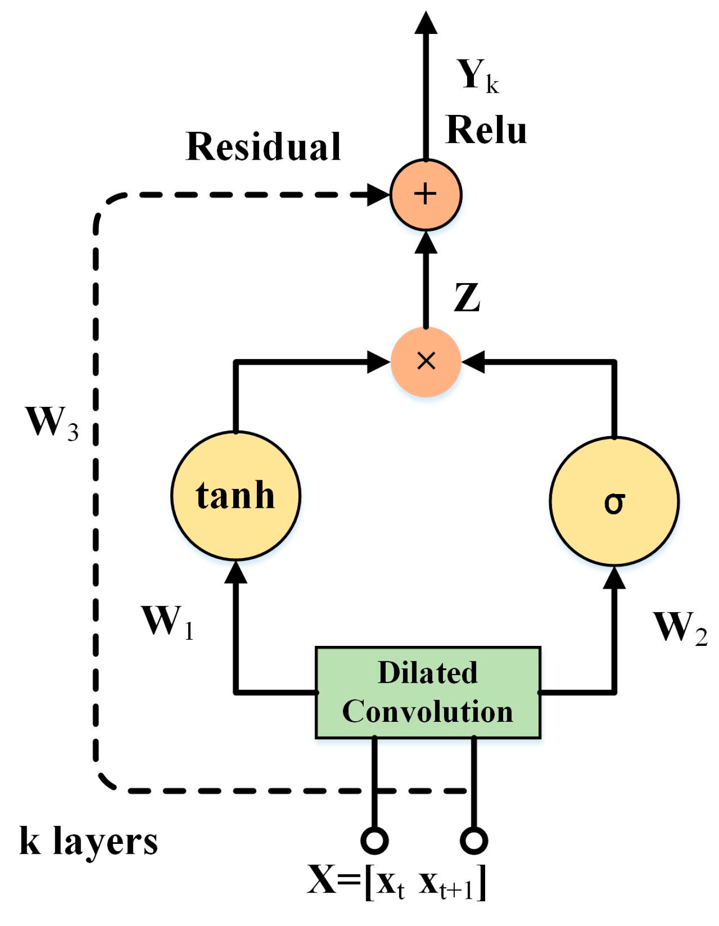
Figure 6.
Test stand for collecting vibration signals from REBs used by CWRU.

Figure 7.
Photographs of three kinds of damaged bearings.

Figure 8.
Diagram of the data augmentation.

Figure 9.
Time domain waveforms of ten types of bearing vibration signals.

Figure 10.
Diagram of the 1d-DCNN model (left) the training process and (right) confusion matrix.

Figure 11.
Diagram of the 2d-DCNN model (left) the training process and (right) confusion matrix.

Figure 12.
Diagram of the LSTM-CNN model (left) the training process and (right) confusion matrix.

Figure 13.
Diagram the SRDCNN model (left) the training process and (right) confusion matrix.

Figure 14.
Diagram of the bearing vibration signal at SNR from 2 dB to 10 dB.

Figure 15.
Results of these three methods diagnosing with noisy signal.

Figure 16.
Feature distribution visualization of noise experiment with SRDCNN model.

Figure 17.
Results of these three methods under different working loads.

Figure 18.
Feature distribution visualization of load experiment with SRDCNN model.


Table 1.
Description of all experimental datasets.
| Fault Location | None | Ball | Inner Ring | Outer Ring | Load (hp) | Speed (rpm) | |||||||
|---|---|---|---|---|---|---|---|---|---|---|---|---|---|
| Fault diameter (mil) | 0 | 7 | 14 | 21 | 7 | 14 | 21 | 7 | 14 | 21 | |||
| Dataset A | Train | 500 | 500 | 500 | 500 | 500 | 500 | 500 | 500 | 500 | 500 | 0 | 1797 |
| Test | 50 | 50 | 50 | 50 | 50 | 50 | 50 | 50 | 50 | 50 | |||
| Dataset B | Train | 500 | 500 | 500 | 500 | 500 | 500 | 500 | 500 | 500 | 500 | 1 | 1772 |
| Test | 50 | 50 | 50 | 50 | 50 | 50 | 50 | 50 | 50 | 50 | |||
| Dataset C | Train | 500 | 500 | 500 | 500 | 500 | 500 | 500 | 500 | 500 | 500 | 2 | 1750 |
| Test | 50 | 50 | 50 | 50 | 50 | 50 | 50 | 50 | 50 | 50 | |||
| Dataset D | Train | 500 | 500 | 500 | 500 | 500 | 500 | 500 | 500 | 500 | 500 | 3 | 1730 |
| Test | 50 | 50 | 50 | 50 | 50 | 50 | 50 | 50 | 50 | 50 | |||
Table 2.
Structure parameters and performance indicators of models.
| Model | 1d-DCNN | 2d-DCNN | LSTM-CNN | SRDCNN |
|---|---|---|---|---|
| Input layer | 1024 × 1 | 32 × 32 | 1024 × 1 | 1024 × 1 |
| Layer-1 | Conv1d (16 × 1, 16) | Conv2d (5 × 5, 16) | Conv1d (32 × 1, 20) | RDConv1d (64 × 1, 32) |
| Layer-2 | Pooling (2 × 1, 2) | Pooling (2 × 2, 2) | Pooling (2 × 2, 2) | RDConv1d (32 × 1, 32) |
| Layer-3 | Conv1d (3 × 1, 32) | Conv2d (5 × 5, 32) | LSTM (100) | RDConv1d (16 × 1, 64) |
| Layer-4 | Pooling (2 × 1, 2) | Pooling (2 × 2, 2) | Dense (10) | RDConv1d (8 × 1, 64) |
| Layer-5 | Conv1d (3 × 1, 64) | Flatten | Flatten | |
| Layer-6 | Pooling (2 × 1, 2) | Dense (100) | Dense (100) | |
| Layer-7 | Conv1d (3 × 1, 64) | Dense (10) | Dense (10) | |
| Layer-8 | Pooling (2 × 1, 2) | |||
| Layer-9 | Conv1d (3 × 1, 64) | |||
| Layer-10 | Pooling (2 × 1, 2) | |||
| Layer-11 | Flatten | |||
| Layer-12 | Dense (100) | |||
| Layer-13 | Dense (10) | |||
| Mean accuracy | 0.986 | 0.992 | 0.978 | 0.994 |
| Standard deviation | 0.0064 | 0.0043 | 0.0071 | 0.0015 |
Table 3.
Experiments Scenario settings for load adaptation.
| Description | Source Dataset | Target Dataset | |
|---|---|---|---|
| Dataset details | Training set B | Test set C | Test set D |
| Training set C | Test set B | Test set D | |
| Training set D | Test set B | Test set C | |
© 2019 by the authors. Licensee MDPI, Basel, Switzerland. This article is an open access article distributed under the terms and conditions of the Creative Commons Attribution (CC BY) license (http://creativecommons.org/licenses/by/4.0/).
Share and Cite
MDPI and ACS Style
Zhuang, Z.; Lv, H.; Xu, J.; Huang, Z.; Qin, W. A Deep Learning Method for Bearing Fault Diagnosis through Stacked Residual Dilated Convolutions. Appl. Sci. 2019, 9, 1823. https://doi.org/10.3390/app9091823
AMA Style
Zhuang Z, Lv H, Xu J, Huang Z, Qin W. A Deep Learning Method for Bearing Fault Diagnosis through Stacked Residual Dilated Convolutions. Applied Sciences. 2019; 9(9):1823. https://doi.org/10.3390/app9091823
Chicago/Turabian StyleZhuang, Zilong, Huichun Lv, Jie Xu, Zizhao Huang, and Wei Qin. 2019. "A Deep Learning Method for Bearing Fault Diagnosis through Stacked Residual Dilated Convolutions" Applied Sciences 9, no. 9: 1823. https://doi.org/10.3390/app9091823
Note that from the first issue of 2016, this journal uses article numbers instead of page numbers. See further details here.