Research on Robust Day-Ahead Dispatch Considering Primary Frequency Response of Wind Turbine


 ,
,
Abstract
:Featured Application
Abstract
1. Introduction
- The converter decouples the turbine’s rotor from the system frequency, which indicates that the mechanical power of the wind turbines and the electromagnetic power of the system are decoupled; in this way, the fan will not be able to provide an inertial response. Moreover, as the wind turbines usually run in a maximum power point tracking (MPPT) mode, the primary frequency reserve could not be retained;
- With a large-scale wind integrated power system taking the place of some conventional synchronous generator units with the frequency regulation capability, the inertia of the wind turbine will be 0 with no reserve in the case of frequency fluctuations due to power loss and other reasons, which will harm the inertial response ability and primary frequency reserve capacity.
2. Frequency Analysis of Wind Integrated Power System
3. Optimization Model Considering Primary Frequency Response
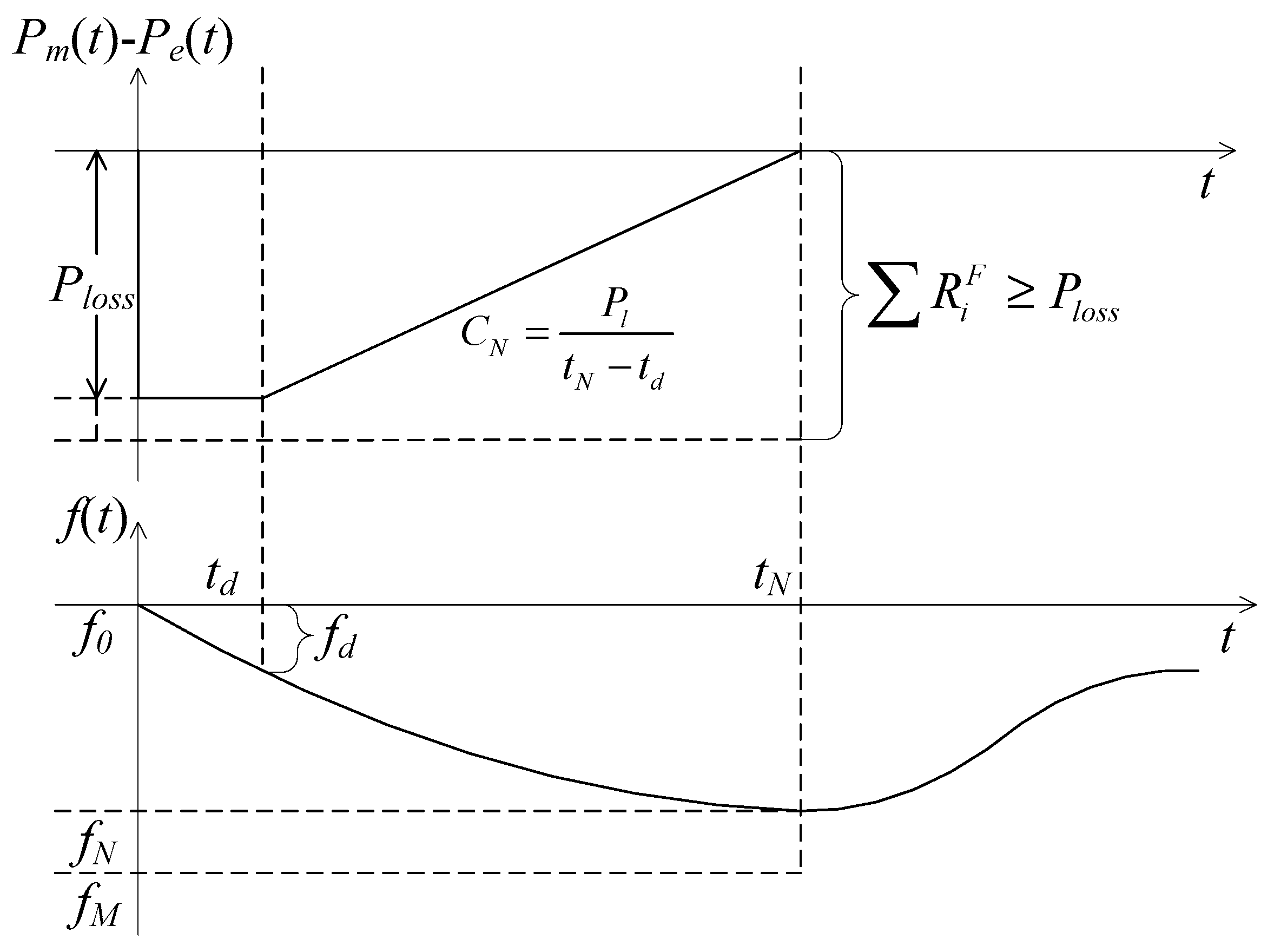
3.1. Primary Frequency Response
3.2. Two-Stage Robust Optimization Model
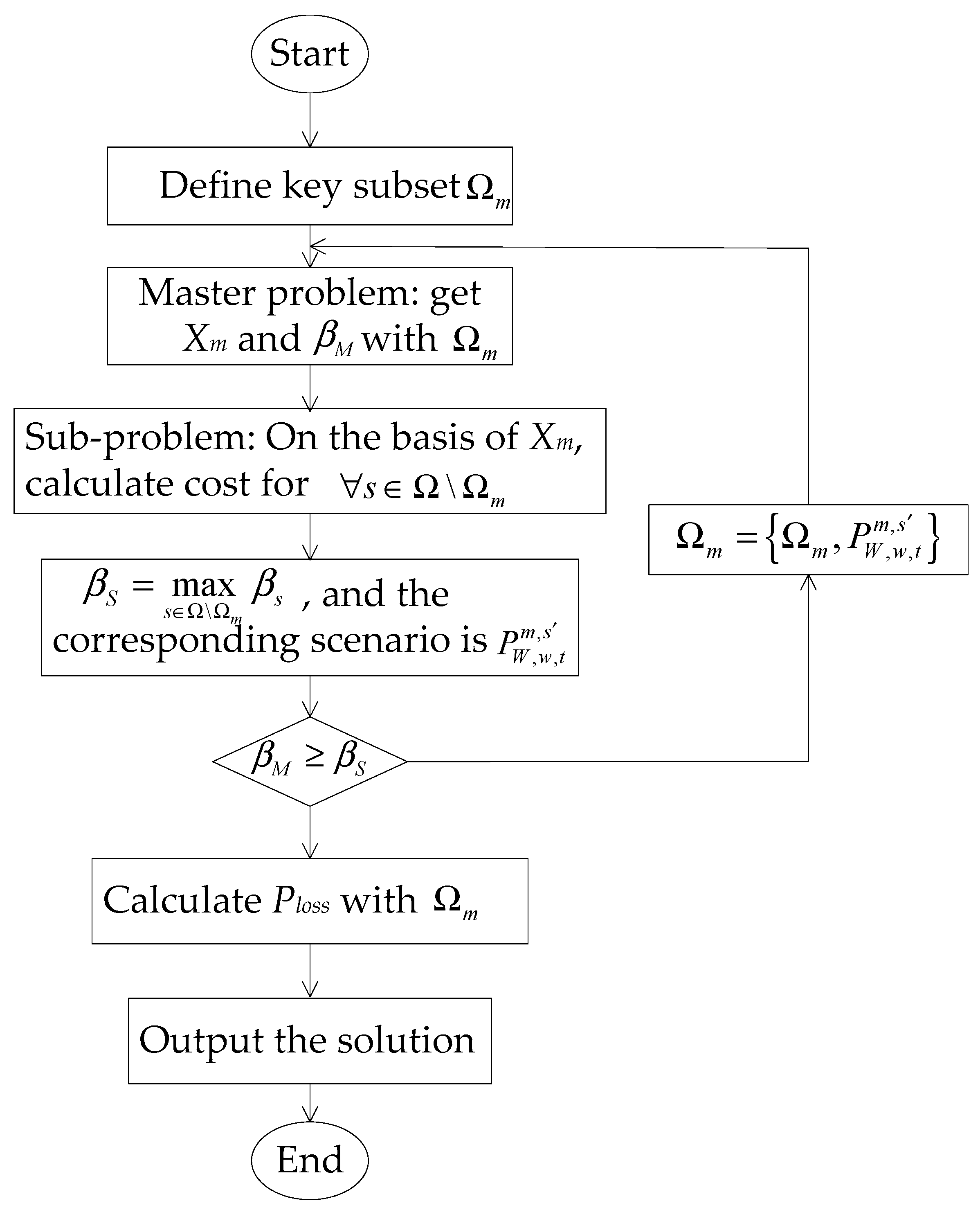
3.3. Solution
- Define the starting key subset Ωm = {};
- Master problem: solve the above model to obtain the dispatch strategy Xm and the adjustment cost βM for Stage 2;
- Sub-problem: based on Xm, calculate the goals for each and every scenario in Ω\Ωm;The optimization goal during the real-time operation is restricted by Equations (20) to (29). For the results obtained in 3, the maximum , and the corresponding scenario is ;
- If , Ωm = {Ωm, }, then we go back to 2; otherwise, we get the dispatch strategy for the master problem, and the iteration ends.
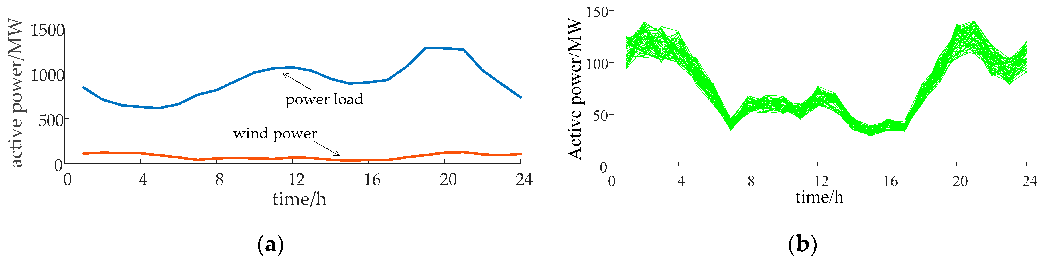
4. Results
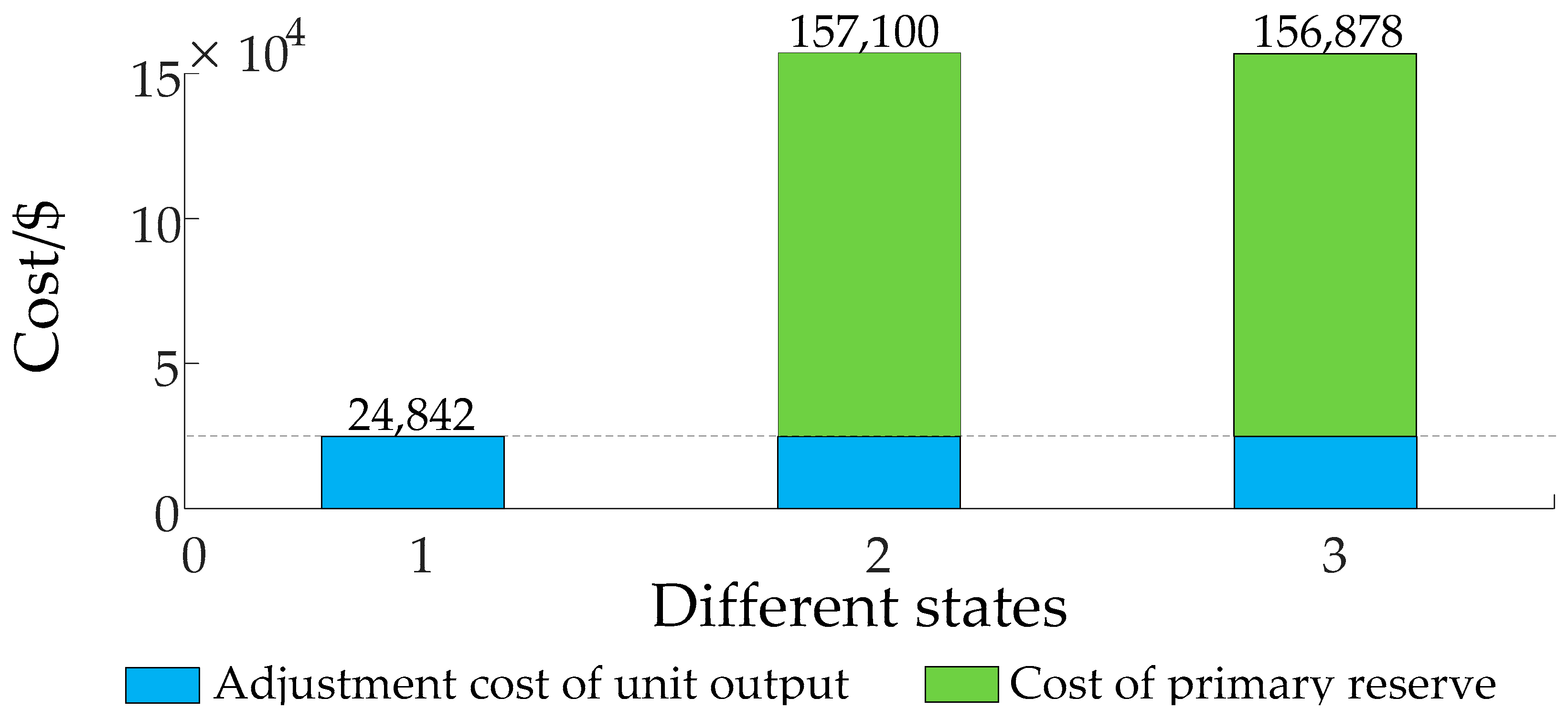
4.1. Cost Analysis
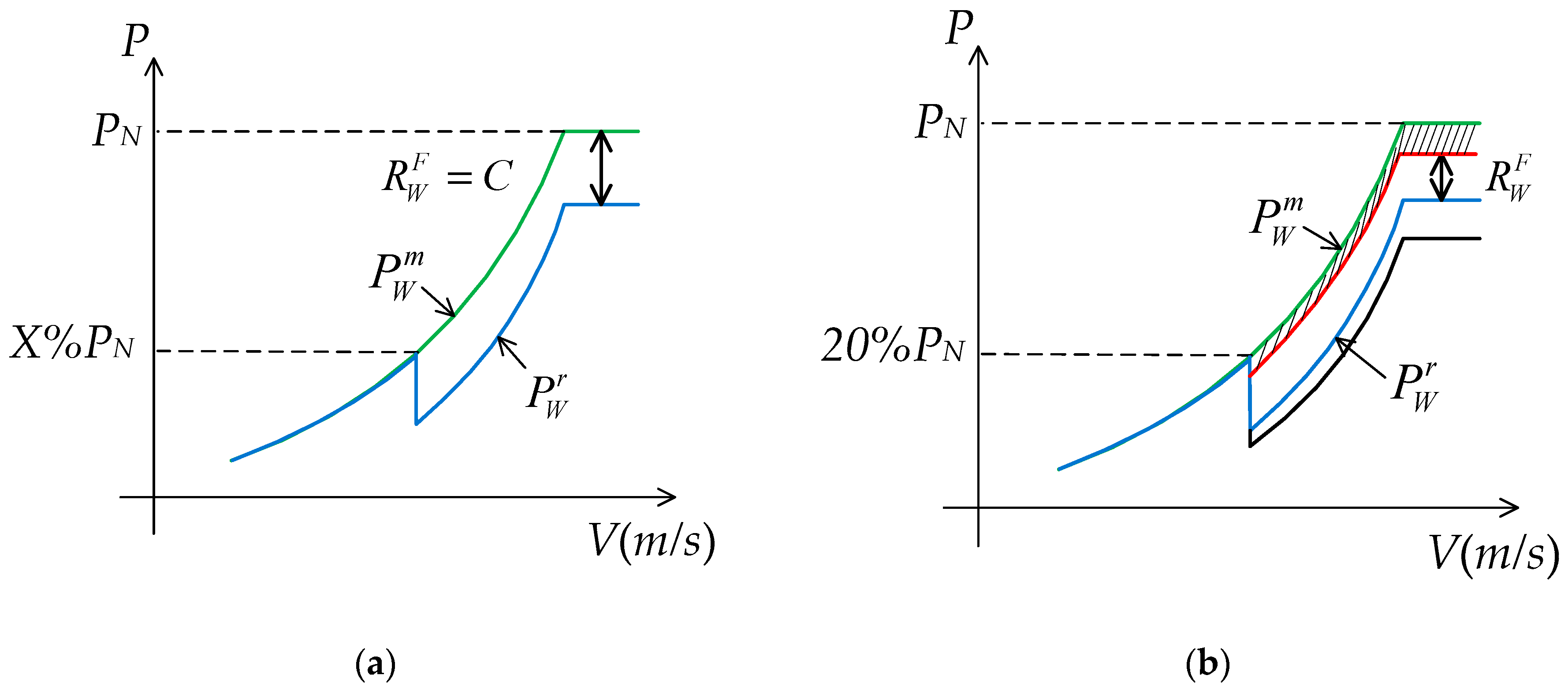
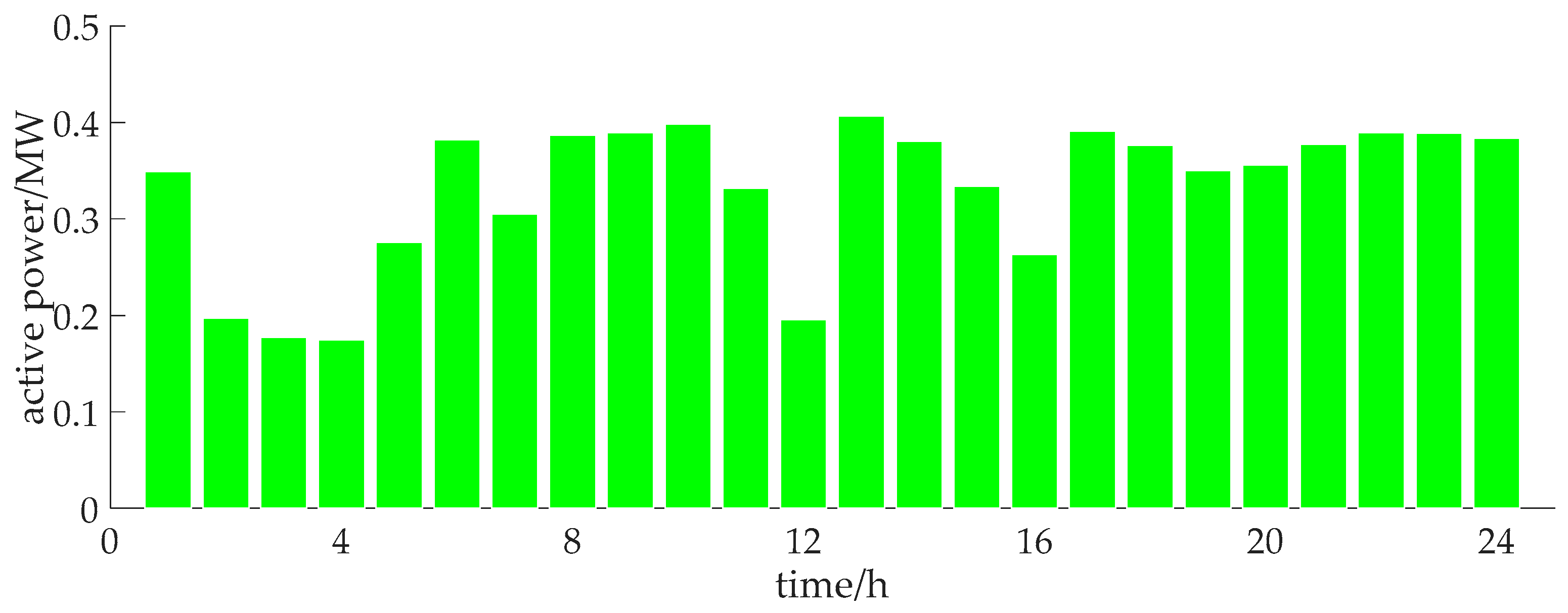
4.2. Wind Power Primary Reserve
5. Discussion
Author Contributions
Funding
Conflicts of Interest
Appendix A
- 1.
- The speed and amplitude of the primary frequency regulation are in line with certain specifications. For the thermal power units, the parameters are as follows:
- The dead band of the thermal power unit is controlled within ±0.033 Hz;
- The maximum load limit of the thermal power unit should not be less than 6% of the rated capacity of the unit;
- Response includes:
- 2.
- VSG-based independent active frequency control:
- the PFR time should be less than 3 s; and the time to reach 75% of the target load should be no more than 15 s. A complete response according to the crew response target should be done within 30 s;
- During the drop of the system frequency, the VSG should increase the active output. It should not be lower than the active output before the primary frequency regulation, and the maximum increase can be at least 10% of PN;
- During the rise of the system frequency, the VSG should cut the active output. It should not be higher than that from before the primary frequency regulation. The maximum reduction of the active output should be at least 10% of PN.
References
- Ministry of Industry Development and Environment and Resources of China Electricity Council. List of National Power Industry Statistics Bulletin in 2017. Available online: http://www.cec.org.cn/guihuayutongji/tongjxinxi/niandushuju/2018-02-05/177726.html (accessed on 17 December 2018).
- Ataee, S.; Khezri, R.; Feizi, M.R. Investigating the impacts of wind power contribution on the short-term frequency performance. In Proceedings of the Smart Grid Conference, Niroo Research Institute (NRI), Tehran, Iran, 9–10 December 2014; pp. 1–5. [Google Scholar]
- Das, K.; Müfit, A.; Hansen, A.D.; Sørensen, P.E.; Abildgaard, H. Primary reserve studies for high wind power penetrated systems. In Proceedings of the 2015 IEEE Eindhoven PowerTech, Eindhoven, The Netherlands, 29 June–2 July 2015; pp. 1–6. [Google Scholar]
- Lotfy, M.E.; Senjyu, T.; Farahat, M.A.; Abdel-Gawad, A.F.; Lei, L.; Datta, M. Hybrid Genetic Algorithm Fuzzy-Based Control Schemes for Small Power System with High-Penetration Wind Farms. Appl. Sci. 2018, 8, 373. [Google Scholar] [CrossRef]
- Yoshimoto, K.; Nanahara, T.; Koshimizu, G. Analysis of data obtained in demonstration test about battery energy storage system to mitigate output fluctuation of wind farm. In Proceedings of the CIGRE/IEEE PES Joint Symposium on Integration of Wide-Scale Renewable Resources into the Power Delivery System, Calgary, AB, Canada, 29–31 July 2009; pp. 1–5. [Google Scholar]
- Benini, M.; Canevese, S.; Cirio, D.; Gatti, A. Battery energy storage systems for the provision of primary and secondary frequency regulation in Italy. In Proceedings of the 2016 IEEE 16th International Conference on Environment and Electrical Engineering (EEEIC), Florence, Italy, 7–10 June 2016; pp. 1–6. [Google Scholar]
- Cui, Y.; Song, P.; Wang, X.S.; Yang, W.X.; Liu, H.; Liu, H.M. Wind Power Virtual Synchronous Generator Frequency Regulation Characteristics Field Test and Analysis. In Proceedings of the 2018 2nd International Conference on Green Energy and Applications (ICGEA), Singapore, 24–26 March 2018; pp. 193–196. [Google Scholar]
- Pimprikar, T.; Pawaskar, O.; Kumar, A. Virtual Synchronous Generator- A New Trend in Technology for Smart Grid Integration. In Proceedings of the 2018 International Conference on Information, Communication, Engineering and Technology (ICICET), Pune, India, 29–31 August 2018; pp. 1–5. [Google Scholar]
- Yan, X.W.; Zhang, X.Y.; Zhang, B.; Ma, Y.J.; Wu, M. Research on Distributed PV Storage Virtual Synchronous Generator System and Its Static Frequency Characteristic Analysis. Appl. Sci. 2018, 8, 532. [Google Scholar] [CrossRef]
- Jia, L.; Miura, Y.; Ise, T. Comparison of Dynamic Characteristics Between Virtual Synchronous Generator and Droop Control in Inverter-Based Distributed Generators. IEEE Trans. Power Electron. 2015, 31, 3600–3611. [Google Scholar]
- Somuah, C.B.; Schweppe, F.C. Economic Dispatch Reserve Allocation. IEEE Trans. Power Appar. Syst. 1990, 5, 2635–2642. [Google Scholar]
- Restrepo, J.F.; Galiana, F.D. Unit commitment with primary frequency regulation constraints. IEEE Trans. Power Syst. 2005, 20, 1836–1842. [Google Scholar] [CrossRef]
- Chavez, H.; Baldick, R.; Sharma, S. Governor Rate-Constrained OPF for Primary Frequency Control Adequacy. IEEE Trans. Power Syst. 2014, 29, 1473–1480. [Google Scholar] [CrossRef]
- Doherty, R.; Denny, E.; O’Malley, M. System operation with a significant wind power penetration. In Proceedings of the 2004 IEEE Power Engineering Society General Meeting, Denver, CO, USA, 6–10 June 2004; pp. 1002–1007. [Google Scholar]
- Wang, Y.; Bayem, H.; Giraltdevant, M. Methods for Assessing Available Wind Primary Power Reserve. IEEE Trans. Sustain. Energy 2015, 6, 272–280. [Google Scholar] [CrossRef]
- Das, K.; Litongpalima, M.; Maule, P.; Sørensen, P.E. Adequacy of operating reserves for power systems in future european wind power scenarios. In Proceedings of the 2015 IEEE Power & Energy Society General Meeting, Denver, CO, USA, 26–30 July 2015; pp. 1–5. [Google Scholar]
- Lorca, A.; Sun, X.A. Multistage Robust Unit Commitment with Dynamic Uncertainty Sets and Energy Storage. IEEE Trans. Power Syst. 2017, 32, 1678–1688. [Google Scholar] [CrossRef]
- An, Y.; Zeng, B. Exploring the Modeling Capacity of Two-Stage Robust Optimization: Variants of Robust Unit Commitment Model. IEEE Trans. Power Syst. 2015, 30, 109–122. [Google Scholar] [CrossRef]
- Alizadeh, M.I.; Moghaddam, P.M.; Amjady, N. Multi-stage Multi-resolution Robust Unit Commitment with Non-Deterministic Flexible Ramp Considering Load and Wind Variabilities. IEEE Trans. Sustain. Energy 2018, 9, 872–883. [Google Scholar] [CrossRef]
- Li, C.L.; Yun, J.Y.; Ding, T.; Liu, F.; Ju, Y.T.; Yuan, S. Robust Co-Optimization to Energy and Reserve Joint Dispatch Considering Wind Power Generation and Zonal Reserve Constraints in Real-Time Electricity Markets. Appl. Sci. 2017, 7, 680. [Google Scholar] [CrossRef]
- Ding, T.; Liu, S.; Yuan, W.; Bei, Z.H.; Zeng, B. A Two-Stage Robust Reactive Power Optimization Considering Uncertain Wind Power Integration in Active Distribution Networks. IEEE Trans. Sustain. Energy 2016, 7, 301–311. [Google Scholar] [CrossRef]
- Samimi, A.; Kazemi, A. A New Approach to Optimal Allocation of Reactive Power Ancillary Service in Distribution Systems in the Presence of Distributed Energy Resources. Appl. Sci. 2015, 5, 1284–1309. [Google Scholar] [CrossRef]
- Chen, S.; Wei, Z.; Sun, G.; Cheung, K.; Wang, D.; Zang, H. Adaptive Robust Day-ahead Dispatch for Urban Energy Systems. IEEE Trans. Ind. Electron. 2019, 66, 1379–1390. [Google Scholar] [CrossRef]
- Li, X.; Chen, G. Improved Adaptive Inertia Control of VSG for Low Frequency Oscillation Suppression. In Proceedings of the 2018 IEEE International Power Electronics and Application Conference and Exposition (PEAC), Shenzhen, China, 4–7 November 2018; pp. 1–5. [Google Scholar]
- Hua, X.; Hongyuan, X.; Na, L. Control strategy of DFIG wind turbine in primary frequency regulation. In Proceedings of the 2018 13th IEEE Conference on Industrial Electronics and Applications (ICIEA), Wuhan, China, 31 May–2 June 2018; pp. 1751–1755. [Google Scholar]
- Sharma, S.; Huang, S.H.; Sarma, N. System inertial frequency response estimation and impact of renewable resources in ERCOT interconnection. In Proceedings of the 2011 IEEE Power and Energy Society General Meeting, Detroit, MI, USA, 24–29 July 2011; pp. 1–6. [Google Scholar]
- Transmission Provider Technical Requirements for the Connection of Power Plants to the Hydro-Québec Transmission System; Hydro-Québec TransÉnergie: Quebec, QC, Cananda, 2009.
- Grid Code Documents Connection Conditions; National Grid (Great Britain) Company: London, UK, 2009.
- Milligan, M.; Donohoo, P.; Lew, D.; Ela, E.; Kirby, B.; Holttinen, H.; Lannoye, E.; Flynn, D.; O’Malley, M.; Miller, N.; et al. Operating reserves and wind power integration: An international comparison. In Proceedings of the 9th Annual International Workshop on Large—Scale Integration of Wind Power into Power Systems as well as on Transmission Networks for Offshore Wind Power Plants Conference, Québec, QC, Canada, 18–19 October 2010; pp. 1–19. [Google Scholar]
- Parnianifard, A.; Azfanizam, A.S.; Ariffin, M.K.A.; Ismail, M.I.S. An overview on robust design hybrid metamodeling: Advanced methodology in process optimization under uncertainty. Int. J. Ind. Eng. Comput. 2018, 9, 1–32. [Google Scholar] [CrossRef]
- Soares, T.; Bessa, R.J.; Pinson, P.; Morais, H. Active distribution grid management based on robust ac optimal power flow. IEEE Trans. Smart Grid 2018, 9, 6229–6241. [Google Scholar] [CrossRef]
- Chassin, D.P.; Huang, Z.; Donnelly, M.K.; Hassler, C.; Ramirez, E.; Ray, C. Estimation of the WECC System Inertia Using Observed Frequency Transients. IEEE Trans. Power Syst. 2004, 20, 1190–1192. [Google Scholar] [CrossRef]
- Inoue, T.; Taniguchi, H.; Ikeguchi, Y.; Yoshida, K. Estimation of Power System Inertia Constant and Capacity of Spinning-Reserve Support Generators Using Measured Frequency Transients. IEEE Trans. Power Syst. 1997, 12, 136–143. [Google Scholar] [CrossRef]
- Elkraft System; Eltra. Wind turbine connected to grids with voltage above 100 kV; Technical Regulation TF 3.2.5; Danish Energy Authority: Copenhagen, Denmark, 2004; pp. 1–22. [Google Scholar]
- Bertsimas, D.; Litvinov, E.; Sun, X.A.; Zhao, J.; Zheng, T. Adaptive robust optimization for the security constrained unit commitment problem. IEEE Trans. Power Syst. 2013, 28, 52–63. [Google Scholar] [CrossRef]
- LÖFBERG, J. YALMIP: A toolbox for modeling and optimization in MATLAB. In Proceedings of the 2004 IEEE International Conference on Robotics and Automation, New Orleans, LA, USA, 2–4 September 2004; pp. 284–289. [Google Scholar]


| Key Subset Ωm | Cost/$ | ||
|---|---|---|---|
| Without Primary Reserve | PFR not Involving the Wind Power | PFR Involving the Wind Power | |
| {6;49} | 5,375,256 | 5,508,326 | 5,508,085 |
| Cost Coefficient/($/MW) | Cost/$ | Primary Reserve Capacity of Wind Power Units/MW | Cost Coefficient/($/MW) | Cost/$ | Primary Reserve Capacity of Wind Power Units/MW |
|---|---|---|---|---|---|
| 0 | 5,513,209 | 10.9061 | 200 | 5,513,664 | 9.6847 |
| 100 | 5,513,436 | 10.5484 | 300 | 5,513,891 | 8.2178 |
© 2019 by the authors. Licensee MDPI, Basel, Switzerland. This article is an open access article distributed under the terms and conditions of the Creative Commons Attribution (CC BY) license (http://creativecommons.org/licenses/by/4.0/).
Share and Cite
Sun, R.; Chen, B.; Lv, Z.; Mei, J.; Zang, H.; Wei, Z.; Sun, G. Research on Robust Day-Ahead Dispatch Considering Primary Frequency Response of Wind Turbine. Appl. Sci. 2019, 9, 1784. https://doi.org/10.3390/app9091784
Sun R, Chen B, Lv Z, Mei J, Zang H, Wei Z, Sun G. Research on Robust Day-Ahead Dispatch Considering Primary Frequency Response of Wind Turbine. Applied Sciences. 2019; 9(9):1784. https://doi.org/10.3390/app9091784
Chicago/Turabian StyleSun, Rong, Bing Chen, Zhenhua Lv, Jianchun Mei, Haixiang Zang, Zhinong Wei, and Guoqiang Sun. 2019. "Research on Robust Day-Ahead Dispatch Considering Primary Frequency Response of Wind Turbine" Applied Sciences 9, no. 9: 1784. https://doi.org/10.3390/app9091784
APA StyleSun, R., Chen, B., Lv, Z., Mei, J., Zang, H., Wei, Z., & Sun, G. (2019). Research on Robust Day-Ahead Dispatch Considering Primary Frequency Response of Wind Turbine. Applied Sciences, 9(9), 1784. https://doi.org/10.3390/app9091784