A Bilateral Tradeoff Decision Model for Wind Power Utilization with Extensive Load Scheduling

Featured Application

We present an improved methodology for increasing the wind power utilization by responsive loads; the consumption of wind power and cost of system operation are optimized simultaneously through the multi-objective differential evolution method. The responsive loads are divided into two kinds according to their response characteristic and the randomness of wind power are considered by chance constraint. The proposed methodology can maximize the wind power utilization and minimize the system operation cost more effectively.

Abstract

In this paper, we present the extensive load scheduling problem with intermittent and uncertain wind power availability. A chance-constrained bilateral tradeoff decision model is established to solve the problem. Our model aims at maximizing the wind power utilization and minimizing the system operation cost simultaneously by means of responsive loads, which are precisely divided into shiftable loads and high-energy loads. The chance constraint is applied to restrict the system imbalance with a small probability. Then, a revised sample average approximation (SAA) algorithm is developed to transform the chance constraint into sample average reformulations. Furthermore, the multi-objective differential evolution (MODE) method combined with SAA is proposed to solve the problem. Experiments enabling an effectiveness analysis of the two kinds of responsive loads are performed on the power system in Yancheng. The research of parameters of MODE, the sensitivity of different risk levels and the influence of iteration numbers are discussed. Finally, computational results prove that the combination of shiftable loads and high-energy loads have a better effect than adopting shiftable loads and high-energy loads separately, and the proposed method is convergent and valid in solving the problem.

1. Introduction

Wind power, which is clean and renewable, has been integrated with the grid on a large scale to replace fossil fuels [1,2]. A lot of countries have set goals for high-penetration wind power levels in the grid to increase the wind power utilization. China aims to achieve an average wind power utilization rate of 95% in 2020. However, the randomness and intermittence of wind power have increased the tremendous challenges in wind energy utilization as well as the power system operators and planners [3,4]. The traditional dispatching operating mode of a power system, designed to address limited uncertainty in the system, encounters challenges in accommodating the high penetration of large-scale wind power. Thus, new methods should be developed to cope with the situation [5].

The chance-constrained optimization technique has been adopted to manage the problems involved stochastic variables in some previous studies [6,7]. In [7], the chance constraints in the optimization formulations guarantees that the failure probability of the EV charging plan fulfilling the driving requirement is below the predetermined confidence parameter. In [6], a chance constrained programing approach was presented to ensure desired confidence levels of meeting future stochastic power and natural gas demands while minimizing the investment cost. In the present study, the chance constraint is applied to ensure the probability of system imbalance caused by too little system reserve capacity is less than a certain probability. These types of constraints could not be inverted to obtain equivalent deterministic equalities. Thus, the method developed in [7] could not be directly applied here to solve our problem. In addition, the joint chance constrained problem in [6] are formulated through mixed-integer quadratic programming (MIQP), which is not efficient method to solve our problem related to not joint chance constraints. Therefore, we propose the sample average approximation (SAA) algorithm [8] to solve the problem. The approach can provide a solution that converges to the optimal one as the number of samples increases.

During the Spring Festival, the load is expected to drop sharply which will decrease the usage of power. In 2018, to ensure the safe and stable operation of the power grid, Shandong Electric Power Company took measures to limit renewable energy output, which means that a large amount of wind power would be abandoned. However, Jiangsu Electric Power Company actively encourages enterprises to produce, which not only increases the load of 9000 MW for trough load periods but also promotes the consumption of renewable energy. In the first three days of the Spring Festival, a total of 72000 MWh of renewable energy consumption was added. In the smart grid, the load, as an important responsive resource [9,10], is an excellent alternative for wind power consumption [11,12].

Extensive research has been done to increase wind power utilization through the participation of responsive loads. In [13], a model for solving the combined effect of PEVs and wind power integration with a DR (demand response) program on static transmission network expansion planning was proposed, but the uncertainty of wind power has not been considered. A two-stage stochastic model which handling the forecast errors of renewable generations in a microgrid with responsive loads was implemented in [14], however, the objective of the model is only operation cost not including the renewable energy utilization. Hajibandeh Neda [15] investigated the potential of DR as an emerging alternative in systems with significant amounts of wind power. A comprehensive set of DR programs including tariff-based, incentive-based and combinational DR programs are considered in a stochastic network-constrained market clearing framework. Kalavani Farshad [16] provided a stochastic method to conduct the optimal scheduling of the combination of wind power and energy storage with considering the DR program in the electricity market. The DR program was adopted to increase the total expected profit and decrease the total operational cost.

Most models in this context have optimized wind power utilization by responsive loads. However, the scheduling characteristics of loads were not considered, and responsive loads were not divided finely. Different types of responsive loads have different characteristics [17]. Therefore, different loads can participate in the optimized operation in different ways [18], which may lead to better optimized results.

In this study, according to their regulating characteristics, loads are grouped into two types, including the high-peneration energy load (HL) and the shiftable load (SL). The HL possesses both adjustable and interruptible characteristics, which can achieve power control in the range of 0%–100%. The regulate action can be completed in an instant. The HL is suitable for increasing wind power consumption because we can raise its power when the wind power is high and reduce its power in the opposite case. The use of an SL implies shifting the load from one period to another to maintain the electricity consumption. Loads can be cut out or put in at any periods of the whole cycle. Generally, an SL is put in during the peak wind power periods and cut out in trough wind power periods to increase the wind power utilization. HLs and SLs are shown in Figure 1.

The two types of responsive load participate in the optimal scheduling with conventional power, developing a new scheduling mode based on source-load coordinate optimal operation. However, the dispatch of responsive loads will damage the users’ benefit. Economic compensation needs to be made for them, which incurs additional costs. Thus, besides the amount of consumption of wind power, the cost of system operation should be considered as well. The model contains two objectives: to obtain the maximum capacity of wind power accommodation and to minimize the system operation costs. A multi-objective optimal model is established in this study.

There are many algorithms that can be used to solve the multi-objective optimal problem, for example: the Non-dominated sorting genetic algorithm II (NSGA-II) [19], the Strength pareto evolutionary algorithm (SPEA) [20], the Pareto archived evolution strategy (PAES) [21] and the Multi-objective differential evolution (MODE) [22]. In [19], NSGA-II, SPEA2 and PAES were designed for multi-objective problems, and NSGA-II achieved the best results in terms of Pareto front spread. 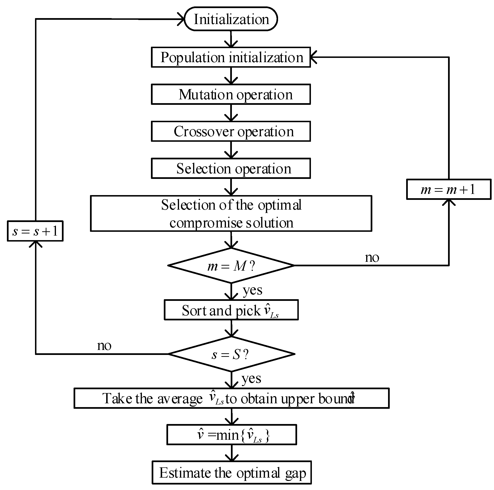In [22], NSGA-II, MODE and multi-objective particle swarm optimization (MOPSO) algorithms are compared in accuracy and computational time. The results show that the obtained Pareto Front of MODE is more accurate and faster. It can be concluded that MODE performs better among these algorithms. So we adopted MODE algorithm to solve the multi-objective model in this paper.

The remaining part of this paper is organized as follows. Section 2 describes the problem with chance constraints. Section 3 presents the solution methods which including SAA and MODE algorithms. Section 4 reports the computational experiments for the power system of Yancheng City of Jiangsu province in China. Section 5 concludes the study.

2. Problem Description

In this section, we develop a chance-constrained multi-objective formulation to address uncertain wind power availability. The two objectives are to maximize the utilization of wind power $E_W$ and to minimize the system operation cost $C_{GL}$, which including the costs of thermal generator and the operation costs of SLs and HLs. HLs and SLs are adopted in the optimization. The formulation is to determine the regulate or shift operations of the responsive loads. The detailed formulation is shown as follows:

$$\{\begin{array}{l}\max E_W={\displaystyle \sum _{t=1}^T{\displaystyle \sum _{i=1}^{N_W}{P}_{Wi}^t}\Delta T}\hfill \\ \min C_{GL}=C_{gen}+C_{SL}+C_{HL}\hfill \end{array}$$

(1)

$s.t.$

$${\displaystyle \sum _{j=1}^{N_G}{u}_{Gj}^t{P}_{Gj}^t}+{\displaystyle \sum _{i=1}^{N_W}{P}_{Wi}^t}=P_L^t+{\displaystyle \sum _{a=1}^{N_S}{S}_{Sa}^t{P}_{Sa}^t}+{\displaystyle \sum _{b=1}^{N_I}{S}_{Hb}^t{P}_{Hb}^t}, t\in T$$

(2)

$${\displaystyle \sum _{j=1}^{N_G}{u}_{Gj}^t(P_{Gj}^{\max }-P_{Gj}^t})\ge R_L^t+\gamma {\displaystyle \sum _{i=1}^{N_W}{P}_{Wi}^t}, t\in T$$

(3)

$$u_{Gj}^t{P}_{Gj}^{\min }\le P_{Gj}^t\le u_{Gj}^t{P}_{Gj}^{\max }, j\in G, t\in T$$

(4)

$$\begin{array}{l}-u_{Gj}^{t-1}+u_{Gj}^t-u_{Gj}^k\le 0;\\ (1\le k-(t-1)\le T_{Gj,on}^{\min },j\in G, t\in T)\end{array}$$

(5)

$$\begin{array}{l}{u}_{Gj}^{t-1}-u_{Gj}^t+u_{Gj}^k\le 1;\\ (1\le k-(t-1)\le T_{Gj,off}^{\min },j\in G, t\in T)\end{array}$$

(6)

$$\begin{array}{l}{P}_{Gj}^t-P_{Gj}^{t-1}\le (2-u_{Gj}^{t-1}-u_{Gj}^t)P_{Gj}^{\max }+(1+u_{Gj}^{t-1}-u_{Gj}^t)R_{Gj}^{up}\\ (j\in G, t\in T)\end{array}$$

(7)

$$\begin{array}{l}{P}_{Gj}^{t-1}-P_{Gj}^t\le (2-u_{Gj}^{t-1}-u_{Gj}^t)P_{Gj}^{\max }+(1-u_{Gj}^{t-1}+u_{Gj}^t)R_{Gj}^{down}\\ (j\in G,t\in T)\end{array}$$

(8)

$$0\le P_{Wi}^t\le P_{Wi}^{\max }i\in W, t\in T$$

(9)

$$\mathrm{Pr}\left\{P_{Wi}^t-\gamma P_{Wi}^t\le {\zeta }_{wi}^t\right\}\ge 1-\epsilon i\in W, t\in T$$

(10)

$$-{\mathrm{S}}_{Sa}^t{P}_{Sa\max }^t\le P_{S,a}^t\le {\mathrm{S}}_{Sa}^t{P}_{Sa\max }^{t}a\in SL, t\in T$$

(11)

$${\displaystyle \sum _{t=1}^T{S}_{Sa}^t{P}_{Sa}^t}=0, a\in Sa$$

(12)

$$0\le P_{H,b}^t\le {\mathrm{S}}_{Hb}^t{P}_{Hb\max }^t \mathrm{b}\in HL, t\in T$$

(13)

$$\begin{array}{l}-S_{Sa}^{t-1}+S_{Sa}^t-S_{Sa}^k\le 0;\\ (1\le k-(t-1)\le T_{Sa,on}^{\min }, a\in SL)\end{array}$$

(14)

$$\begin{array}{l}-S_{Hb}^{t-1}+S_{Hb}^t-S_{Hb}^k\le 0\\ (1\le k-(t-1)\le T_{Hb,on}^{\min },b\in HL)\end{array}$$

(15)

$$0\le {\displaystyle \sum _{t=1}^T\left|S_{Sa}^t-S_{Sa}^{t-1}\right|}\le M_{Sa}, a\in SL$$

(16)

$$0\le {\displaystyle \sum _{t=1}^T\left|S_{\mathrm{H}b}^t-S_{\mathrm{H}b}^{t-1}\right|}\le M_{Hb},b\in HL$$

(17)

$$-P_{ij}^{\max }\le b_{ij}\cdot ({\theta }_i-{\theta }_j)\le P_{ij}^{\max } (j\in i,j\ne i,\forall i)$$

(18)

$$P_G-P_L=-B^{\prime }\theta$$

(19)

where

$$C_{gen}={\displaystyle \sum _{t=1}^T{\displaystyle \sum _{j=1}^{N_G}\{u_{Gj}^t[l_j+m_j{P}_{Gj}^t+n_j{(P_{Gj}^t)}^2]\Delta T+[u_{Gj}^t(1-u_{Gj}^{t-1})+(1-u_{Gj}^t)u_{Gj}^{t-1}]{\lambda }_{Gj}\}}}$$

(20)

$$C_{SL}={\displaystyle \sum _{t=1}^T{\displaystyle \sum _{a=1}^{N_S}{\lambda }_{Sa}{S}_{Sa}^t{P}_{Sa}^t\Delta T}}$$

(21)

$$C_{HL}={\displaystyle \sum _{t=1}^T{\displaystyle \sum _{b=1}^{N_H}{\lambda }_{Hb}{S}_{Hb}^t{P}_{Hb}^t\Delta T}}$$

(22)

In the above formulation, the functions (1) represents the two objectives. One is to maximize utilization of wind power; the other is to minimize the system operation cost, which is composed of the generation cost of thermal generators $C_{gen}$, the operation cost of shiftable loads $C_{SL}$ and the operation cost of high-energy loads $C_{HL}$. Constraint (2) represents the power balance of the system. $P_L^t$ is the total amount of conventional system load over time period $t$ which doesn’t include SL and HL. Constraint (3) describes that the reserve needed for loads forecast error and wind power forecast error should be satisfied. Constraint (4) limits the upper and lower bounds of power generation of each unit. Constraints (5) and (6) mean the status (on or off) of each unit must last for a minimum time once it is started up or shut down. Constraints (7) and (8) are the unit ramping up constraints and ramping down constraints respectively. Constraint (9) represents that the utilization of wind power cannot exceed the maximum value. Chance-constraint (10) means that the probability of system imbalance caused by the too little system reserve capacity is less than risk level $\epsilon$. Constraints (11) and (13) indicate the SLs and HLs must be less than or equal to the schedulable capacity. Constraint (12) show that the total power consumption of each shiftable load can’t change. Constraints (14) and (15) describe the use of SLs and HLs should exceed a certain minimum time. Constraints (16) and (17) describe the limitation of the dispatched numbers of each SL and HL. Constraint (18) represents the transmission capacity constraints of each line. Constraint (19) is the formula of DC power flow calculation.

Equalities (20), (21) and (22) describe the costs of thermal generator and the operation costs of SLs and HLs.

To sum up, the bilateral tradeoff model can be described as (23). $F=(-E_W,C_{GL})$ is the objective function for this study. $\mathit{x}$ is a decision variable. $f_j(\mathit{x})$ is the equality constraint function, and $g_k(\mathit{x})$ is the inequality constraint function.

$$\{\begin{array}{l}\min F(\mathit{x}),\hfill \\ \mathrm{s}.\mathrm{t}. \{\begin{array}{l}{f}_j(\mathit{x})=0, j=1\hfill \\ g_k(\mathit{x})\le 0, k=1,2,\cdots ,n\hfill \end{array}\hfill \end{array}$$

(23)

3. Solution Method

3.1. Revised Sample Average Approximation

SAA is an effective method to solve the chance-constrained problem. The basic idea of SAA is to approximate the true distribution of random variables with an empirical distribution through Monte Carlo sampling technology. Multiple theoretical research studies and computational studies of SAA have been developed for chance-constrained stochastic problems [23]. In this section, we develop a combined SAA algorithm to solve the chance-constrained program. The combined SAA framework contains three parts: scenario generation, convergence analysis and solution validation.

3.1.1. Scenario Generation

The wind power availability is closely related to the wind speed. Recently, a variety of theoretical distributions were proposed to fit the probability distribution of wind speed [24]. In the present study, we adopt two-parameter Weibull distribution to fit the probability distribution of actual wind speed. The Monte Carlo simulation is run to generate N scenarios of the wind power random variable ${\zeta }_{wi}^{t,n}$, and each scenario has the same probability of 1/N. $1_{(0,\infty )}(\cdot )$ is an indicator function, i.e.,

$$1_{(0,\infty )}(t)=\{\begin{array}{l}1 t>0\\ 0 t\le 0\end{array}$$

(24)

The chance constraints (10) can be replaced by

$${\widehat{P}}_N(x)=\frac{1}{N}{\displaystyle \sum _{n=1}^N{1}_{(0,\infty )}}(p_{wi}^t-\beta p_{wi}^t-{\zeta }_{wi}^{t,n})\le \delta$$

(25)

First, if $\delta =\epsilon$, as the sample size N goes to infinity, we can prove that the solution of the SAA problem converges to the solution of the true problem. Since N cannot be infinity, it is possible that the solution of the SAA problem is infeasible with respect to the true problem. To increase the confidence level for the solution of SAA problem to be feasible, we let $\delta <\epsilon$. Generally, and $N=2/\epsilon ,\delta =\epsilon /2$.

3.1.2. Solution Validation

Assume that $\widehat{x}$ is the solution of the SAA problem and that $\widehat{v}$ is the corresponding value of objective function. To test the feasibility of $\widehat{x}$, we construct the upper bound of $\widehat{v}$.

First, S iterations were taken. For each iteration, we run the SAA problem M times with N scenarios. As described in [23], we let L be the largest integer to meet the constraint (27).

$${\theta }_N=B(\delta N; \epsilon ,N)$$

(26)

$$B(L-1; {\theta }_N,M)\le \omega$$

(27)

With $B$ denoting the binomial distribution. Then, selecting the Lth smallest optimal value denoted as ${\widehat{v}}_{Ls}$, the confidence level for ${\widehat{v}}_{Ls}$ to be the upper bound of the chance-constrained problem is more than $1-\omega$. The average of ${\widehat{v}}_{L1},{\widehat{v}}_{L2},\dots ,{\widehat{v}}_{LS}$ is the upper bound; the smallest one of ${\widehat{v}}_{L1},{\widehat{v}}_{L2},\dots ,{\widehat{v}}_{LS}$ is the optimal value ${\tilde{v}}_o$.

3.1.3. Summary of the SAA Algorithm

The proposed SAA algorithm is summarized in the following steps.

(1)

For $s=1,2,\cdots S$, repeat steps ①–②.

① For $m=1,2,\cdots M$, repeat steps i-ii.

i. Generate $N$ scenarios of the random vector $\zeta$;

ii. Solve the proposed model by MODE to obtain the solution as $\widehat{x}$ and the objective value as $\widehat{v}$.

② Sort the $M$ optimal values in an ascending order, and denote the Lth value ${\widehat{v}}_L$ as ${\widehat{v}}_{Ls}$.

(2)

The upper bound is defined as $\widehat{v}=\frac{1}{S}{\displaystyle \sum _{s=1}^S{\widehat{v}}_{Ls}}$, and the minimum value from ${\widehat{v}}_{L1}$ to ${\widehat{v}}_{Ls}$ is taken as the optimal objective value ${\tilde{v}}_o$. The corresponding optimal solution $\widehat{x}$ can also be obtained.

(3)

Calculate the optimality gap by $(\widehat{v}-{\tilde{v}}_o)/{\tilde{v}}_o\times 100\%$.

3.2. Multi-Objective Differential Evolution

The problem is a multi-objective mixed-integer linear program (MILP) [25], which cannot be solved by CPLEX. CPLEX can provide flexible high-performance optimization programs to solve the single-objective problems, which including linear programming problem, quadratic programming problem and mixed-integer programming problem. However, it is not applicable in multi-objective problems. Hence, MODE algorithm was proposed in this paper. Because of the dual objectives, a set of Pareto optimal solutions would be obtained. Therefore, a novel fuzzy membership function [26] is introduced to select the optimal compromise solution from Pareto solution set.

3.2.1. Multi-Objective Differential Evolution

MODE is a type of random parallel direct global search algorithm with the advantages of simple and easy-to-use global optimization. Its details are as follows:

(1)

Population initialization: The initial population $X_0$ is chosen arbitrarily in the solution space, and the population scale number is $N_p$.

(2)

Mutation operation: The variation operation is based on the difference of random sampling individuals as follows:

$${\mathit{v}}_{i,G+1}={\mathit{x}}_{r1,G}+F\times ({\mathit{x}}_{r2,G}-{\mathit{x}}_{r3,G})$$

(28)

where $G$ is the evolution times, ${\mathit{v}}_{i,G+1}$ is a variation individual and ${\mathit{x}}_{r1,G}$ is the father individual. $({\mathit{x}}_{r2,G}-{\mathit{x}}_{r3,G})$ is the father difference vector, and $r1\ne r2\ne r3\ne i$. $F$ is a control parameter that satisfies $F\in [0,1]$.

(3)

Crossover operation: Once the perturbed individual ${\mathit{v}}_{i,G+1}$ is generated, this individual is subjected to crossover operation with a target individual ${\mathit{X}}_{i,G+1}$ that ultimately generates the trial solution,${\mathit{u}}_{i,G+1}$, as follows:

$${\mathit{u}}_{ij,G+1}=\{\begin{array}{ll}{\mathit{v}}_{ij,G+1},& ran{d}_j()\le Cr or j=j_{rand}\\ {\mathit{u}}_{ij,G},& otherwise\end{array}$$

(29)

(4)

Selection operation: We make a temporary population ${\mathit{X}}^{\ast }$ and then let the test individual ${\mathit{z}}_{i,G+1}$ compete with the father individual ${\mathit{x}}_{i,G}$. The better one would be selected to ${\mathit{X}}^{\ast }$ [27].

3.2.2. Selection of the Optimal Compromise Solution

To obtain the balance of wind power cost and economical operation of the system, we need to measure the membership of each Pareto solution and use this measurement to find the optimal compromise solution. In this study, we introduce a novel fuzzy membership function as follows:

$$u_i=\frac{f_{i\max }-f_i}{f_{i\max }-f_{i\min }}$$

(30)

where $f_{i\max }$ and $f_{i\min }$ are the upper and lower bound of the $i\mathrm{th}$ objective function, respectively. The standard membership degree is estimated as $u={\displaystyle \sum _{i=1}^2{u}_i}$. The largest membership is corresponding to the optimal compromise solution. The flowchart of the SAA algorithm combined with MODE is shown in Figure 2.

4. Results and Discussion

In this section, we conduct a series of experiments on the power system of Yancheng in Jiangsu, China to illustrate the proposed approach. The advantages of dual-objective model and the impact of SLs and HLs are manifested. We also discuss the sensitivity of risk level and the convergence of the proposed SAA algorithm combined with MODE. The time horizon was 24 h at 0.5 h step. The relevant information can be obtained from the state grid corporation.

4.1. Introduction of the Yancheng Power System

Yancheng, with six wind farms, has abundant wind power resources. The topological structure of the Yancheng power system is shown in Figure 3. The specific information of HLs and SLs is shown in the

Table 1. Parameters of high-energy load users.

Load Type	Location	Number	${\mathit{P}}_{\mathit{H}\mathit{b}}$ (MW)	${\mathit{P}}_{\mathit{H}\mathit{max}}$ (MW)	${\mathit{\lambda }}_{\mathit{H}}$ ($/MWh)	${\mathit{M}}_{\mathit{H}\mathit{b}}$	${\mathit{T}}_{\mathit{H}\mathit{b},\mathit{o}\mathit{n}}^{\mathit{min}},{\mathit{T}}_{\mathit{H}\mathit{b},\mathit{o}\mathit{f}\mathit{f}}^{\mathit{min}}$
Beneficiation	Binhai	13	10	130	60	3	1
Chemical engineering	Funing	10	6	60	65	3	1
Industrial engineering	Dongtai	8	10	80	55	3	1

and

Table 2. Parameters of Shiftable load users.

Load Type	Location	Number	${\mathit{P}}_{\mathit{S}\mathit{a}}$ (MW)	${\mathit{P}}_{\mathit{S}\mathit{max}}$ (MW)	${\mathit{\lambda }}_{\mathit{S}}$ ($/MWh)	${\mathit{M}}_{\mathit{S}\mathit{a}}$	${\mathit{T}}_{\mathit{S}\mathit{a},\mathit{o}\mathit{n}}^{\mathit{min}}, {\mathit{T}}_{\mathit{S}\mathit{a},\mathit{o}\mathit{f}\mathit{f}}^{\mathit{min}}$
Beneficiation	Dafeng	13	20	260	140	2	2
Chemical engineering	Xiangshui	10	12	120	180	2	2
Industrial engineering	Sheyang	8	20	160	150	2	2

. $M_{Hb}$ and $M_{Sa}$ are the maximum schedule times for HLs b and SLs a, respectively. The reserve capacity of the thermal generators needed for the load forecast error is 10% of the maximum system loads. The reserve of thermal units needed for the fluctuation of wind power is 15% of the wind power generation. The maximum ramping speed of thermal units is 1% of the rated capacity every minute. Other information for the thermal generators is shown in

Table 3. Parameters of conventional units.

Region	${\mathit{P}}_{\mathit{G}\mathit{j}}^{\mathit{max}}$	${\mathit{P}}_{\mathit{G}\mathit{j}}^{\mathit{min}}$	$\mathit{n}$	$\mathit{m}$	$\mathit{l}$	${\mathit{\lambda }}_{\mathit{G}}$
Binhai	1000 MW	400 MW	0.00611	38	380	1200
Dafeng	1000 MW	400 MW	0.00713	42.45	363	1100
Chenjia	660 MW	265 MW	0.00711	45.31	360	1080
Sheyang	660 MW	265 MW	0.00898	46.57	350	880
Funing	268 MW	135 MW	0.00935	40.89	420	760
Yancheng	135 MW	70 MW	0.00828	39	390	600

. The iteration numbers of SAA are kept as $S\times M=5\times 5$ and risk level is $\epsilon =0.2$. The population size of the MODE is 100, the maximum iteration number is 500, the crossover probability is 0.3, the mutation probability is 0.5. In the study, we adopt two-parameter Weibull distribution to fit the probability distribution of actual wind speed. All the experiments are conducted on a computer workstation with 4 Intel Cores and 8 GB RAM.

4.2. Research for Parameters of MODE

There are some important parameters of MODE like population size, iteration number, crossover probability, and mutation probability. In order to study the impacts of population size and iteration number on the execution time, they were set as different values. The results are shown in Figure 4.

From Figure 4, it is apparent that population size and iteration number have great influences on the execution time. With the increase of population size, the execution time increased lightly at first stage, then there was a significant decline, afterwards it increased again. When the population size becomes larger, on the one hand, the calculation speed slows down; on the other hand, the global search ability of the algorithms becomes stronger, the optimal solution can be found in less generations. When the population size is 100, the execution time is least. As for the iteration number, the execution time became larger when it increases. Nevertheless, the smaller the iteration number, the less accurate the results. In order to take both execution time and accuracy into account, the iteration number was set as 500.

To verify the above analysis of population size and iteration number, we performed 10 runs for each value of population size and iteration number to count the run time. Besides, the hypervolume of each Pareto solution set was also calculated. The reference point is (41,739, 3281,867.2). The results are shown in

Table 4. Run time and hypervolume under different population sizes.

Value	50	70	100	110	150	200	250
Max run time(s)	6059.25	6010	4139.3	4311.8	5395	6582.5	10,645
Min run time(s)	1221.25	1395	1663	1745.8	1942.3	2196.3	3665
Average run time(s)	3177.5	3380	2323.8	2555	3211.8	3810	6537.5
Max hypervolume	966.2	1053.6	1140	1095.1	1103.2	1150.3	1223
Min hypervolume	817	818.9	859.3	863	834.5	853.5	869.3
Average hypervolume	862	906.4	946.4	947.9	957.14	965.2	987.14

and

Table 5. Run time and hypervolume under different iteration numbers.

Value	100	200	300	400	500	600	700
Max run time(s)	2691.2	2810	3237.5	3650	4039.3	4597.3	5740
Min run time(s)	720	825	971.2	1395	1663	2016.3	2412.5
Average run time(s)	1035	1255	1662.5	1887.5	2323.8	2960	3325
Max hypervolume	890.5	932.2	940.5	991.2	1040	1190.3	1290
Min hypervolume	804.2	833.9	880.4	895.4	859.3	876.8	905.7
Average hypervolume	859.1	873.7	909.8	925.6	946.4	971.7	1087.3

.

Hypervolume can be used to assess the overall performance of Pareto solution set. And the bigger the hypervolume, the better the solution. With the increase of population size or iteration number, the corresponding hypervolume became larger as well. Because it is more likely to find the global optimal solution with larger population sizes or more iterations numbers. From Table 4 and Table 5, it can be known that there are some deviations in the execution time and solutions obtained by the same parameters. It is because the initial population of MODE is chosen randomly.

Different crossover probabilities or mutation probabilities correspond to different optimization paths, and different optimization paths correspond to different calculation time or optimal solution. In order to explore the influences of crossover probability and mutation probability, we also performed 10 runs for each value of them. The results are shown in

Table 6. Run time and hypervolume under different crossover probability and mutation probability.

Value	Crossover Probability				Mutation Probability
	0.2	0.3	0.4	0.5	0.4	0.5	0.6	0.7
Max run time(s)	4612.5	4139.3	4243.2	4447.5	4467.3	4139.3	4388	4513
Min run time(s)	1563	1663	1456.7	1650.2	1546.2	1663	1469.4	1865.4
Average run time(s)	2579.3	2323.8	2395.5	2417.9	2387	2323.8	2378	2479.2
Max hypervolume	992.8	1140	1185	998.3	1025.6	1140	997.3	984.2
Min hypervolume	865	879.3	876.2	841.1	855.5	859.3	843.6	846.3
Average hypervolume	928.3	946.4	943.2	922.1	941	946.4	944	924.2

.

It can be seen that the influences of crossover probability and mutation probability on the execution time and solutions are lighter than the influences of population size and iteration number. Although different crossover probability or mutation probability would lead to the different optimization path, the optimization path is also related to the initial population, which is chosen arbitrarily in the solution space. Thus, based on empirical values and Table 6, the crossover probability is set as 0.3 and the mutation probability is set as 0.5.

4.3. Effectiveness of Responsive Loads

To research the effect of SLs and HLs, three types of optimization model were established. Model 1 was to optimize the problem with SLs only. Model 2 was to optimize the problem with HLs only, and model 3 employed both SLs and HLs. A conventional model without responsive loads was also built to make a contrast. For the multi-objective optimization problems, the optimal compromise solutions are in

Table 7. Results of different optimization models.

Value	Model 1	Model 2	Model 3	Conventional
$E_W$/MWh 9(MWh)	41,172.5	39,721.4	41,743.5	39,181.7
$C_{GL}$/$	4,048,262.8	3,942,381.8	3,281,729.4	4,065,241.0

, $E_W$ represents the wind energy utilization and $C_{GL}$ is the cost of system operation.

Obviously, compared with conventional type, all the three model types not only contribute to the increasement of wind energy utilization but also facilitate the decrease of system operation cost. This finding is reasonable. Despite the dispatch of responsive loads incurs expenses, the increased consumption of wind power will lead to the decrease of thermal units’ output. And the cost saved by thermal units are more than the expenses of responsive loads. Thus, it can be concluded that the adoption of responsive loads can bring better effect. According to Table 4, it is not difficult to find that model 3 is the best one for it can lead to most increase of wind power utilization and most decrease of system operation costs. In other words, the effect of combining two types of responsive load is better than using the two types of load separately.

4.4. Influence on the Load Curve

The scheduling of extensive loads, which is related with the trend of forecasted wind power availability, will influence the load curve of system. The results are shown in Figure 5.

From Figure 5, it is obvious that the daily peak load is cut, and the daily valley load is increased after optimization. It promotes the daily load curve leveling and is conducive to the system security and stability. This kind of impact is reasonable because wind power owns anti-peak characteristics, which means the trough periods of forecasted wind power are the peak periods of daily load and the peak periods of forecast wind power are the trough periods of daily load. And to maximize the wind power utilization, the scheduling of responsive loads should make the valley load increased and the peck load decreased, leading the daily load curve consistent with the forecasted wind power curve. Contrasting the 3 wind power curves, it is easy to find that the optimal wind power utilization is larger than the conventional wind power utilization during 2:00 to 6:30 and 14:00 to 15:00, which verifies the effect of responsive loads.

To sum up, the combination of HLs and SLs in the optimization model is of great significance, for it can not only lead better effect in maximizing wind power utilization and minimizing system operation cost, but also contribute to leveling the load curve and maintaining the system security.

4.5. Discussion

4.5.1. Influence of Risk Level $\epsilon$

The availability of wind power is uncertain. Therefore, there is some risk that the system reserve capacity cannot surmount the prediction errors of wind power. The probability of system imbalance caused by too little system reserve capacity is the risk level. With different risk levels, this optimization model produces different results. To test the influence of the risk level, several levels of risk are tried in the model with both SLs and HLs involved in the optimization. The iteration number is $S\times M=5\times 5$. The results are shown in

Table 8. Results of different risk levels $\epsilon$.

Risk Level ε	Wind Power Utilization	Cost of System Operation
0.05	41,708.7 MWh	$3,281,956.1
0.1	41,723.5 MWh	$3,281,900.1
0.2	41,743.5 MWh	$3,281,823.3
0.4	41,756.7 MWh	$3,281,729.4
0.5	41,764.2 MWh	$3,281,675.3
1	41,770.2 MWh	$3,281,607.5

.

As the risk level increases from 0.05 to 0.5, the total wind power utilization increases, and the cost of system operation decreases. This is reasonable because a lower risk level corresponds to a more restrictive chance constraint. Correspondingly, the generation of thermal units is decreased, which results in a decrease in total cost. An extreme case is $\epsilon =1$, in which the chance constraint can be neglected. In such a case, the optimal wind power utilization is larger than that at any other risk level; furthermore, the cost of system operation is the smallest.

4.5.2. The Influence of Iteration Numbers

The SAA algorithm is a type of approximate method. The result is not the solution of the true problem. Changes in iteration numbers result in changes in the accuracy of the results. Thus, experiments are done to study the impact of the iteration numbers. In the experiments, SLs and HLs are involved in the optimization, and the risk level is kept as 0.2. The results are shown below.

Table 9. Wind power utilization of different iteration numbers.

$\mathit{S}\times \mathit{M}$	$\mathit{\epsilon }$	Upper Bound	Optimal Value	Gap
$5\times 5$	0.2	41,997.6 MWh	41,743.5 MWh	0.61%
$5\times 10$	0.2	41,798.1 MWh	41,624.5 MWh	0.42%
$10\times 5$	0.2	41,783.3 MWh	41,653.2 MWh	0.31%

and

Table 10. Cost of system operation of different iteration numbers.

$\mathit{S}\times \mathit{M}$	$\mathit{\epsilon }$	Upper Bound	Optimal Value	Gap
$5\times 5$	0.2	$3,292,763.4	$3,281,729.4	0.34%
$5\times 10$	0.2	$3,263,957.7	$3,257,231.5	0.21%
$10\times 5$	0.2	$3,260,120.1	$3,254,598.7	0.17%

show that with $S=5$ and $M$ increasing from 5 to 10, the gap between the upper bound and optimal value of wind power utilization decreases from 0.61% to 0.42%, and the gap of the system operation cost decreases from 0.34% to 0.21%. With $M=5$ and $S$ increasing from 5 to 10, the gap between the upper bound and optimal value of wind power utilization decreases from 0.61% to 0.31%, and the gap of the system operation cost decreases from 0.34% to 0.17%. The decrease in the gaps indicates that the solution became more precise; with accumulating iterations, the proposed SAA algorithm converges to the true values. What’s more, an increase in $S$ can lead to a greater decrease of the gap than an increase in $M$.

4.5.3. The Motivation of Extensive Load Scheduling

In this study, the compensation for the operation of interactive loads is given by the demand response special fund of the Jiangsu power company, which is the main motivation of the schedule of extensive load. The focus of this study is to discuss how to increase the wind power utilization through the refined controllable loads. As for the power market mechanism incorporating renewable energy and interactive loads, we take it as our next researcus.

5. Conclusions

In this study, a chance-constrained multi-objective program considering the uncertain wind power availability has been studied. SLs and HLs are innovatively adopted to optimize the problem, and a revised SAA algorithm combined with MODE is developed toch fo solve it. The experiments performed on the power system of Yancheng show that the combination of SLs and HLs leads to better results in maximizing the wind power utilization and minimizing the system operation cost; and responsive loads are also helpful in leveling the load curve. The impacts of parameters of MODE on the execution time and hypervolume are taken into account. Additionally, the sensitivity of different risk level and the influence of iteration scales of SAA are discussed to verify the accuracy and validity of the proposed method.

References

1. Du, C.; Wang, X.; Wang, W.; Shao, C.; Xiao, Y. A mechanism of intraday market design for promoting wind power integration. CSEE J. Power Energy Syst. 2018, 4, 295–298. [Google Scholar] [CrossRef]
2. Li, G.; Li, G.; Zhou, M. Model and application of renewable energy accommodation capacity calculation considering utilization level of interprovincial tie-line. Prot. Control Mod. Power Syst. 2019, 4, 1–12. [Google Scholar] [CrossRef]
3. Han, X.; Qu, Y.; Wang, P.; Yang, J. Four-Dimensional Wind Speed Model for Adequacy Assessment of Power Systems with Wind Farms. IEEE Trans. Power Syst. 2013, 28, 2978–2985. [Google Scholar] [CrossRef]
4. Simon, H.T.; Vincenzo, T.; Goran, S. Decentralized Control of Thermostatic Loads for Flexible Demand Response. IEEE Trans. Control Syst. Technol. 2015, 23, 1685–1700. [Google Scholar] [Green Version]
5. Rual, B.; Francisco, M.; Francisco, G.M.; Consolacion, G.; Alfredo, A.; Julio, G. Optimization methods applied to renewable and sustainable energy: A review. Renew. Sustain. Energy Rev. 2011, 15, 1753–1766. [Google Scholar]
6. Liu, Z.; Wu, Q.; Oren, S.S.; Huang, S.; Li, R.; Cheng, L. Distribution Locational Marginal Pricing for Optimal Electric Vehicle Charging Through Chance Constrained Mixed-Integer Programming. IEEE Trans. Smart Grid 2018, 9, 644–654. [Google Scholar] [CrossRef] [Green Version]
7. Babatunde, O.; Mostafa, K.; John, M.; William, D.R.; Hamidreza, Z. A Chance Constrained Programming Approach to the Integrated Planning of Electric Power Generation, Natural Gas Network and Storage. IEEE Trans. Power Syst. 2018, 33, 6883–6893. [Google Scholar]
8. Wang, Q.; Guan, Y.; Wang, J. A Chance-Constrained Two-Stage Stochastic Program for Unit Commitment With Uncertain Wind Power Output. IEEE Trans. Power Syst. 2012, 27, 206–215. [Google Scholar] [CrossRef]
9. Chen, Q.; Zhao, X.; Gan, D. Active-reactive scheduling of active distribution system considering interactive load and battery storage. Prot. Control Mod. Power Syst. 2017, 2, 320–330. [Google Scholar] [CrossRef]
10. Liao, S.; Xu, J.; Sun, Y.; Bao, Y.; Tang, B. Control of Energy-Intensive Load for Power Smoothing in Wind Power Plants. IEEE Trans. Power Syst. 2018, 33, 6142–6154. [Google Scholar] [CrossRef]
11. Pedram, S.; Vincent, W.S.W.; Robert, S. Load Scheduling and Power Trading in Systems with High Penetration of Renewable Energy Resources. IEEE Trans. Smart Grid 2016, 7, 1802–1812. [Google Scholar]
12. Zakaria, Z.; Shun, T.; Masato, O.; Toshihisa, F. Optimal Power Scheduling for Smart Grids Considering Controllable Loads and High Penetration of Photovoltaic Generation. IEEE Trans. Smart Grid 2014, 5, 2350–2359. [Google Scholar]
13. Rathore, C.; Roy, R. Impact of wind uncertainty, plug-in-electric vehicles and demand response program on transmission network expansion planning. Int. J. Electr. Power Energy Syst. 2016, 75, 59–73. [Google Scholar] [CrossRef]
14. Mohammadreza, M.; Alireza, Z.; Shahram, J.; Pierluigi, S. Integrated scheduling of renewable generation and demand response programs in a microgrid. Energy Convers. Manag. 2014, 86, 1118–1127. [Google Scholar]
15. Hajibandeh, N.; Ehsan, M.; Soleymani, S.; Shafie-Khah, M.; Catalao, J.P.S. Prioritizing the effectiveness of a comprehensive set of demand response programs on wind power integration. Int. J. Electr. Power Energy Syst. 2019, 107, 149–158. [Google Scholar] [CrossRef]
16. Kalavani, F.; Mohammadi-Ivatloo, B.; Zare, K. Optimal stochastic scheduling of cryogenic energy storage with wind power in the presence of a demand response program. Renew. Energy 2019, 130, 268–280. [Google Scholar] [CrossRef]
17. Wei, J.; Wang, J.; Gao, H.; Gao, X. Optimal operation of micro integrated energy systems considering electrical and heat load classification and scheduling. In Proceedings of the 2017 IEEE Conference on Energy Internet and Energy System Integration (EI2), Beijing, China, 26–28 November 2017. [Google Scholar]
18. Nicolas, T.; Simon, K.; Armin, S.; Sascha, H.; Andreas, K. Techno-economic evaluation of load activation quotas as a concept for flexible load management. CIRED Open Access Proc. J. 2017, 2017, 2023–2027. [Google Scholar]
19. Wei, J.; Qiao, J.; Meng, Q. An improved NSGA2 algorithm with the adaptive differential mutation operator. In Proceedings of the 34th Chinese Control Conference, Hangzhou, China, 28–30 July 2015. [Google Scholar]
20. Moradi, B. Multi-objective mobile robot path planning problem through learnable evolution model. J. Exp. Theor. Artif. Intell. 2019, 31, 325–348. [Google Scholar] [CrossRef]
21. Zemero, B.; Tostes, M.; Bezerra, U.; Batista, V.; Carvalho, C. Methodology for Preliminary Design of Buildings Using Multi-Objective Optimization Based on Performance Simulation. J. Sol. Energy Eng. 2019, 141, 040801. [Google Scholar] [CrossRef]
22. Monsef, H.; Naghashzadegan, M.; Jamali, A.; Farmani, R. Comparison of evolutionary multi objective optimization algorithms in optimum design of water distribution network. Ain Shams Eng. J. 2019, 10, 103–111. [Google Scholar] [CrossRef]
23. Pagnoncelli, B.K.; Ahmed, S.; Shapiro, A. Sample Average Approximation Method for Chance Constrained Programming: Theory and Applications. J. Optim. Theory Appl. 2009, 142, 399–416. [Google Scholar] [CrossRef] [Green Version]
24. Li, G.; Du, X.; Sun, P.; Zhou, L.; Tai, H.-M. Effect of wind speed probability distribution on lifetime of power semiconductors in the wind power converters. In Proceedings of the 2015 IEEE Power Electronics and Application Conference and Exposition, Shanghai, China, 5–8 November 2015; pp. 15–19. [Google Scholar]
25. Xu, J.; Feng, T. Single elevator scheduling problem with complete information: An exact model using mixed integer linear programming. In Proceedings of the 2016 IEEE American Control Conference, Boston, MA, USA, 6–8 July 2016; pp. 2894–2899. [Google Scholar]
26. Tomas, H.; Alan, E.; Krisztian, B.; Peter, V.; Lars, S. Value-transformation for monotone prediction by approximating fuzzy membership functions. In Proceedings of the 2011 IEEE 12th International Symposium on Computational Intelligence and Informatics (CINTI), Budapest, Hungary, 21–22 November 2011. [Google Scholar]
27. Zhuang, Y.; Wu, C.; Zhang, Y.; Jia, Z. Compound Event Barrier Coverage Algorithm Based on Environment Pareto Dominated Selection Strategy in Multi-Constraints Sensor Networks. IEEE Access 2017, 5, 10150–10160. [Google Scholar] [CrossRef]
Figure 1. Introduction of an HL and an SL. (a) The scheduling characteristic of an HL. (b) The scheduling characteristic of an SL.
Applsci 09 01777 g001
Figure 2. Proposed SAA algorithm combined with MODE.
Applsci 09 01777 g002
Figure 3. Topological structure of power system in Yancheng.
Applsci 09 01777 g003
Figure 4. Execution time of different population size and iteration number.
Applsci 09 01777 g004
Figure 5. System load and wind power utilization.
Applsci 09 01777 g005