Modeling and Analysis on Energy Consumption of Hydraulic Quadruped Robot for Optimal Trot Motion Control

Abstract

Energy consumption is an important performance index of quadruped robots. In this paper, the energy consumptions of the quadruped robot SCalf with a trot gait under different gait parameters are analyzed. Firstly, the kinematics and dynamics models of the robot are established. Then, an energy model including the mechanical power and heat rate is proposed. To obtain the energy consumption, a cubic spline interpolation foot trajectory is used, and the feet forces are calculated by using the minimization of norm of the foot force method. Moreover, an energetic criterion measuring the energy cost is defined to evaluate the motion. Finally, the gait parameters such as step height, step length, standing height, gait cycle, and duty cycle that influence the energy consumption are studied, which could provide a theoretical basis for parameter optimization and motion control of quadruped robots.

1. Introduction

Compared with wheeled or tracked robots, legged robots have certain advantages in the unstructured environment and have become one of the hotspots in the field of robotics. For legged robots, quadruped robots have simple structure and are easy to control; therefore, they’re more widely used than biped and hexapod robots.

Foot trajectory planning is important for the study of quadruped robots. Sakakibara et al. [1] proposed a trot gait trajectory based on a sinusoidal curve and realized by He et al. [2]. This trajectory was simple and easy to be realized, but when the robot touched the ground, the bottom of the foot would slide and move. Semini et al. [3] used the cycloid foot trajectory to plan motions of HyQ—a hydraulically and electrically actuated quadruped robot. However, only a set of typical trot gait parameters including a 50% duty cycle was used. Zhang et al. [4] used a virtual model to study the torso motion control of a quadruped robot, where a flight toe trajectory generator was established. In the flight phase, a rectangular trajectory was used. However, the foot endpoint would have a big velocity before landing, which could cause an impact and could affect the control system. To deal with the above problem, a new foot trajectory needs to be studied. The foot trajectory can solve problems like the landing impact and more gait parameters need to be included in the trajectory.

Despite the fact that legged robots promise great mobility in rough and unstructured terrains, they still have some deficiencies in energy consumption when compared with tracked or wheeled robots. In order to improve the energy efficiency of the legged robots, many researchers studied the energy consumption of legged robots. In the last paragraph, the foot trajectories were studied in the view of motions not energy. In this part, energy models proposed by different researchers are introduced. Ikeda et al. [5] analyzed the energy flow of a quadruped robot with a flexible trunk joint. The energy consumption conditions were studied under different gaits. However, this paper did not establish any specific energy model of the robot. It only divided the energy flow into the energy input, the friction loss, and the collision loss. It lacked an analysis of the mechanical power change. Muraro et al. [6] and Silva et al. [7] both established their own energy model and studied the energy consumption by using different gait, and several criteria were proposed to evaluate the performances of different conditions. These two works focused on body forward velocity; therefore, only the step length and gait cycle were taken into consideration. Moreover, the energy model of References [6] and [7] only calculated the mechanical power, and the heat rate was ignored, which is a big part of the loss in practical application. Lei et al. [8] analyzed the energy consumption of a quadruped robot with three foot trajectories based on their trot gait. The energy model only took the mechanical power into account, and the influence on energy consumption caused by a duty cycle was not studied. Wang et al. [9] established the kinematics and dynamics models of a quadruped robot and studied the influences of different parameters on energy consumption. In this work, the feet forces were regarded as half of the robot total mass, which was not rigorous. Moreover, the heat rate was ignored in the energy model and only the situations with a 50% duty cycle were studied. Roy et al. [10] studied the effects of turning gait parameters on energy consumption of an electric actuated six-legged robot. In the paper, the joint positions were programmed by quintic polynomial. Moreover, the foot force distribution problem was discussed and a relative complete energy model was established. However, the heat rate of the hydraulic cylinder was different from the electric motor. In this work, a complete energy model that is suitable for a hydraulic actuated quadruped robot is studied.

In order to calculate the energy consumption correctly, the foot force distribution problem needs to be considered. Although the above studies have given a certain impetus to the high efficient trajectory planning and energy consumption research, the current energy models are either relatively simple or not suitable for hydraulic actuated quadruped robots. Therefore, a complete energy model as well as a universal foot trajectory for a hydraulic actuated quadruped robot needs to be studied. For hydraulic actuated quadruped robots, the hydraulic friction includes the Coulomb friction, static friction, and static decay friction. Therefore, the energy consumption due to friction is big and the heat rate must be considered in the energy model. In order to describe the robot motions better, a universal foot trajectory for a hydraulic actuated quadruped robot needs to be studied. Different gait parameters have to be included in the foot trajectory, and their influences on energy consumption should be studied.

This work expounds our study of the quadruped robot foot trajectory in planar motions. The main purpose of this work is to study the effects of different gait parameters on energy consumption. Firstly, the kinematics and dynamics model of the SCalf robot are established. An energy model including the mechanical power and heat rate is set up to calculate the energy consumption. A trot gait foot trajectory based on the cubic spline interpolation is proposed. The energy consumption variation caused by different gait parameters are studied through simulations.

2. Robot Modelling

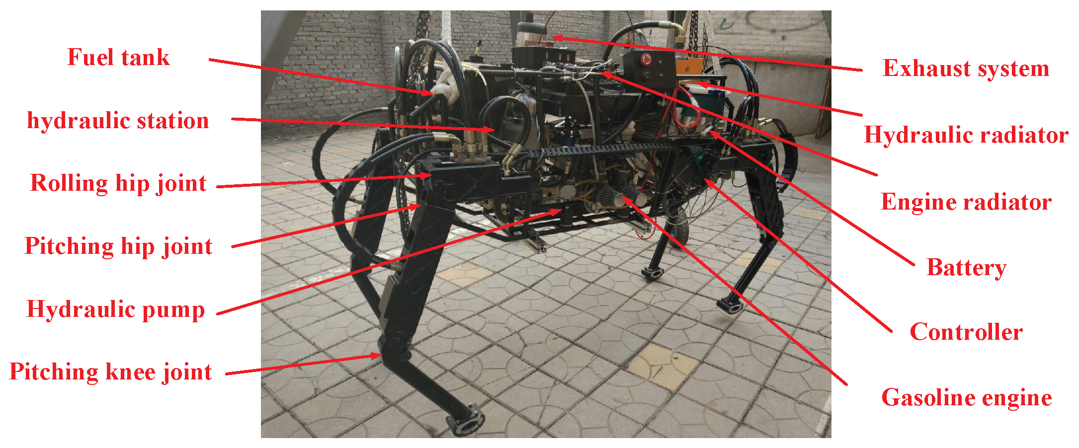
The quadruped robot SCalf was build by the Center for Robotics of Shandong University, as shown in Figure 1. SCalf is a hydraulic actuated robot. The length and width of the robot are 1.4 m and 0.75 m respectively, and the overall weight is 200 kg. The robot consists of a trunk and four legs. The structure of the legs must be designed considering the fact that an improper design can limit the reachable space of the robot legs when operating in the normal quadruped gaits [11]. Therefore, the leg of SCalf is designed as a 3 DOFs (degree of freedom) structure to make the foot endpoint move in a three-dimension workspace with the hip joint as its origin. The three joints of the leg are defined as the rolling hip joint, pitching hip joint, and pitching knee joint. To make the robot easy to control, the SCalf is built symmetrically. The backward/forward configuration is used to improve the gradeability and load capacity.

A variable displacement piston pump is connect to the gasoline engine to provide power for the whole robot system. The onboard hydraulic system and the control system are integrated inside the trunk of the robot. The onboard hydraulic system can distribute a hydraulic flow to the joint actuators and can control the motions of the robot. The robot can be used to transport loads on rough terrains like jungle or mountain, and its load capacity is 200 kg.

To calculate the energy consumption of the robot, the following preconditions are made:

(a) Only the motions in the sagittal plane are studied. The robot is walking on a flat surface with the trot gait.

(b) When walking on a flat surface, the height change of the robot trunk’s center of mass (COM) is ignored.

(c) The trunk of the robot can be regarded as a cuboid, and its COM is assumed to be at the geometric center of the body

2.1. The Kinematics Modelling

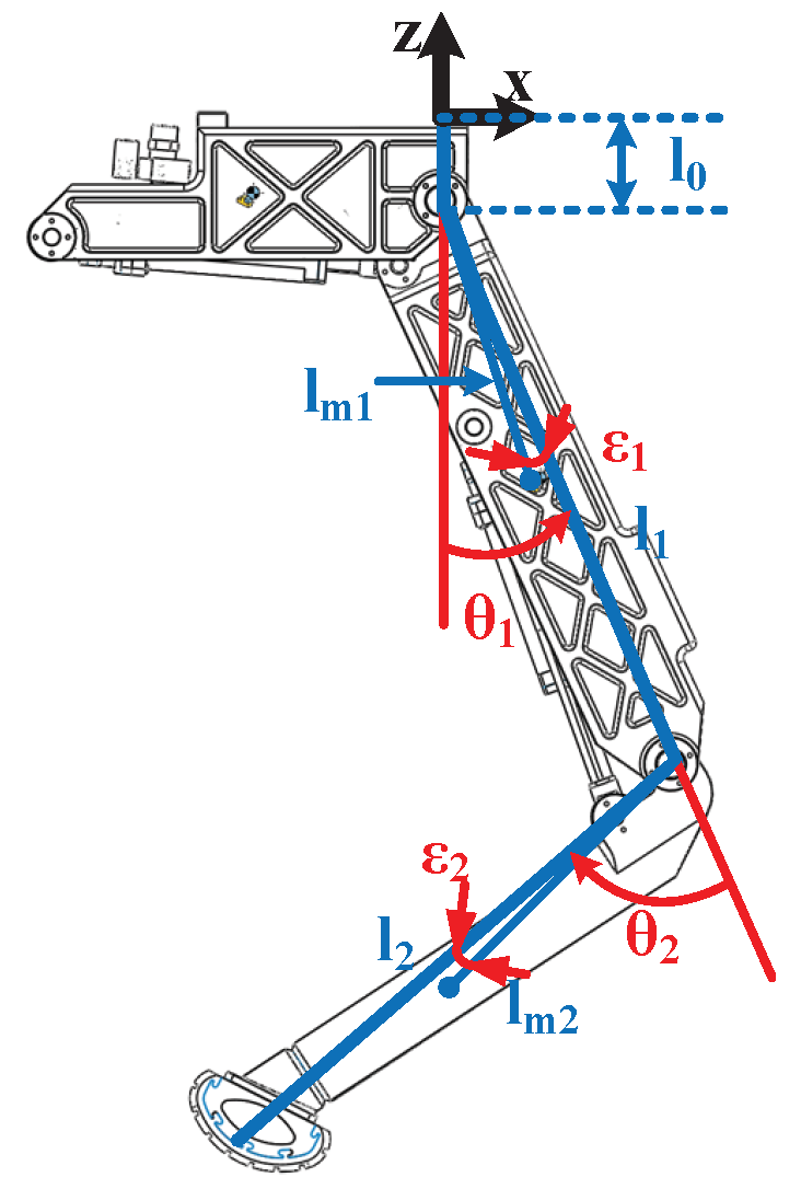
The legs of the robot have the same structure and mechanical parameters. Here, the right front (RF) leg is used as an example. The single leg model is shown in Figure 2. According to precondition (a), the motions of the rolling hip joint are not considered and the rolling hip joint position is set as 0.

In Figure 2, the RF leg can be divided into the hip, thigh, and shank parts. Since the motions of the rolling hip joint are neglected, the hip part can be regarded as the base. The origin of the coordinate frame $\left\{O_h\right\}$ is set at the rolling hip joint. The z-axis direction is vertical to the ground facing upward. The x-axis is pointing to the motion direction of the robot.

The mechanical parameters in Figure 2 are introduced as follows. The lengths of the hip, thigh, and shank parts are $l_0$, $l_1$, and $l_2$ respectively, where $l_0$ = 45 mm. $m_1$ and $m_2$ are the masses of the thigh and the shank parts, respectively. The joint positions of the pitching hip and pitching knee joints are denoted as ${\theta }_1$ and ${\theta }_2$, respectively. The COMs of the thigh and shank parts are defined by $l_{m1}$, $l_{m2}$, ${\epsilon }_1$, and ${\epsilon }_2$. When the thigh and shank parts rotate around their own joint shafts, the moments of inertia are $I_1$ and $I_2$, respectively. The values of these mechanical parameters are listed in

Table 1. The parameters of the thigh and shank parts.

Parameter (i = 1,2)	Thigh	Shank
Mass ($m_i$/Kg)	4.10	2.24
Length ($l_i$/mm)	451.00	405.00
COM position ($l_{mi}$/mm)	210.43	227.20
COM angle (${\epsilon }_i$/rad)	0.037	−0.083
Moment of inertia ($I_i$/Kg·m${}^2$)	0.178	0.057

[12].

Based on the mechanical parameters, the location of the foot endpoint in coordinate frame $\left\{O_h\right\}$ can be written as follows, where ${\theta }_{12}={\theta }_1+{\theta }_2$

$$\left\{\begin{array}{c}x=-l_{2}sin{\theta }_{12}-l_{1}sin{\theta }_1\hfill \\ z=-l_{2}cos{\theta }_{12}-l_{1}cos{\theta }_1-l_0\hfill \end{array}\right.$$

(1)

By solving Equation (1), the joint positions of the RF leg can be obtained as

$$\left\{\begin{array}{c}{\theta }_1=-\varphi -arctan(\frac{x}{-z-l_0})\hfill \\ {\theta }_2=\pi -arccos(\frac{l_1^2+l_2^2-{\xi }^2}{2l_1{l}_2})\hfill \end{array}\right.$$

(2)

where

$$\left\{\begin{array}{c}\xi =\sqrt{{(-z-l_0)}^2+x^2}\hfill \\ \varphi =arccos(\frac{l_1^2+{\xi }^2-l_2^2}{2l_1\xi })\hfill \end{array}\right.$$

(3)

The Jacobian matrix of the single leg model can also be calculated by Equation (1).

$$J=\left[\begin{array}{cc}-l_{1}cos{\theta }_1-l_{2}cos{\theta }_{12}& -l_{2}cos{\theta }_{12}\\ l_{1}sin{\theta }_1+l_{2}sin{\theta }_{12}& l_{2}sin{\theta }_{12}\end{array}\right]$$

(4)

2.2. The Dynamics Modelling

In order to obtain the energy consumptions of the robot, the joint torques must be acquired. The RF leg is used to build the dynamics model of the robot. The standard form of the dynamic equation can be written as Equation (5), where $\mathit{D}(\mathit{\theta })$ is the inertia matrix, $\mathit{H}(\mathit{\theta },\dot{\mathit{\theta }})$ is the Coriolis and centrifugal forces matrix, and $\mathit{G}(\mathit{\theta })$ is the gravitational loading vector.

$${\mathit{\tau }}_{\mathit{J}}=\mathit{D}(\mathit{\theta })\ddot{\mathit{\theta }}+\mathit{H}(\mathit{\theta },\dot{\mathit{\theta }})\dot{\mathit{\theta }}+\mathit{G}(\mathit{\theta })$$

(5)

In the dynamics equation of Equation (5), the inertia matrix $\mathit{D}(\mathit{\theta })$ is a 2 × 2 matrix and can be written as follows:

$$\mathit{D}(\mathit{\theta })=\left[\begin{array}{cc}{D}_{11}(\theta )& D_{12}(\theta )\\ D_{21}(\theta )& D_{22}(\theta )\end{array}\right]$$

(6)

where

$$D_{11}(\theta )=I_1+I_2+m_1{l}_{m1}^2+m_2(l_1^2+l_{m2}^2+2l_1{l}_{m2}cos{\theta }_{\epsilon 2})$$

(7)

$$\begin{array}{c}\hfill D_{12}(\theta )=D_{21}(\theta )=m_2{l}_{m2}^2+m_2{l}_1{l}_{m2}cos{\theta }_{\epsilon 2}+I_2\end{array}$$

(8)

$$D_{22}(\theta )=m_2{l}_{m2}^2+I_2$$

(9)

The Coriolis and centrifugal forces matrix $\mathit{H}(\mathit{\theta },\dot{\mathit{\theta }})$ is shown in Equation (10).

$$\mathit{H}(\mathit{\theta },\dot{\mathit{\theta }})=\left[\begin{array}{cc}{H}_{11}(\theta ,\dot{\theta })& H_{21}(\theta ,\dot{\theta })\\ H_{12}(\theta ,\dot{\theta })& H_{22}(\theta ,\dot{\theta })\end{array}\right]$$

(10)

where

$$H_{11}(\theta ,\dot{\theta })=-\dot{{\theta }_2}{m}_2{l}_1{l}_{m2}sin{\theta }_{\epsilon 2}$$

(11)

$$H_{12}(\theta ,\dot{\theta })=-(\dot{{\theta }_1}+\dot{{\theta }_2})m_2{l}_1{l}_{m2}sin{\theta }_{\epsilon 2}$$

(12)

$$H_{21}(\theta ,\dot{\theta })=\dot{{\theta }_1}{m}_2{l}_1{l}_{m2}sin{\theta }_{\epsilon 2}$$

(13)

$$H_{22}(\theta ,\dot{\theta })=0$$

(14)

The gravitational loading vector $\mathit{G}(\mathit{\theta })$ is

$$\mathit{G}(\mathit{\theta })=\left[\begin{array}{c}{m}_{1}g{l}_{m1}sin{\theta }_{\epsilon 1}+m_{2}g(l_{1}sin{\theta }_1+l_{m2}sin{\theta }_{\epsilon 12})\\ m_{2}g{l}_{m2}cos{\theta }_{\epsilon 12}\end{array}\right]$$

(15)

In the above equations, ${\theta }_{\epsilon 1}={\theta }_1+{\epsilon }_1$, ${\theta }_{\epsilon 2}={\theta }_2+{\epsilon }_2$, and ${\theta }_{\epsilon 12}={\theta }_1+{\theta }_2+{\epsilon }_2$.

Equation (5) shows the situation with no contact between the feet and the ground. When considering the ground reaction force, the dynamics model of the single leg changes to Equation (16), where $F_G$ is the ground reaction force vector. The calculation of $F_G$ will be introduced in the next part.

$$\mathit{\tau }-{\mathit{J}}_{\mathit{G}}^T{\mathit{F}}_{\mathit{G}}=\mathit{D}(\mathit{\theta })\ddot{\mathit{\theta }}+\mathit{H}(\mathit{\theta },\dot{\mathit{\theta }})\dot{\mathit{\theta }}+\mathit{G}(\mathit{\theta })$$

(16)

2.3. The Foot Force Distribution

When analysing the foot force distribution, the slippage between the foot endpoint and the ground is neglected [13]. For the sagittal motions, the lateral forces of the foot endpoints can be ignored, and the ground reaction forces of each leg can be divided into a normal and a tangential component.

The ground reaction force can cause many negative effects like structural damages and control difficulties; therefore, the value of the ground reaction force must be minished. Here, the minimization of norm of the foot force method is used to minimize the norm solution of the foot force and to reduce the compact between the ground and the robot [14].

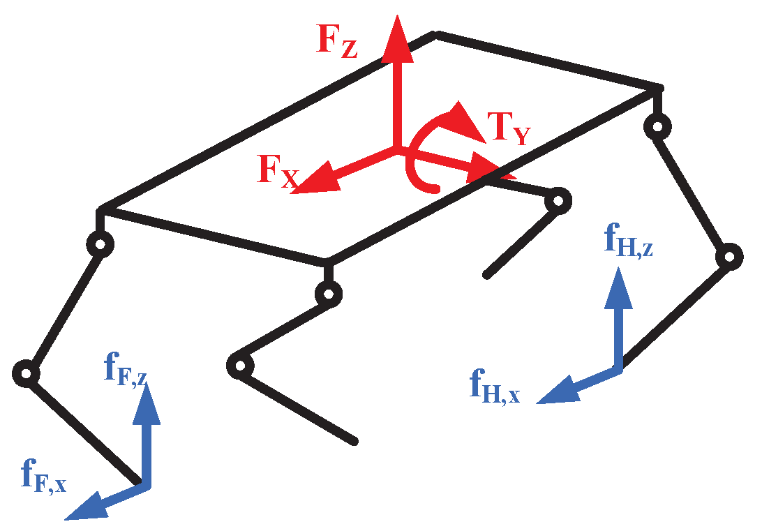
A coordinate frame $\left\{O_b\right\}$ is established at the geometric center of the body. The x axis points to the direction of the motion. The direction of the z axis is vertical to the ground and points upwards. The y axis is defined by the right-hand rule. The static force diagram is illustrated in Figure 3. Here, we assume the RF and LH (left-hind) legs are in the stance phase. ${\mathit{F}}_{\mathit{G}}={[f_{RF},f_{LH}]}^T$ is the ground reaction force vector which contains the ground reaction force of the RF and LH legs, where $f_{RF}={[f_{RF,x},f_{RF,z}]}^T$ and $f_{LH}={[f_{LH,x},f_{LH,z}]}^T$. The vector $\mathit{V}={[F_x,F_z,T_y]}^T$ contains the forces and moment acting on the robot COM in sagittal plane. Under these conditions, the forces and moment balance equations can be written as follows:

$$F_x=f_{RF,x}+f_{LH,x}$$

(17)

$$F_z=f_{RF,z}+f_{LH,z}$$

(18)

$$T_y=f_{RF,x}{z}_{RF}-f_{RF,z}{x}_{RF}+f_{LH,x}{z}_{LH}-f_{LH,z}{x}_{LH}$$

(19)

The Equations (17) to (19) can be written in a matrix form as follows:

$$\mathit{B}·{\mathit{F}}_{\mathit{G}}=\mathit{V}$$

(20)

where

$$\mathit{B}=\left[\begin{array}{cccc}1& 0& 1& 0\\ 0& 1& 0& 1\\ z_{RF}& -x_{RF}& z_{LH}& -x_{LH}\end{array}\right]$$

(21)

In Equation (21), $\{x_{RF},z_{RF}\}$ and $\{x_{LH},z_{LH}\}$ are the coordinates of the support foot endpoints in $\left\{O_b\right\}$.

In Equation (20), there are 4 unknowns but only 3 equations. Here, we use the least squared method to realize the minimization of norm of the foot force method. The result is shown as follows.

$${\mathit{F}}_{\mathit{G}}={\mathit{B}}^T{(\mathit{B}{\mathit{B}}^T)}^{-1}\mathit{V}$$

(22)

In Equation (22), the matrix ${\mathit{B}}^{+}={\mathit{B}}^T{(\mathit{B}{\mathit{B}}^T)}^{-1}$ is also the pseudoinverse matrix of $\mathit{B}$. As the third component of $\mathit{V}$ ($T_y$) is zero, the parameters in the last column of ${\mathit{B}}^{+}$ can be neglected. The value of ${\mathit{B}}^{+}$ is shown as follows.

$${\mathit{B}}^{+}=\left[\begin{array}{ccc}{\displaystyle \frac{b_{11}^{+}}{2\mathsf{\Lambda }}}& {\displaystyle \frac{b_{12}^{+}}{2\mathsf{\Lambda }}}& \times \\ {\displaystyle \frac{b_{21}^{+}}{2\mathsf{\Lambda }}}& {\displaystyle \frac{b_{22}^{+}}{2\mathsf{\Lambda }}}& \times \\ {\displaystyle \frac{b_{31}^{+}}{2\mathsf{\Lambda }}}& {\displaystyle \frac{b_{32}^{+}}{2\mathsf{\Lambda }}}& \times \\ {\displaystyle \frac{b_{41}^{+}}{2\mathsf{\Lambda }}}& {\displaystyle \frac{b_{42}^{+}}{2\mathsf{\Lambda }}}& \times \end{array}\right]$$

(23)

where

$$b_{11}^{+}={(x_{RF}-x_{LH})}^2+2z_{LH}^2-2z_{LH}{z}_{RF}$$

(24)

$$b_{12}^{+}=(x_{RF}+x_{LH})(z_{RF}-z_{LH})$$

(25)

$$b_{21}^{+}=(x_{RF}-x_{LH})(z_{RF}+z_{LH})$$

(26)

$$b_{22}^{+}={(z_{RF}-z_{LH})}^2+2x_{LH}^2-2x_{LH}{x}_{RF}$$

(27)

$$b_{31}^{+}={(x_{RF}-x_{LH})}^2+2z_{RF}^2-2z_{LH}{z}_{RF}$$

(28)

$$b_{32}^{+}=(x_{RF}+x_{LH})(z_{LH}-z_{RF})$$

(29)

$$b_{41}^{+}=(x_{LH}-x_{RF})(z_{RF}+z_{LH})$$

(30)

$$b_{42}^{+}={(z_{RF}-z_{LH})}^2+2x_{RF}^2-2x_{LH}{x}_{RF}$$

(31)

$$\mathsf{\Lambda }={(x_{RF}-x_{LH})}^2+{(z_{RF}-z_{LH})}^2$$

(32)

The Jacobian matrix in Equation (16) can be written as follows:

$${\mathit{J}}_{\mathit{G}}=\left[\begin{array}{cc}{\mathit{J}}_{\mathit{F}}& \mathbf{0}\\ \mathbf{0}& {\mathit{J}}_{\mathit{H}}\end{array}\right]$$

(33)

In Equation (33), ${\mathit{J}}_{\mathit{F}}$ and ${\mathit{J}}_{\mathit{H}}$ are the Jacobian of the RF and LH legs respectively.

3. The Energy Analysis of The Scalf

3.1. Energy Model

In order to analyze the energy consumption conditions of SCalf, the energy model must be established. For SCalf, the calculation of the energy consumption is obtained by the integration of the joint power. The joint power consists of the mechanical power and heat rate, as shown in Equation (34), where T is the gait cycle, E is the energy consumption in one gait cycle, and P is the joint power.

$$\begin{array}{cc}\hfill E& ={\int }_0^{T}Pdt\hfill \\ & ={\int }_0^T(|\tau \dot{\theta }|+f_f{\dot{x}}_p)dt\hfill \end{array}$$

(34)

In the second line of Equation (34), $f_f$ and ${\dot{x}}_p$ are the friction and piston velocity of the hydraulic cylinder, respectively. The joint torque $\tau$ can be acquired by the dynamics analysis.

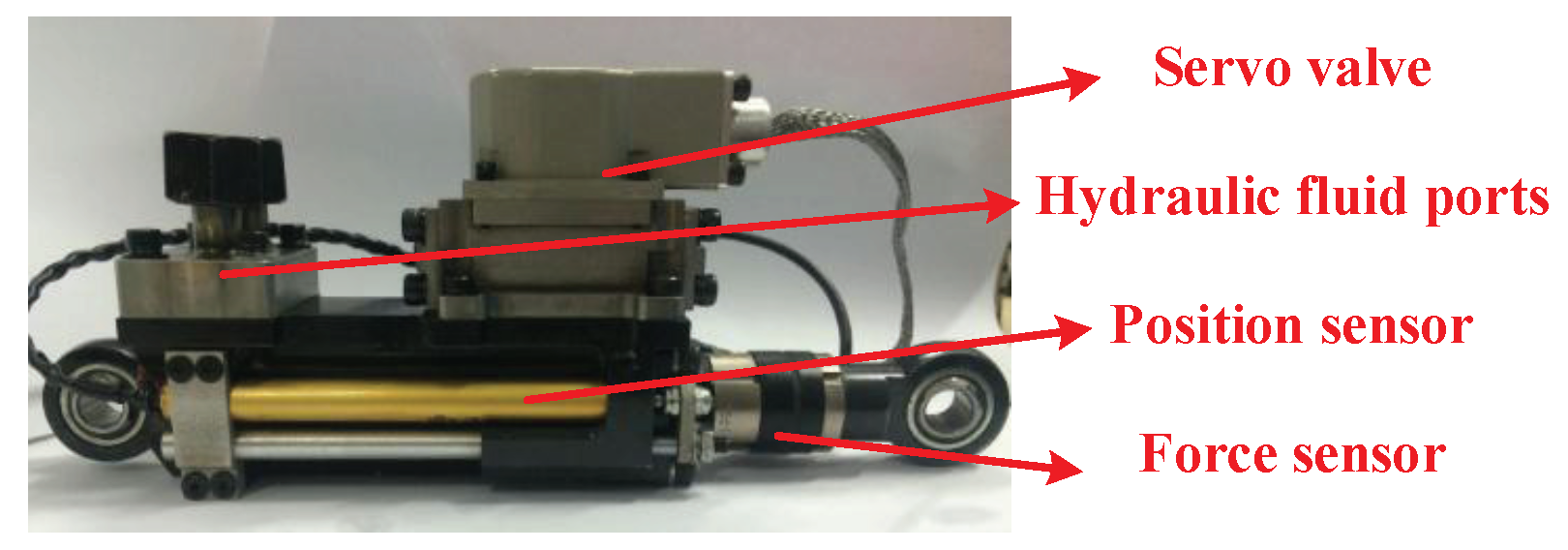
The structure of the hydraulic actuator is shown in Figure 4. The displacement and force of the piston can be measured by the position and force sensors. The motions of the piston are controlled by the servo valve.

The friction of hydraulic cylinders are strongly coupled by many parameters, and it has a high nonlinearity. It depends on many conditions like the cylinder velocity ${\dot{x}}_p$, the pressure difference $\Delta p$ across the piston and possibly on the cylinder position $x_p$, and the temperature t [15]. The SCalf uses the asymmetry cylinders to realize the joint motions. The model parameters are different when the actuator are extending or shorting. According to the research made by Nissing, the model of the hydraulic frictions can be written in Equation (35) [16].

$$f_f({\dot{x}}_p)=\left\{\begin{array}{c}{B}^{+}{\dot{x}}_p+\left(F_{c0}^{+}+F_{s0}^{+}{e}^{-\frac{|{\dot{x}}_p|}{C_s^{+}}}\right),{\dot{x}}_p>0\hfill \\ B^{-}{\dot{x}}_p-\left(F_{c0}^{-}+F_{s0}^{-}{e}^{-\frac{|{\dot{x}}_p|}{C_s^{-}}}\right),{\dot{x}}_p<0\hfill \end{array}\right.$$

(35)

In Equation (35), B is the viscous friction coefficient (Ns/m), $F_{c0}$ is the Coulomb friction coefficient (N), $F_{s0}$ is the static friction coefficient (N), and $C_S$ is the attenuation coefficient of static friction. Using the measured result made by Polzer et al. [17], the parameters in Equation (35) can be obtained as follows. When ${\dot{x}}_p\ge$ 0, B = 220 Ns/m, $F_{c0}$ = 50 N, $F_{s0}$ = 30 N and $C_s$ = 0.015 m/s. When ${\dot{x}}_p<$ 0, B = 180 Ns/m, $F_{c0}$ = 50 N, $F_{s0}$ = 20 N, and $C_s$ = 0.007 m/s.

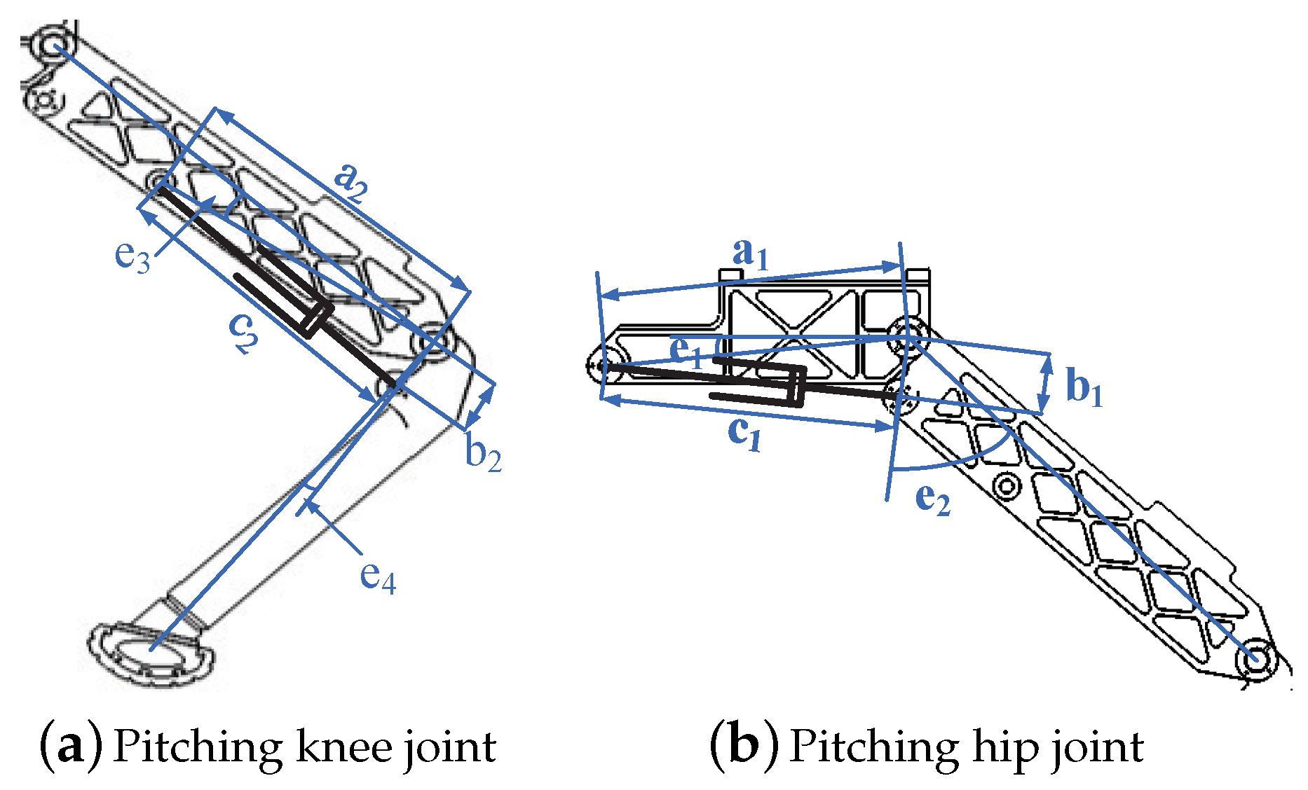
The cylinder velocities can be obtained by the differential of cylinder lengths. The cylinder lengths can be calculated by the mechanical parameters in Figure 5 and

Table 2. The mechanical parameters used in Figure 5.

Joint	${\mathit{a}}_{\mathit{i}}$ (mm)	${\mathit{b}}_{\mathit{i}}$ (mm)	Angles (°)
Pitching hip joint	289.26	56.87	$e_1$ = 0.094	$e_2$ = 0.96
Pitching knee joint	289.26	56.89	$e_3$ = 0.14	$e_4$ = 0.041

.

The relationship between the cylinder lengths and mechanical parameters are shown in Equation (36)

$$\left\{\begin{array}{c}{c}_1=\sqrt{a_1^2+b_1^2-2a_1{b}_{1}cos(-{\theta }_1+\frac{\pi }{2}-e_1-e_2)}\hfill \\ c_2=\sqrt{a_2^2+b_2^2-2a_2{b}_{2}cos(-{\theta }_2+\pi -e_3+e_4)}\hfill \end{array}\right.$$

(36)

3.2. Energetic Criterion

In order to evaluate the energy consumptions of robot motions, the corresponding energetic criterion should be designed.

In this paper, a criterion called energy cost is considered. The energy cost $E_{cost}$ is defined as the energy consumption for a unit distance. It represents the energy consumption of the robot movements intuitively. It is defined by assuming that the negative work produced by the actuators are dissipated.

$$E_{cost}=\frac{1}{x(T)-x(0)}{\int }_0^{T}Pdt[J/m]$$

(37)

4. The Foot Trajectory Analysis

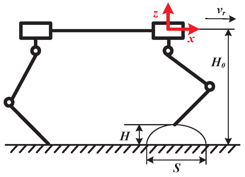
The SCalf team has already done some research on the gait trajectory planning [18,19,20], but they only considered the situations under the duty cycle as 50%. In this paper, a more general trot gait trajectory is proposed. In the trot gait, S is the step length, T is the gait cycle, H is the step height, and $H_0$ is the standing height, as illustrated in Figure 6. $\beta$ is the duty cycle of the trot gait. The velocity of the robot $v_r$ can be obtained by the step length S and the gait cycle T by using Equation (38).

$$v_r=2S/T$$

(38)

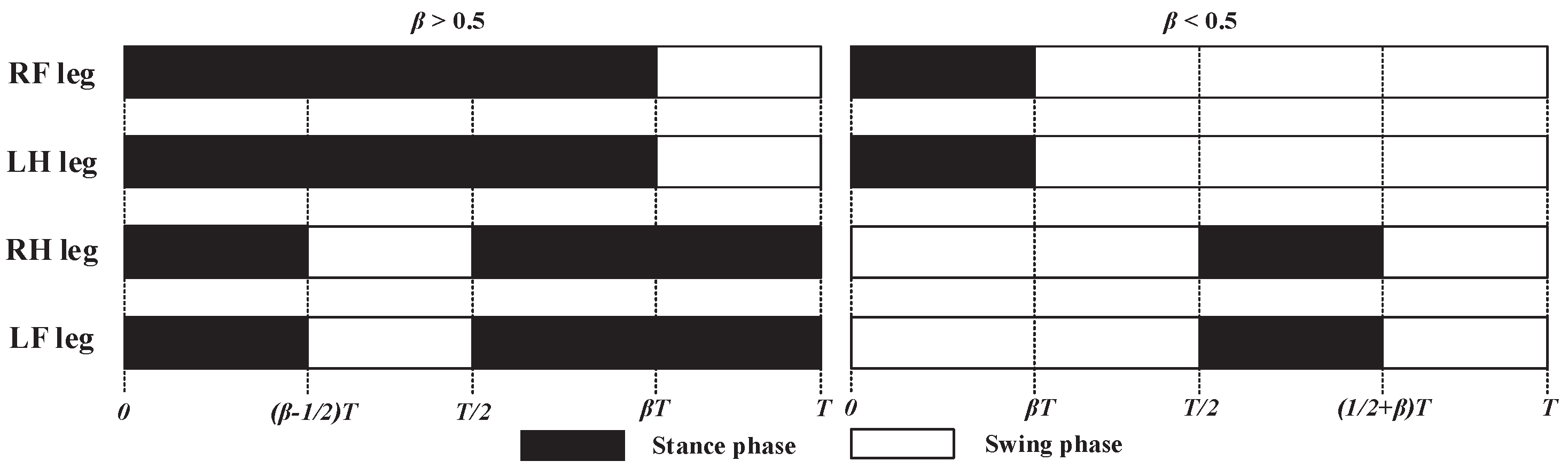
During the movements of the robot, the legs will swing periodically with respect to the trunk. In order to make the quadruped robot walk at a steady speed, this work realizes the trajectory planning of the robot by simulating the trajectory of the quadruped animals’ feet. Based on the motions of the horses, a foot trajectory including the cubic spline interpolation curve and the straight line is studied. The phases of the four legs are shown in Figure 7, where the two feet on the diagonal have the same movements.

Here, the trajectory of the RF leg is analyzed. During the stance phase, the trunk of the robot is moving forward. According to Equations (16), (22), and (34), in order to minimize the energy consumption, joint torques have to be as small as possible. Then, the first component of M, which is $F_x=Ma$, have to be small. Therefore, the trunk acceleration a is set as zero, and the motions of the stance phase become uniform motions in the x direction. The positions in the z direction are equal to −$H_0$. The trajectory equation of the stance phase in the coordinate frame $\left\{O_b\right\}$ can be obtained in Equation (39).

$$\begin{array}{c}\hfill \left\{\begin{array}{c}x(t)=\frac{S}{2}(1-\frac{2t}{\beta T})\hfill \\ z(t)=-H_0\hfill \end{array}\right.\end{array},0<t\le \beta T$$

(39)

In order to obtain the parameters of the foot trajectory during the swing phase, the initial and terminated conditions of the stance phase are listed in

Table 3. The initial and terminated conditions of the stance phase.

Items (time)	x Direction	z Direction
position (0)	${\displaystyle \frac{S}{2}}$	$H_0$
position ($\beta T$)	$-{\displaystyle \frac{S}{2}}$	$H_0$
velocity (0)	$-{\displaystyle \frac{S}{\beta T}}$	0
velocity ($\beta T$)	$-{\displaystyle \frac{S}{\beta T}}$	0

, including the positions and velocities of the foot endpoint in the x and z directions.

In the swing phase, the cubic spline interpolation and the cosine curve are used in the x and z directions respectively. In the trajectory expression of the x direction, the coefficients of the cubic equation are obtained from the data in Table 3. For the cosine curve in the z direction, the foot endpoint reaches the curve’s top in the middle of the swing phase. According to the above conditions, the foot trajectory can be written in Equation (40).

$$\begin{array}{c}\hfill \left\{\begin{array}{c}x(t)=\frac{S}{2}(a_3{t}^3+a_2{t}^2+a_{1}t+a_0)\hfill \\ z(t)=-H_0+\frac{H}{2}\left\{1-cos\left[\frac{2\pi t}{(1-\beta T)}-\frac{2\pi \beta }{(1-\beta )}\right]\right\}\hfill \end{array}\right.\end{array},\beta T<t\le T$$

(40)

where

$$\left\{\begin{array}{c}\gamma ={(\beta -1)}^3\hfill \\ a_0=\frac{({\beta }^3-{\beta }^2-3\beta -1)}{\gamma }\hfill \\ a_1=\frac{-2({\beta }^3-3{\beta }^2-3\beta -1)}{\gamma \beta T}\hfill \\ a_2=\frac{-6(\beta +1)}{\gamma \beta T^2}\hfill \\ a_3=\frac{4}{\gamma \beta T^3}\hfill \end{array}\right.$$

(41)

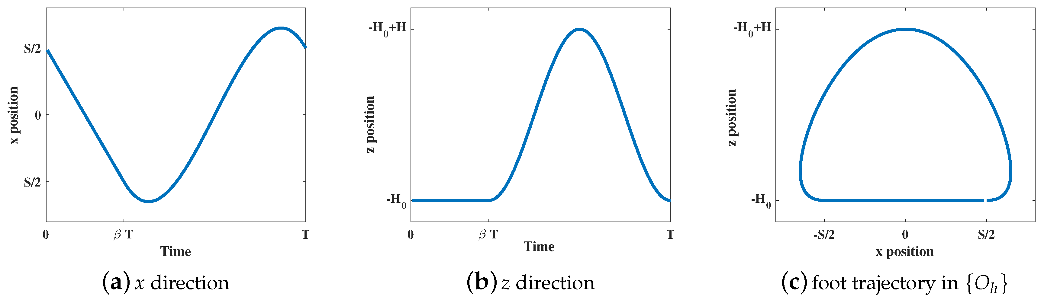
The curves of the foot trajectory are shown in Figure 8, including the curves of the x direction, of the z direction, and in coordinate frame $\left\{O_h\right\}$. Here, the gait parameters are chosen as follow: S = 0.25 m, T = 0.5 s, H = 0.08 m, $H_0$ = 0.5 m, and $\beta$ = 0.3.

The advantages of this foot trajectory are listed as follows:

(a) When gait phases switch, the velocities of the foot endpoint are zero, which can eliminate the collisions between the foot and the ground.

(b) The trunk velocity and the velocity of the swing leg are changing with no mutation.

(c) At the beginning and end of the swing phases, the foot endpoint will move back some distance, which can improve the ability of the robot to move over obstacles and to adapt to certain undulating grounds.

5. Simulations

In this section, we will study the influences of different gait parameters on the energy consumptions. The four legs of the SCalf have the same structure and mechanical parameters; therefore, the energy consumption of the RF leg can be regarded as a quarter of the total energy consumption.

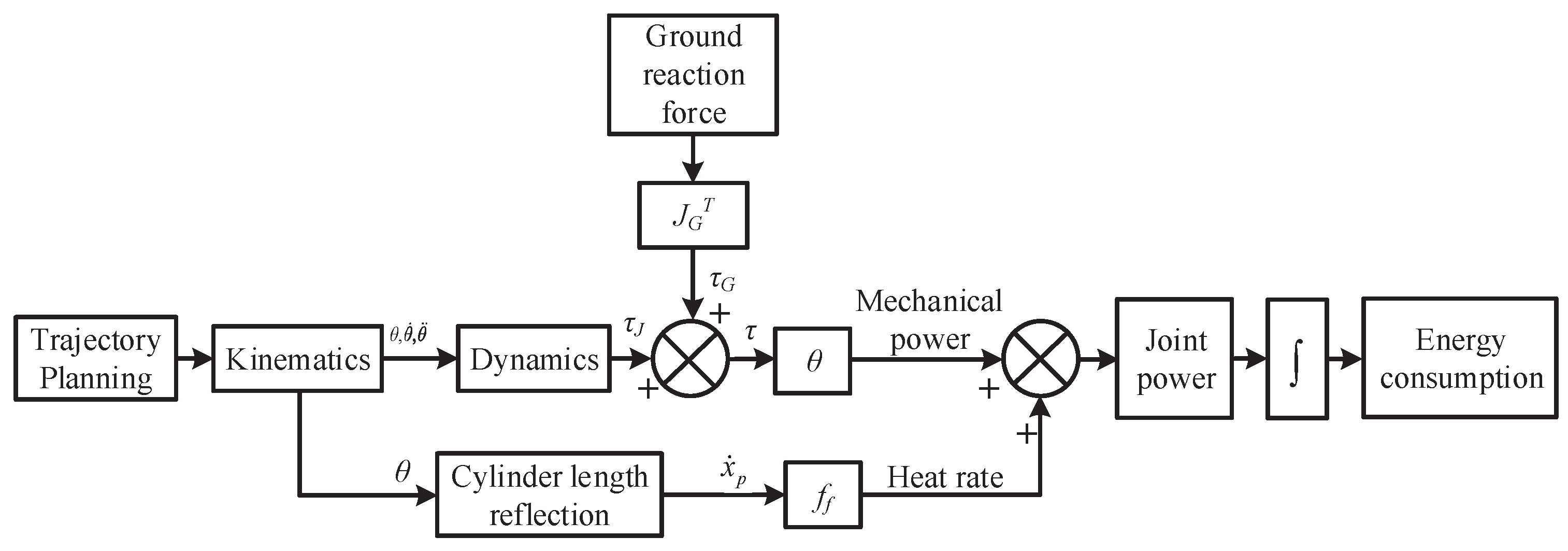
A set of experiments are implementing in MATLAB. The total energy consumptions as well as the energy consumptions during the stance and swing phases using different gait parameters are calculated, and the energetic criterion is used to evaluate the robot motions. The flow chart of the simulation is illustrated in Figure 9.

In the simulations, the robot trunk can be regarded as a cuboid, and the mass of trunk is M = 200 kg. The distances between the origins of $\left\{O_b\right\}$ and $\left\{O_h\right\}$ in the x and z directions are 0.68 m and 0.15 m respectively, which are used to confirm the position of the foot endpoints in $\left\{O_b\right\}$.

Different gait parameters such as step length S, gait cycle T, step height H, standing height $H_0$, and duty cycle $\beta$ are studied in this section. The default values of the gait parameters are listed in

Table 4. The default values of the gait parameters.

Gait Parameter	Default Value
step length S	0.25 m
gait cycle T	0.5 s
step height H	0.08 m
standing height $H_0$	0.6 m
gait cycle $\beta$	0.5

. Under the default condition, the velocity of the robot is 1 m/s.

5.1. Validation of the Energy Model

In order to verify the energy model proposed in this paper, some experiments are carried out. Different from the electrical actuated robots [21,22], the energy consumption of a hydraulic actuated robot is obtained by the data of joint sensors. For SCalf, the position and force sensors mounted on the actuator (Figure 4) are used to measure the cylinder lengths $c_i$ and joint forces ${\tau }_i$ (i = 1, 2). Here, the equations of the RF leg are used. The mechanical parameters can be found in Table 2.

The joint angular velocities in Equation (34) can be obtained by the following equations.

$$\begin{array}{c}\hfill \left\{\begin{array}{c}{\theta }_1=\frac{\pi }{2}-arccos(\frac{a_1^2+b_1^2-c_1^2}{2a_1{b}_1})-e_1-e_2\hfill \\ {\theta }_2=\pi -arccos(\frac{a_2^2+b_2^2-c_2^2}{2a_2{b}_2})-e_3+e_4\hfill \end{array}\right.\end{array}$$

(42)

$$\dot{{\theta }_i}=\frac{d\theta }{dt},i=1,2$$

(43)

The torques in Equation (34) are equal to the forces multiplied by their force arms, where i = 1, 2.

$${\tau }_i=f_i·a_i\sqrt{1-cos(\frac{a_i^2+c_i^2-b_1^2}{2a_i{c}_i})}$$

(44)

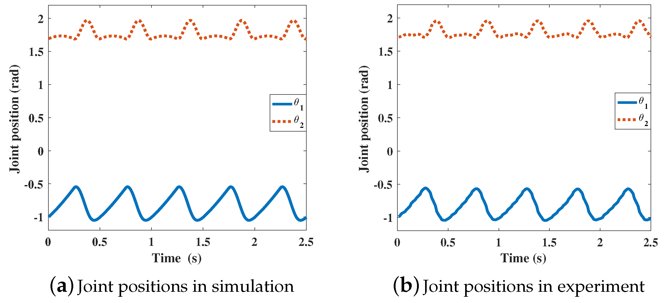
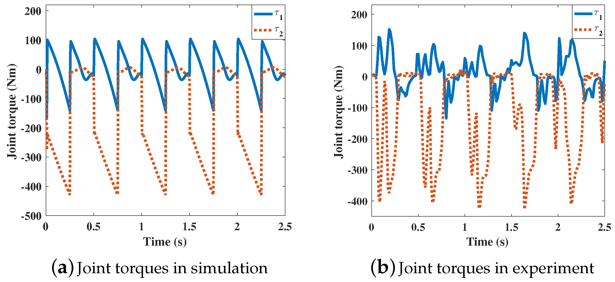
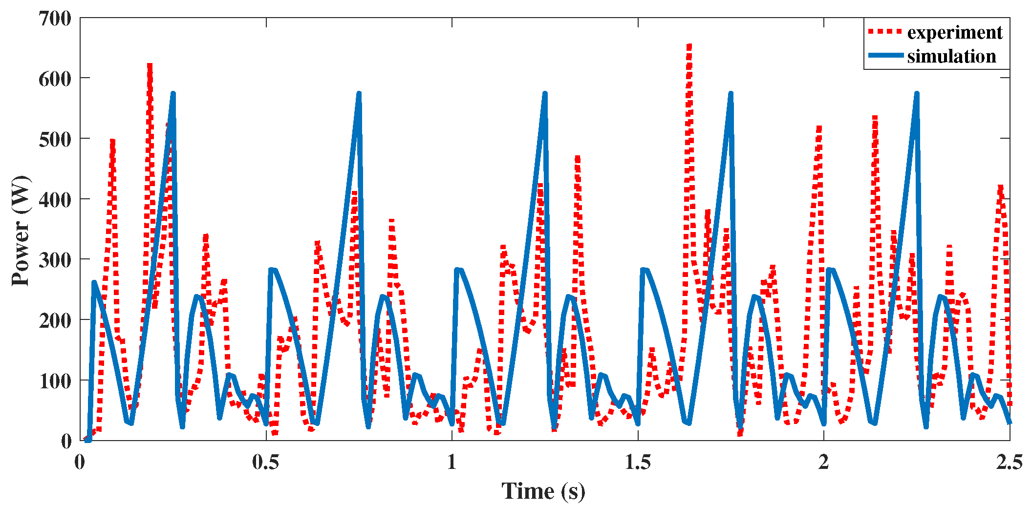
In the experiment, the gait parameters are chosen from Table 4. The sensor data are recorded with a frequency of 80 Hz. In this work, data of 5 gait cycles are recorded. The curves of joint positions, joint torques, and the leg power of the RF leg are illustrated in Figure 10, Figure 11 and Figure 12.

From the above experiment results, the joint positions, joint torque, and leg power have the same trends in the experiment and simulation. The energy consumptions during 5 cycles are 393.69 J and 421.80 J for the experiment and simulation, respectively. The mean powers of the RF leg in the experiment and simulation can be calculated as 157.48 W and 168.72 W respectively. The differences between the data are mainly caused by the foot force distribution. Based on the energy consumptions and average power, the proposed energy model is verified.

5.2. Simulation Results

5.2.1. Step Length

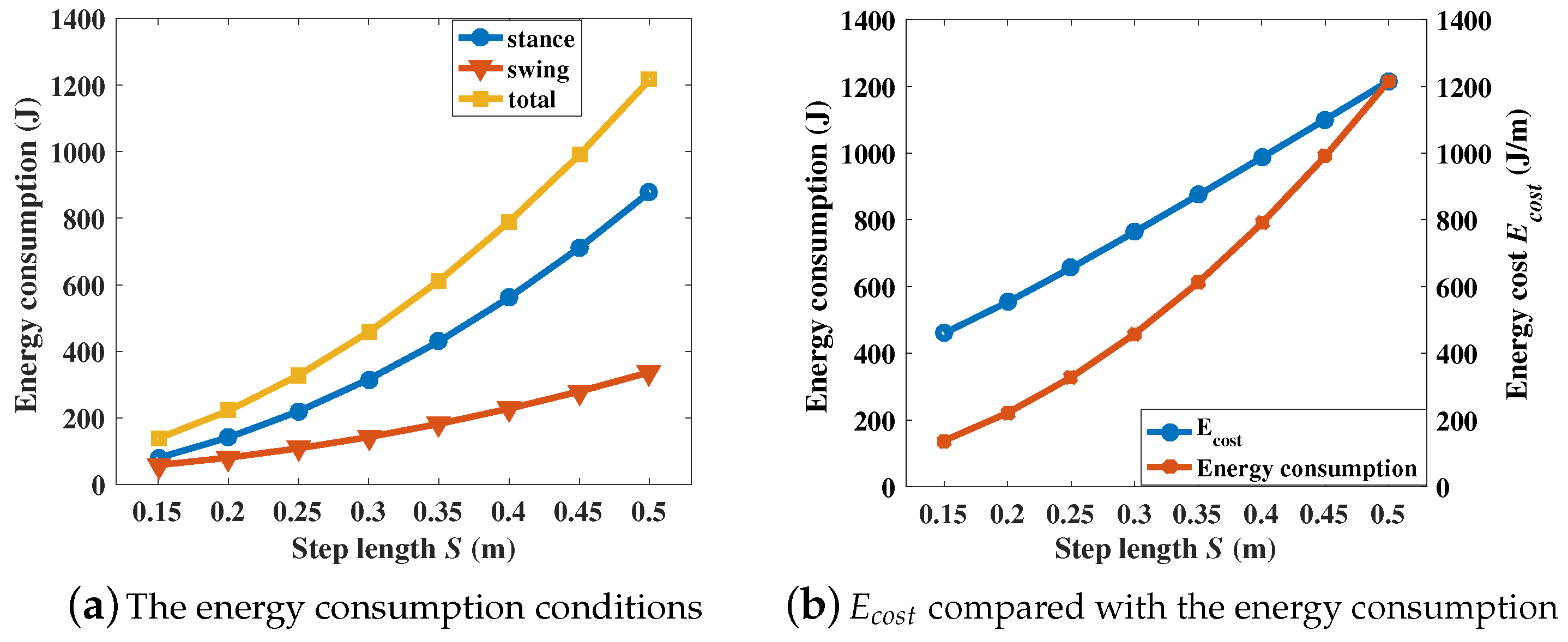
In this part, the step lengths are set as different values while the other gait parameters use default values. The step lengths ranges from 0.15 m to 0.5 m with an interval of 0.05 m. The energy consumption conditions and the $E_{cost}$ are shown in Figure 13.

From Figure 13, we can know that with the increasement of the step length, the energy consumption during different phases and $E_{cost}$ are both increasing but that the growth rate of $E_{cost}$ is slower than the energy consumption.

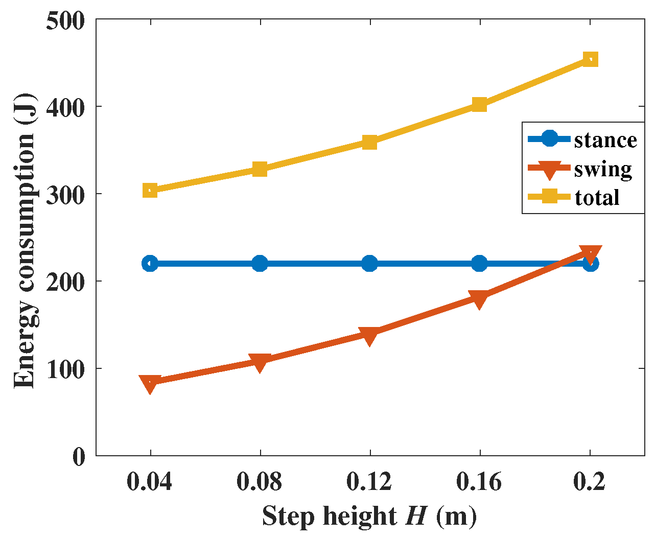
5.2.2. Step Height

The energy consumption conditions with different step height are shown in Figure 14 and

Table 5. $E_{cost}$ with different step heights.

step height (m)	0.04	0.08	0.12	0.16	0.20
$E_{cost}$ (J/m)	607.44	656.17	719.80	803.52	907.08

. The step heights H are chosen as 0.04, 0.08, 0.12, 0.16, and 0.20 m. According to Equation (37), when the step length S is set as a constant, the energy consumption is proportional to $E_{cost}$.

Based on the equations of the foot trajectory, the step height has no influence on the stance phase, which can be verified in Figure 14. With the augmentation of the step height, the movement distance of the leg endpoint as well as the joint energy consumptions will increase. Considering the obstacle crossing ability of the robot, a proper value of the step height needs to be chosen.

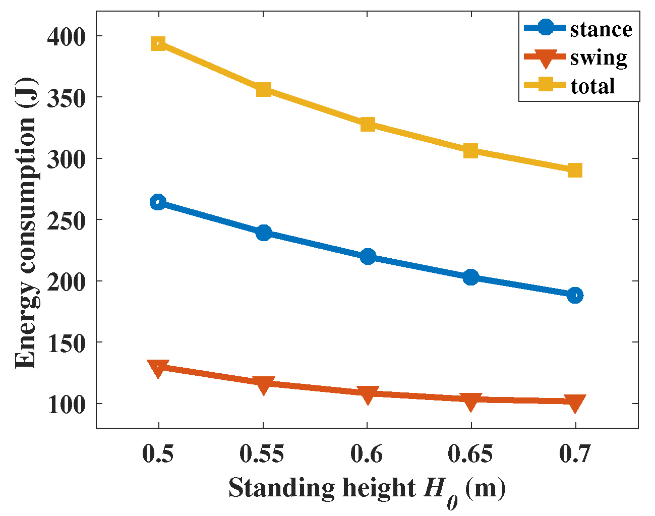
5.2.3. Standing Height

Considering the mechanical limitation and the ranges of the joint position, the standing heights $H_0$ are chosen between 0.5 to 0.7 m with a step of 0.05 m. The values of $E_{cost}$ are proportional to the energy consumptions.

The results are illustrated in Figure 15 and

Table 6. $E_{cost}$ with different standing heights.

standing height (m)	0.5	0.55	0.6	0.65	0.7
$E_{cost}$ (J/m)	787.17	712.88	656.17	612.50	580.59

. When the distance between the trunk and the ground is small, the joints have to sustain more weight, which will increase the joint torques, and the energy consumption will increase. However, if the distance between the trunk and the ground is too large, the COM of the robot will rise, which will reduce the movement stability of the robot.

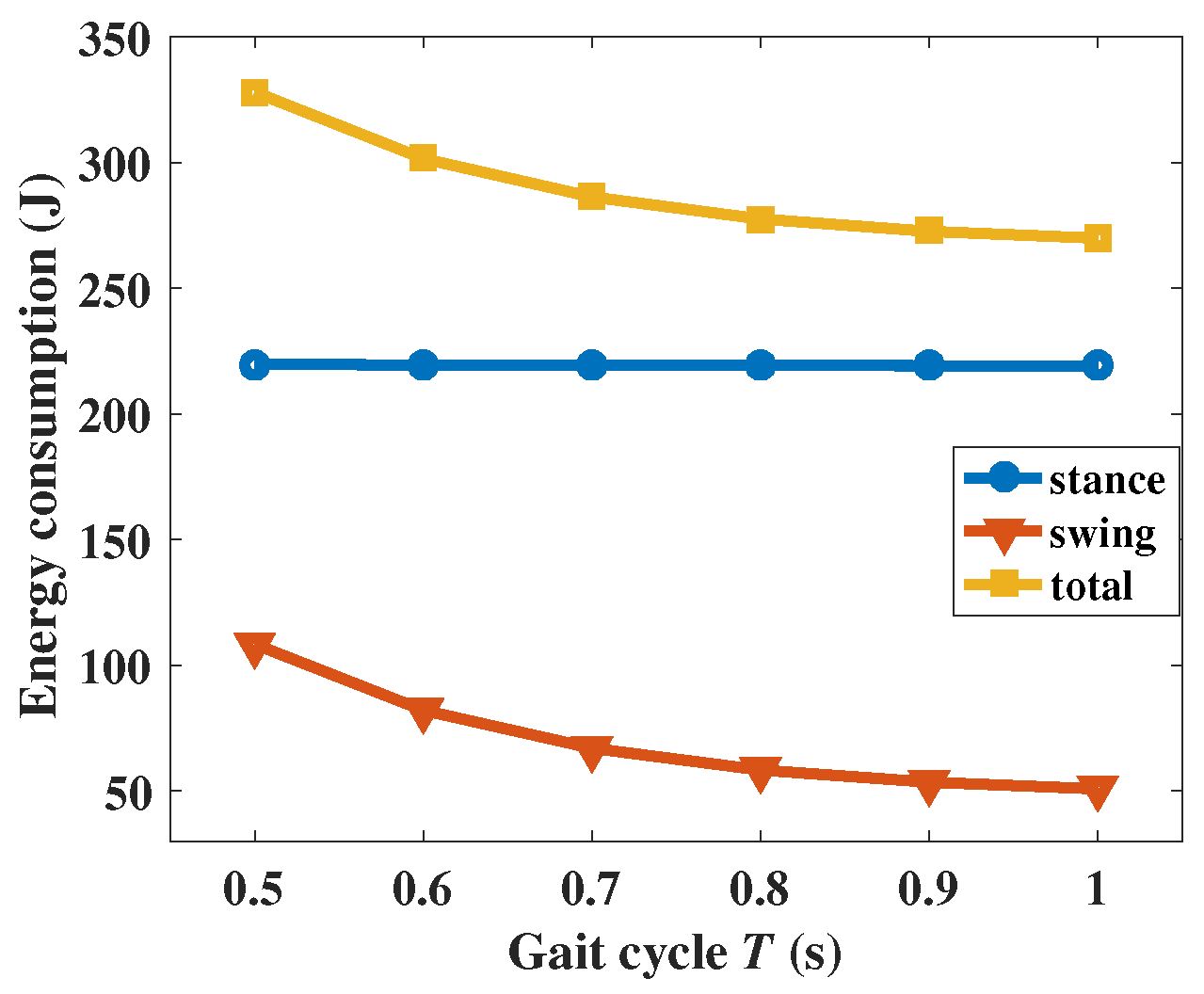
5.2.4. Gait Cycle

The gait cycle is the reciprocal of the gait frequency (f). Here, we choose the gait cycles as 0.5, 0.6, 0.7, 0.8, 0.9, and 1.0 s to calculate the energy consumption. The results are listed in Figure 16 and

Table 7. $E_{cost}$ with different gait cycles.

gait cycle (s)	0.5	0.6	0.7	0.8	0.9	1.0
$E_{cost}$ (J/m)	656.17	603.20	572.72	555.15	545.33	539.83

.

With a large gait cycle, the velocity and acceleration of the joint angle will be decreased and the joint torque can be reduced according to Equation (5). From Figure 16, we can know that the energy consumption in the swing phase will decrease with the augmentation of the gait cycle but that the energy consumptions during the stance phase remain the same. For the motion of the SCalf, a gait with a large cycle can reduce the energy consumption but will make the motion unstable.

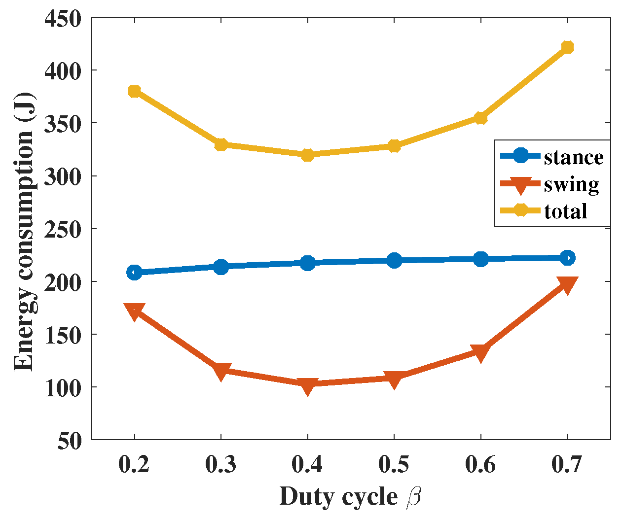
5.2.5. Duty Cycle

When the duty cycle is less or greater than 0.5, there will be conditions like a four-foot touchdown or a four-foot flight. The energy consumptions with different duty cycles are shown in Figure 17, and the $E_{cost}$ are listed in

Table 8. $E_{cost}$ with different duty cycles.

duty cycle	0.2	0.3	0.4	0.5	0.6	0.7
$E_{cost}$ (J/m)	761.00	659.62	639.68	656.17	710.71	842.25

.

For different duty cycles, the different energy costs $E_{cost}$ are proportional to the energy consumptions, too. From Figure 17, we can know that the energy consumptions during the stance phases are nearly the same. When the duty cycle is large or small, the energy consumption during the swing phase will grow rapidly. The optimal duty cycle falls into the range of 0.3 to 0.5.

5.3. Discussion

In robot motions, the velocity of the robot is an important comprehensive index. According to Equation (38), the robot velocity is decided by the step length S and gait cycle T; both big S or short T can increase robot velocity. Based on the results in Figure 13 and Figure 16, big S and short T will both increase the energy consumption. When choosing the values of S and T, the mechanical limitations and control stability should be considered. We notice that the growth rate of the energy consumption caused by S is higher than that caused by T. Therefore, when the robot velocity is determined, a gait with a small step length and a short gait cycle should be chosen.

For the step height H and standing height $H_0$, there are conflicts between low energy consumption and control effectiveness. Therefore, the selection of these parameters should consider the actual terrain and control situation.

Most researchers only study foot trajectories with the duty cycle as 50%. From the results in Figure 17, we can know that the optimal duty cycle falls into the range of 0.3–0.5, which would make the common trot gait become a flying trot gait.

According to the above discussions, for a typical situation with the robot velocity as 1 m/s, the gait parameters are chosen as follows: step length S = 0.25 m, gait cycle T = 0.5 s, step height H = 0.08 m, standing height $H_0$ = 0.6 m, and gait cycle $\beta$ = 0.4. The energy consumptions under these gait parameters can be calculated as 217.45 J, 102.39 J, and 319.84 J for the stance phase, swing phase, and total consumption. The energy cost of this condition is 639.68 J/m.

6. Conclusions

In this work, the energy consumption conditions of the quadruped robot SCalf are studied. The kinematics model of the robot was studied, and the dynamics model was established based on the foot force distribution analysis. A complete energy model including the mechanical power and heat rate was derived. In order to describe the motions of the robot, a universal foot trajectory based on cubic spline interpolation is proposed. Different gait parameters including step length, gait cycle, step height, standing height, and duty cycle are considered in the trajectory. After obtaining the equations of the foot trajectory, the influences of different gait parameters on energy consumption are studied through a simulation. According to the results of the simulation, during the motion, a trot gait with a short step length and a small gait cycle should be chosen. The obstacle crossing ability and motion stability need to be considered in the selection of the standing height and step height. The duty cycle of the gait should be selected in the range of 0.3 to 0.5. For a typical situation with the robot velocity as 1 m/s, the gait parameters are chosen as follows: step length S = 0.25 m, gait cycle T = 0.5 s, step height H = 0.08 m, standing height $H_0$ = 0.6 m, and gait cycle $\beta$ = 0.4.