Parametrical Non-Complex Tests to Evaluate Partial Decentralized Linear-Output Feedback Control Stabilization Conditions from Their Centralized Stabilization Counterparts

Abstract

This paper formulates sufficiency-type linear-output feedback decentralized closed-loop stabilization conditions if the continuous-time linear dynamic system can be stabilized under linear output-feedback centralized stabilization. The provided tests are simple to evaluate, while they are based on the quantification of the sufficiently smallness of the parametrical error norms between the control, output, interconnection and open-loop system dynamics matrices and the corresponding control gains in the decentralized case related to the centralized counterpart. The tolerance amounts of the various parametrical matrix errors are described by the maximum allowed tolerance upper-bound of a small positive real parameter that upper-bounds the various parametrical error norms. Such a tolerance is quantified by considering the first or second powers of such a small parameter. The results are seen to be directly extendable to quantify the allowed parametrical errors that guarantee the closed-loop linear output-feedback stabilization of a current system related to its nominal counterpart. Furthermore, several simulated examples are also discussed.

1. Introduction

Control systems are very important in real world applications and, therefore, they have been investigated exhaustively concerning their properties of stability, stabilization, controllability control strategies etc. See, for instance, [1,2,3,4] and references therein. Some extra constraints inherent to some systems, like solution positivity in the case of biological systems or human migrations or the needed behavior robustness against parametrical changes of disturbance actions add additional complexity to the related investigations and need the use of additional mathematical or engineering tools for the research development, [5,6,7]. A large variety of modeling and design tools have to be invoked and developed in the analysis depending on the concrete systems under study and their potential applications as, for instance, the presence of internal and external delays, discretization, dynamics modeling based on fractional calculus, the existence of complex systems with interconnected subsystems, [8,9,10,11,12,13], hybrid coupled continuous/digital tandems, nonlinear systems and optimization and estimation techniques [14,15,16,17,18,19] as well as robotic and fuzzy-logic based systems, [20,21]. In particular, decentralized control is a useful tool for controlling dynamic systems by cutting some links between the dynamics coupling a set of subsystems integrated in the whole system at hand. It is claimed to keep the main properties related to the use of centralized control such as stability, controllability, observability, etc. In summary, a centralized controller keeps all the information on the system and coupling links as available to the control designer while decentralized control ignores some of such information or even cuts on occasions some of coupling signals between the various subsystems integrated in the whole system at hand. It can be pointed out that the stability studies are often performed trough Lyapunov theory which requires to find a Lyapunov function (see [20,21] and some references therein). It turns out that, if the neglected couplings are strong and are not taken into account by the controller, the stabilization and other properties such as the controllability can become lost. The use of decentralized stabilization and control tools is of interest when the whole system has physically separated subsystems that require the implementation of local control actuators but the control has to be global for the whole system. An ad-hoc example provided in [2,3,4,19] where decentralized control is of a great design interest is the case of several coupled cascade hydroelectric power plants allocated in the same river but separated far away from each other. It has to be pointed out that the term “decentralized control” versus “centralized control” refers to the eventual cut of links of the shared information between tandems of integrated subsystems, or coupling signals between them, to be controlled rather than to the physical disposal of the controller. In other words, if the whole controller keeps and uses all the information on measurable outputs and control components design to implement the control law, such a control is considered to have a centralized nature even if its various sub-control stations are not jointly allocated. It is a common designer´s basic idea in mind for complex control designs to try to minimize the modeling designs and computational loads without significantly losing the system´s performance and its essential properties. For instance, in [8], the dynamic characteristic of a discrete-time system is given as an extended state space description in which state variables and output tracking error are integrated while they are regulated independently. The proposed robust model predictive control is much simpler than the traditional versions since the information of the upper and lower bounds of the time-varying delay are used for design purposes. On the other hand, in [9], a control law might be synthesized for a hydropower plant with six generation units working in an alternation scheme. To assess the behavior of the controlled system, a model of such a nonlinear plant is controlled by a fractional proportional/integral/derivative control device through a linearization of its set points, the fractional part being relevant in the approach on the controller derivative actions. In addition, a set of applied complex control problems are studied, for instance, in [10,11,12,13,14,15,16] with the aim of giving different ad hoc simplification tools to deal with the appropriate control methodologies. In particular, a decentralized control approach is proposed in [16].

In this paper, the decentralized control design versus its decentralized control counterpart, under eventual output linear feedback, are studied from the point of view of the amount of information that can be lost or omitted in terms of the total or partial knowledge of the coupled dynamics between subsystems necessary in the decentralized case to keep the closed-loop stability. The study is made by using the information on the worst-case deviation, in terms of norms, between the respective matrices of open-loop dynamics and the respective controller gains under which the closed-loop stability is kept. This paper is organized as follows. The problem statement is given in Section 2 while the main stabilization results of the paper are provided in Section 3. The proofs of some of the results of Section 3, which are technically involved, but conceptually simple, are distributed in various technical auxiliary that are given in Appendix A and Appendix B. It is claimed to give a non-complex method to test the feasibility of the implementation of decentralized control and conditions for its design, which be a fast and simpler stability test compared to Lyapunov stability theory [20,21], for instance, under a partial removal of information or physical cuts of links of coupling dynamics between the various subsystems or state, control and output components. Section 4 discusses several examples and, finally, the concluding remarks end the paper.

Notation

$$\overline{n}=\left\{1,2,\cdots \hspace{0.17em},\hspace{0.17em}n\right\},$$

$${\mathit{R}}_{+}=\left\{\hspace{0.17em}z\in \mathit{R}\hspace{0.17em}:z>0\right\} ; {\mathit{R}}_{0+}=\left\{\hspace{0.17em}z\in \mathit{R}\hspace{0.17em}:z\ge 0\right\},$$

$sp\left(A\right)$ and $\mathit{det}\left(A\right)$ are the spectrum and determinant of $A\in {\mathit{R}}^{n\times n}$, respectively. For $A\in {\mathit{R}}^{q\times \ell }$, being in general rectangular, $\Vert A\Vert$ denotes any unspecified norm of $A$, ${\Vert A\Vert }_2$ denotes the ${\ell }_2$ or spectral norm of a matrix $A$, $\rho \left(A\right)$ denotes its spectral radius, and ${\Vert .\Vert }_{\infty }$ denotes the $H_{\infty }$-norm of a stable real rational transfer matrix or function, $I_q$ denotes the $q$th identity matrix, and $\mathit{i}=\sqrt{-1}$ is the complex imaginary unit.

Let $A\in {\mathit{R}}^{n\times n}$ be symmetric. Then, ${\lambda }_{\mathit{max}}\left(A\right)$ and ${\lambda }_{\mathit{min}}\left(A\right)$ are, respectively, the maximum and minimum eigenvalues of $A$.

$M_E^{n\times n}$ is the set of Metzler matrices (any off-diagonal entry is non-negative) of $n$th order.

$Z^{n\times n}$ is the set of $Z$-matrices (any off-diagonal entry is non-positive) of $n$th order.

$M^{n\times n}$ is the set of $M$-matrices ($Z$-matrices which are stable or critically stable) of $n$th order.

Assume that $A=\left(A_{ij}\right)\hspace{0.17em},B=\left(B_{ij}\right)\in {\mathit{R}}^{n\times n}$. Then, the notations $A\underset{\_}{\succ }B$, $A\succ B$ and $A\succ \succ B$, are, respectively, equivalent to $B\underset{\_}{\prec }A$, $B\prec A$ and $B\prec \prec A$, meaning that $A_{ij}\ge B_{ij}$, $A_{ij}\ge B_{ij}$ (and $B\ne A$) and $A_{ij}>B_{ij}$; $\forall i,j\in \overline{n}$, respectively. In particular, $A\underset{\_}{\succ }0$, $A\succ 0$ and $A\succ \succ 0$ are reworded as $A$ is non-negative, positive and strictly positive, respectively, and $A\underset{\_}{\prec }0$, $A\prec 0$ and $A\prec \prec 0$ are reworded as $A$ is non-positive, negative and strictly negative, respectively.

2. Problem Statement

Consider the following linear and time-invariant system under linear output-feedback centralized control:

$${\dot{x}}_c\left(t\right)=A_c{x}_c\left(t\right)+B_c\hspace{0.17em}{u}_c\left(t\right); x_c\left(0\right)=x_{c0}$$

(1)

$$y_c\left(t\right)=C_c{x}_c\left(t\right)+D_c{u}_c\left(t\right)$$

(2)

$$u_c\left(t\right)=K_c{y}_c\left(t\right)$$

(3)

where $x_c\left(t\right)\in {\mathit{R}}^n$ is the state vector; $u_c\left(t\right)\in {\mathit{R}}^m$ is the centralized control vector; $y_c\left(t\right)\in {\mathit{R}}^p$ is the output; $A_c$, $B_c$, $C_c$ and $D_c$ are the system, control, output and input–output interconnection matrices, respectively, of orders being compatible with the dimensions of the above vectors; and $K_c\in {\mathit{R}}^{m\times p}$ is the control matrix. If the system runs in a decentralized control context, we have:

$${\dot{x}}_d\left(t\right)=A_d{x}_d\left(t\right)+B_d\hspace{0.17em}{u}_d\left(t\right) ; x_d\left(0\right)=x_{d0}$$

(4)

$$y_d\left(t\right)=C_d{x}_d\left(t\right)+D_d{u}_d\left(t\right)$$

(5)

$$u_d\left(t\right)=K_d{y}_d\left(t\right)$$

(6)

where $x_d\left(t\right)\in {\mathit{R}}^n$ is the state vector; $u_d\left(t\right)\in {\mathit{R}}^m$ is the centralized control vector; $y_d\left(t\right)\in {\mathit{R}}^p$ is the output; $A_d$, $B_d$, $C_d$ and $D_d$ are the system, control, output and input–output interconnection matrices, respectively, of orders being compatible with the dimensions of the above vectors; and $K_d\in {\mathit{R}}^{m\times p}$ is the control matrix.

Basically, the differences between centralized and decentralized controls are as follows:

(1)

In the centralized control, all control components, or more generally, all subsystems if subsystems are considered in the model, have a complete information on the output available for feedback. This means that all control components or block-control inputs are available for controlling each state component (or each individual substate including several state components in the case of a more generic decomposition structure). Basically, the matrix $K_c$ has a complete non-diagonal or block non-diagonal structure. In the decentralized control, the various input components or block-control inputs are not available for controlling each state component. Thus, $K_d$ does not have a complete free design structure of its non-diagonal part and in some cases (completely decentralized disposal) its diagonal or block diagonal.

(2)

In a more general context, some control or output links can be cut in the decentralized case for the sake of computational simplicity or a more economic control design. In our case, the decentralized input, output and interconnection matrices $B_d$, $C_d$ and $D_d$ can be distinct from the centralized ones and, roughly speaking, to a have a “more diagonal” or “sparser” structure than their centralized counterparts $B_c$, $C_c$ and $D_c$. If the parameterization of the system (or dynamics) matrix is available to the designer, then some off-diagonal block matrices of $A_c$ could be zeroed or simply re-disposed in a more sparse structure to construct $A_d$.

(3)

The only strictly necessary condition for the system to be subject to partially (or, respectively, fully) decentralized control is that some (or, respectively, all) of the off-diagonal entries of $K_d$ are forced to be zero even if the system, control, output and interconnection matrices remain identical in Equations (4) and (5) with respect to Equations (1) and (2).

Assumption 1.

The system in Equations (1) and (2) is linear output-feedback stabilizable via some centralized control law (Equation (3)).

Note that Assumption 1 does not hold if the open-loop system in Equations (1) and (2) has unstable or critically stable fixed modes that cannot be removed via linear feedback.

Proposition 1.

If Assumption 1 holds, then there exists a centralized stabilizing controller gain $K_c\in {\mathit{R}}^{m\times p}$ such that the matrices $\left(I_m-K_c{D}_c\right)$ and $\left(I_p-D_c{K}_c\right)$ are non-singular, thus the closed-loop centralized control system is solvable and given by:

$${\dot{x}}_c\left(t\right)=\left(A_c+B_c\left(I_m-K_c{D}_c\right){}^{-1}{K}_c{C}_c\right)x_c\left(t\right); x_c\left(0\right)=x_{c0}$$

(7)

$$y_c\left(t\right)=\left(I_p-D_c{K}_c\right){}^{-1}{C}_c{x}_c\left(t\right)$$

(8)

and asymptotically stable for any given $x_{c0}\in {\mathit{R}}^n$ under the generated control law:

$$u_c\left(t\right)=\left(I_m-K_c{D}_c\right){}^{-1}{K}_c{C}_c{x}_c\left(t\right)$$

(9)

that is, the polynomial $p\left(s\right)=\mathit{det}\left(s{I}_n-A_c-B_c\left(I_m-K_c{D}_c\right){}^{-1}{K}_c{C}_c\right)$ is Hurwitz.

Proof. 

The replacement of Equation (3) into Equations (1) and (2) yields Equation (7)–(9). Since the (1) and (2) is linear output stabilizable, a stabilizing controller gain $K_c\in {\mathit{R}}^{m\times p}$ has to exist such that (7)–(9) are solvable and the closed-loop dynamics is stable. □

Assumption 2.

The system in Equations (4) and (5) is linear output-feedback stabilizable via some decentralized control law (Equation (6)).

In the same way as Proposition 1, we get the following result:

Proposition 2.

If Assumption 2 holds, then there exists a decentralized stabilizing controller gain $K_d\in {\mathit{R}}^{m\times p}$ such that the matrices $\left(I_m-K_d{D}_d\right)$ and $\left(I_p-D_d{K}_d\right)$ are non-singular, thus the closed-loop decentralized control system is solvable and given by:

$${\dot{x}}_d\left(t\right)=\left(A_d+B_d\left(I_m-K_d{D}_d\right){}^{-1}{K}_d{C}_d\right)x_d\left(t\right); x_d\left(0\right)=x_{d0}$$

(10)

$$y_d\left(t\right)=\left(I_p-D_d{K}_d\right){}^{-1}{C}_d{x}_d\left(t\right)$$

(11)

and asymptotically stable for any given $x_{d0}\in {\mathit{R}}^n$ under the control law:

$$u_d\left(t\right)=\left(I_m-K_d{D}_d\right){}^{-1}{K}_d{C}_d{x}_d\left(t\right)$$

(12)

that is, the polynomial $p\left(s\right)=\mathit{det}\left(s{I}_n-A_d-B_d\left(I_m-K_d{D}_d\right){}^{-1}{K}_d{C}_d\right)$ is Hurwitz.

Proposition 3.

Assume that $A_d=A_c$, $B_d=B_c$, $C_d=C_c$ and $D_d=D_c$, and that the system in Equations (1) and (2) is not linear output-feedback stabilizable via some centralized control law (Equation (3)). Then, it is not stabilizable under any linear output-feedback decentralized control (Equation (6)) either.

Proof. 

Obviously, if there is no completely free-design matrix $K_c$ that stabilizes Equations (1) and (2), then there is no $K_d$ with at least a forced zero off-diagonal entry that stabilizes it since $K_d$ has extra design constraints related to $K_c$. □

It can be pointed out that decentralized control has also been proved to be useful in applications. For instance, an integral-based event-triggered asymptotic stabilization of a continuous-time linear system is studied in [17] by considering actuator saturation and observer-based output feedback are considered. In the proposed scheme, the sensors and actuators are implemented in a decentralized manner and a type of Zeno-free decentralized integral-based event condition is designed to guarantee the asymptotic stability of the closed-loop systems. On the other hand, two decentralized fuzzy logic-based control schemes with a high-penetration non-storage wind-diesel system are studied in [18] for small power system with high-penetration wind farms. In addition, several examples concerning decentralized control are described in [4] to illustrate the theoretical design analysis. A typical described case is that of tandems of electrical power system with a tandem disposal on the same river which are not physically nearly allocated. The next section discusses some simple sufficiency-type conditions which ensure that, provided that the system is stabilizable under linear output-feedback centralized control, it is also stabilizable under decentralized control in two cases: (a) the system matrix remains identical but the other parameterization matrices can eventually vary; and (b) the system matrix can vary as well in the decentralized case with respect to the centralized one. A result elated to the maintenance of the stability of a matrix under an additive matrix perturbation is summarized through a set of sufficiency-type conditions simple to test in Theorem A1. Theorem A2 proves sufficiency-type for the stability of the matrix function $A\left(t\right)=A_0+\tilde{A}\left(t\right)$ with $A_0$ stable and $\tilde{A}\left(t\right)$ being time-varying. Appendix B includes calculations and auxiliary results to quantify the tolerance to cut some dynamics links between subsystems, state components or control centers or components while keeping the closed-loop stability of the whole coupled system. The results of Appendix A and Appendix B are used in the proofs of the main results in the next section.

3. Main Results

The first set of technical results which follow are concerned with centralized and decentralized control stabilizability.

Assertion 1.

A necessary and sufficient condition for the system to be linear state-stabilizable via some centralized control law is that $rank\left[s{I}_n-A_c\hspace{0.17em}{B}_c\right]=n$ for all $\mathit{Re}s\ge 0$.

Proof. 

Assume that $rank\left[s{I}_n-A_c\hspace{0.17em}{B}_c\right]=n_1<n$ for some $\mathit{Re}s\ge 0$. Then, there is some Laplace transform ${\left[{\widehat{x}}^T\left(s\right)\hspace{0.17em},\hspace{0.17em}{\widehat{u}}^T\left(s\right)\right]}^{{}^T}=Lap\left[x^T\left(t\right)\hspace{0.17em},\hspace{0.17em}{u}^T\left(t\right)\right]{}^T\ne 0$ such that $\left[s{I}_n-A_c\hspace{0.17em}{B}_c\right]\left[{\widehat{x}}^T\left(s\right)\hspace{0.17em},\hspace{0.17em}{\widehat{u}}^T\left(s\right)\right]{}^T=0$ for some $\mathit{Re}s\ge 0$ and $\left[s{I}_n-A_c\hspace{0.17em}{B}_c\right]\left[\begin{array}{c}{I}_n\\ K_c\end{array}\right]\widehat{x}\left(s\right)=0$ for any $K_c\in {\mathit{R}}^{n\times n}$ and some $\widehat{x}\left(s\right)\ne 0$ with $\mathit{Re}s\ge 0$ since $rank\left(\hspace{0.17em}\left[s{I}_n-A_c\hspace{0.17em}{B}_c\right]\left[\begin{array}{c}{I}_n\\ K_c\end{array}\right]\right)\le \mathit{min}\left(rank\left[s{I}_n-A_c\hspace{0.17em}{B}_c\right]\hspace{0.17em},\hspace{0.17em}rank\left[\begin{array}{c}{I}_n\\ K_c\end{array}\right]\right)\le \mathit{min}\left(n_1\hspace{0.17em},\hspace{0.17em}n\right)\le n_1<n$ for some $\mathit{Re}s\ge 0$. Therefore, the closed-loop system has some unstable or critically stable solution for any given (centralized) control gain. This proves the necessary part. Sufficiency follows since, if $rank\left[s{I}_n-A_c\hspace{0.17em}{B}_c\right]=n$, then $\widehat{x}\left(s\right)\equiv 0$ for all $\mathit{Re}s\ge 0$ and some $K_c\in {\mathit{R}}^{n\times n}$ which can be found so that $\mathit{min}\left(rank\left[s{I}_n-A_c\hspace{0.17em}{B}_c\right]\hspace{0.17em},\hspace{0.17em}rank\left[\begin{array}{c}{I}_n\\ K_c\end{array}\right]\right)=\mathit{min}\left(n,\hspace{0.17em}n\right)=n$. □

Assertion 1 is a particular adapted ad-hoc test for stabilizability of the celebrated Popov–Belevitch–Hautus rank controllability test [6]. Note that, if there exist unstable or critically stable fixed modes (i.e., those present in the open-loop system that cannot be removed via feedback control), then neither centralized nor decentralized stabilizing control laws can be synthesized. Note that the stabilizability rank test of Assumption 1 can only be evaluated for the critically and unstable eigenvalues of $A_c$ instead for all the open right-hand complex plane. In all the remaining points of such a plane, the test always gives a full rank of the tested matrix. The parallel controllability test should always be applied in the same matrix to any eigenvalues of $A_c$.

Assertion 2.

A necessary condition for the system to be linear state-stabilizable via some partially or totally decentralized control is that it be stabilizable via centralized control (i.e., Assertion 1 holds).

Proof. 

It is obvious from Assertion 1 since any gain $K_d$ used for centralized or decentralized is sparser than a centralized gain counterpart so that the proof follows from Assertion 1. □

Assertion 3.

A necessary condition for the system to be linear output-stabilizable via some partially or totally decentralized control is that it be stabilizable via centralized control (i.e., that Assertion 1 holds).

Proof. 

It is obvious from Assertions 1 and 2 that, when replacing $K_c\to \left(I_m-K_c{D}_c\right){}^{-1}{K}_c{C}_c$ and $K_d\to \left(I_m-K_d{D}_d\right){}^{-1}{K}_d{C}_d$ (see Equations (9) and (12)), the second replacement happens under sparser parameterizations. □

Now, consider the closed-loop system matrices from Equations (7) and (10) for the case $A=A_c=A_d$.

$$\begin{gathered} A_{cc}=A+B_c\left(I_m-K_c{D}_c\right){}^{-1}{K}_c{C}_c; \\ {A}_{dc}=A+B_d\left(I_m-K_d{D}_d\right){}^{-1}{K}_d{C}_d \end{gathered}$$

with its parametrical error being:

$${\tilde{A}}_{dc}=A_{cc}-A_{dc}=B_c\left(I_m-K_c{D}_c\right){}^{-1}{K}_c{C}_c-B_d\left(I_m-K_d{D}_d\right){}^{-1}{K}_d{C}_d$$

A first main technical result follows:

Theorem 1.

If Assumption 1 holds, assume also that $K_c\in {\mathit{R}}^{m\times p}$ is a centralized linear output-feedback stabilizing controller gain such that the resulting closed-loop system matrix $A_{cc}\in {\mathit{R}}^{n\times n}$ has a stability abscissa $\left(-{\rho }_{cc}\right)<0$. Then, the following properties hold:

(i)$A_{dc}\in {\mathit{R}}^{n\times n}$ is a closed-loop stability matrix under a linear output-feedback stabilizing controller gain $K_d\in {\mathit{R}}^{m\times p}$ if any of the subsequent sufficiency-type conditions holds:

(1) The $H_{\infty }$-norm of $\left(s{I}_n-A_{cc}\right){}^{-1}{\tilde{A}}_{dc}$ satisfies ${\Vert \left(s{I}_n-A_{cc}\right){}^{-1}{\tilde{A}}_{dc}\Vert }_{\infty }<1$,

(2) ${\Vert {\tilde{A}}_{dc}\Vert }_2<1/\underset{\omega \in {\mathit{R}}_{0+}}{\mathit{sup}}{\Vert \left(\mathit{i}\omega I_n-A_{cc}\right){}^{-1}\Vert }_2$.

Other alternative sufficiency-type conditions to Conditions 1 and 2 for the stability of $A_{dc}$ are:

(3) $\rho \left(A_{cc}^{-1}{\tilde{A}}_{dc}\right)<1$,

(4) ${\Vert A_{cc}^{-1}{\tilde{A}}_{dc}\Vert }_2<1$,

(5) ${\Vert {\tilde{A}}_{dc}\Vert }_2<1/{\Vert A_{cc}^{-1}\Vert }_2$, that is, ${\lambda }_{\mathit{max}}\left({\tilde{A}}_{dc}^T{\tilde{A}}_{dc}\right)<{\lambda }_{\mathit{min}}\left(A_{cc}^T{A}_{cc}\right)$,

in the following particular cases:

(a) $A_{cc}\prec 0$ and ${\tilde{A}}_{dc}\succ A_{cc}$; and

(b) $A_{cc}=\left(A_{c{c}_{ij}}\right)\in M_E^{n\times n}$ and ${\tilde{A}}_{dc}=\left({\tilde{A}}_{dc}{}_{ij}\right)$ fulfills ${\tilde{A}}_{dc}{}_{ij}\le A_{c{c}_{ij}}$; $\forall i,j\left(\ne i\right)\in \overline{n}$.

(ii) Assume that Property (i) holds and that the number of inputs and outputs are identical, i.e., $p=m$, and decompose both the controller gain matrices as sums of their diagonal and off-diagonal parts leading to $K_c=K_{cd}+K_{cod}$ and $K_d=K_{dd}+K_{dod}$, thus $\tilde{K}=K_c-K_d=\left(K_{cd}-K_{dd}\right)+\left(K_{cod}-K_{dod}\right)$. Then, the system is stabilizable under partially decentralized control linear output-feedback control in the sense that Equations (4) and (5), is asymptotically stable under a control law (Equation (6)), if $K_d\in {\mathit{R}}^{m\times p}$ is such that, if there is at least one non-diagonal zero entry in at least one of its rows in the off-diagonal controller error matrix ${\tilde{K}}_{od}=K_{cod}-K_{dod}$. If ${\tilde{K}}_{od}=0$, then the system is stabilizable under decentralized control.

Proof. 

Property (i) is a direct translation of the results of Theorem A1 in Appendix A to the closed-loop system matrices. Property (ii) holds if Property (i) holds with an off-diagonal controller error matrix between the centralized a decentralized controller gain that has at least one non-diagonal zero at some row (or its identically zero) so that a feedback from some crossed output to some of the inputs is not provided to the control law for closed-loop stabilization the stabilization. □

The following result follows for the time-varying case from Theorem 1 and Theorem A2:

Corollary 1.

Assume that $A_{dc}\left(t\right)$ and then ${\tilde{A}}_{dc}\left(t\right)$ are everywhere piecewise-continuous time-varying. Then, Theorem 1 still holds if Condition 1 is replaced with $\frac{k_{cc}}{{\rho }_{cc}}\underset{0\le \tau <t}{\mathit{sup}}\Vert {\tilde{A}}_{dc}\left(\tau \right)\Vert <1$; $\forall t\in {\mathit{R}}_{0+}$ with $k_{cc}\ge 1$ and ${\rho }_{cc}>0$ being real constants such that $e^{-A_{cc}t}\le k_{cc}{e}^{-{\rho }_{cc}t}$; $\forall t\in {\mathit{R}}_{0+}$.

Remark 1.

Theorem 1 (ii) has been stated for the case $m=p$. Note that the case $m>p$ (i.e., there are more inputs than outputs) is irrelevant for the stabilization from the strict algebraic point of view since the $\left(m-p\right)$ extra inputs would be redundant. In the case that $m\le p$, Theorem 1 (ii) might be directly generalized to a subsystem´s decomposition philosophy if a number $q\le m$ of subsystems of inputs and outputs ${\left(u_1^T,\hspace{0.17em}{u}_2^T,\cdots \hspace{0.17em},u_q^T\right)}^T$ and ${\left(y_1^T,\hspace{0.17em}{y}_2^T,\cdots \hspace{0.17em},y_q^T\right)}^T$ with $u_i\in {\mathit{R}}^{m_i}$, $y_i\in {\mathit{R}}^{p_i}$; $\forall i\in \overline{n}$ with $p={\displaystyle {\sum }_{i=1}^q{p}_i}$ and $m={\displaystyle {\sum }_{i=1}^q{m}_i}$.

Remark 2.

Theorem 1 can be easily generalized to cases when some dynamics transmission links between state, input or output components (or subsystems, in general) can be suppressed by manipulation. In more general cases, it is possible to extend Theorem 1 to combinations of the subsequent situations with the matrix decompositions having the same sense (in the various modified contexts) as that of Theorem 1 (ii):

• Case 1. Suppression of some transmission links between the coupled open-loop dynamics by examining the decompositions: $A_c=A_{cd}+A_{cod}$, $A_d=A_{dd}+A_{dod}$, and $\tilde{A}=A_c-A_d=\left(A_{cd}-A_{dd}\right)+\left(A_{cod}-A_{dod}\right)$.

(a) If there is at least one non-diagonal zero entry in at least one of its rows in the off-diagonal controller error matrix ${\tilde{A}}_{od}=A_{cod}-A_{dod}$ which is not a corresponding zero in $A_{cod}$; and (b) if there is at least one non-diagonal zero entry in at least one of its rows in the off-diagonal controller error matrix ${\tilde{K}}_{od}=K_{cod}-K_{dod}$, then the closed-loop system is stabilizable under a partial decentralized control even if some links of the dynamics between crossed components are cut if Theorem 1 (ii) holds. If only Condition a is addressed, then the system is stabilizable by centralized control when cutting certain transmission links between coupled dynamics in the open-loop system. This idea can be extended to total decentralized control for a purely diagonal open-loop system´s dynamics under full zeroing of the off-diagonal corresponding error dynamics. It can be also generalized to the “ad hoc” decompositions between subsystems. Other cases with similar interpretations in the new contexts are:

• Case 2. Suppression of some crossed entries in the open-loop control matrix by examining the decompositions: $B_c=B_{cd}+B_{cod}$, $B_d=B_{dd}+B_{dod}$, and $\tilde{B}=B_c-B_d=\left(B_{cd}-B_{dd}\right)+\left(B_{cod}-B_{dod}\right)$.
• Case 3. Suppression of some crossed entries in the open-loop output matrix by examining the decompositions: $C_c=C_{cd}+C_{cod}$, $C_d=C_{dd}+C_{dod}$, and $\tilde{C}=C_c-C_d=\left(C_{cd}-C_{dd}\right)+\left(C_{cod}-D_{dod}\right)$.
• Case 4. Suppression of some crossed entries in the open-loop interconnection matrix by examining the decompositions: $D_c=D_{cd}+D_{cod}$, $D_d=D_{dd}+D_{dod}$, and $\tilde{D}=D_c-D_d=\left(D_{cd}-D_{dd}\right)+\left(D_{cod}-D_{dod}\right)$.
• Case 5. Any combinations of Cases 1–4.

Problem 1.

Find a stabilizing decentralized family of control gains by assuming that $A_d=A_c$, such that $\tilde{A}=A_c-A_d=0$ and Assumption 1 holds with $K_c$ being a stabilizing centralized controller gain.

The following more general result for the eventual case $\tilde{A}\ne 0$ (that is $A_c\ne A_d$ eventually), follows from Theorem 1, Theorem A1 and Theorem A2 and Lemmas B1, B2 and B3:

Theorem 2.

Define the following error matrices between the centralized and decentralized system parameterizations:

$$\tilde{A}=A_c-A_d ; \tilde{B}=B_c-B_d; \tilde{C}=C_c-C_d; \tilde{D}=D_c-D_d; \tilde{K}=K_c-K_d$$

(13)

such that $\Vert \hspace{0.17em}\tilde{A}\Vert \le {\tilde{\sigma }}_A\epsilon$, $\Vert \hspace{0.17em}\tilde{B}\Vert \le {\tilde{\sigma }}_B\epsilon$, $\Vert \hspace{0.17em}\tilde{C}\Vert \le {\tilde{\sigma }}_c\epsilon$, $\Vert \hspace{0.17em}\tilde{D}\Vert \le {\tilde{\sigma }}_D\epsilon$ and $\Vert \hspace{0.17em}\tilde{K}\Vert \le {\tilde{\sigma }}_K\epsilon$ for some $\epsilon \in {\mathit{R}}_{0+}$ and given ${\tilde{\sigma }}_A$, ${\tilde{\sigma }}_B$, ${\tilde{\sigma }}_C$, ${\tilde{\sigma }}_D\in {\mathit{R}}_{+}$. Assume that:

(1) 

Assumption 1 holds;

(2) 

$K_c\in {\mathit{R}}^{m\times p}$ is a centralized linear output-feedback stabilizing controller gain such that the resulting closed-loop system matrix $A_{cc}\in {\mathit{R}}^{n\times n}$ has a stability abscissa $\left(-{\rho }_{cc}\right)<0$ and such that ${\Vert K_c{D}_c\Vert }_2<1$ (so that $\left(I_m-K_c{D}_c\right)$ is non-singular);

(3) 

$A_c=A_d=A$; and

(4) 

Define ${\overline{\epsilon }}^{\ast }=\mathit{min}\hspace{0.17em}\left(1\hspace{0.17em},\hspace{0.17em}\overline{\epsilon },\hspace{0.17em}{\overline{\epsilon }}_1\hspace{0.17em},\hspace{0.17em}{\overline{\epsilon }}_2\right)$, where:

$$\overline{\epsilon }=\frac{\sqrt{\hspace{0.17em}{\left({\tilde{\sigma }}_D\Vert K_c\Vert +{\tilde{\sigma }}_K\Vert D_c\Vert \right)}^2+4{\tilde{\sigma }}_D{\tilde{\sigma }}_K/\Vert \left(I_m-K_c{D}_c\right){}^{-1}\Vert }-\left({\tilde{\sigma }}_D\Vert K_c\Vert +{\tilde{\sigma }}_K\Vert D_c\Vert \right)}{2{\tilde{\sigma }}_D{\tilde{\sigma }}_K},$$

$${\overline{\epsilon }}_1=\frac{\Vert \left(I_m-K_c{D}_c\right){}^{-1}\Vert }{2{\left[\Vert K_c\Vert {\tilde{\sigma }}_D+\epsilon {\tilde{\sigma }}_D{\tilde{\sigma }}_K+\Vert \hspace{0.17em}{D}_c\Vert \hspace{0.17em}{\tilde{\sigma }}_K\right]}^{}}; {\overline{\epsilon }}_2=1/\left({\tilde{a}}_{dc}\underset{\omega \in {\mathit{R}}_{0+}}{\mathit{sup}}{\Vert \left(\mathit{i}\omega I_n-A_{cc}\right){}^{-1}\Vert }_2\right),$$

where

$$\begin{gathered} {\tilde{a}}_{dc}=\left(1-\Vert K_c{D}_c\Vert \right){}^{-1} \\ \times \left[{\tilde{\sigma }}_B\Vert K_c{C}_c\Vert +\left(\hspace{0.17em}\Vert B_c\Vert +\Vert K_c{C}_c\Vert \right)\left(\Vert K_c\Vert {\tilde{\sigma }}_C+\Vert \hspace{0.17em}{C}_c\Vert \hspace{0.17em}{\tilde{\sigma }}_K+C\hspace{0.17em}\left[\Vert K_c\Vert {\tilde{\sigma }}_D+\Vert \hspace{0.17em}{D}_c\Vert \hspace{0.17em}{\tilde{\sigma }}_K\right]\right)\right], \end{gathered}$$

where the non-negative real constant $C$ is given in Equation (A17). Then, the following properties hold:

(i) If ${\tilde{\sigma }}_A=0$ (that is, $A_c=A_d$), then $A_{dc}$ is stable and $\epsilon \in {\left[0\hspace{0.17em},\hspace{0.17em}{\overline{\epsilon }}^{\ast }\right]}^{}$.

(ii) If ${\Vert \hspace{0.17em}\tilde{A}\Vert }_2\le {\tilde{\sigma }}_A\epsilon$, then $A_{dc}$ is stable and $\epsilon \in {\left[0\hspace{0.17em},\hspace{0.17em}\overline{\epsilon }{\prime }^{\ast }\right]}^{}$ where $\overline{\epsilon }{\prime }^{\ast }=\mathit{min}\hspace{0.17em}\left(1\hspace{0.17em},\hspace{0.17em}\overline{\epsilon },\hspace{0.17em}{\overline{\epsilon }}_1\hspace{0.17em},\hspace{0.17em}{\overline{\epsilon }}_2^{\prime }\right)$ and ${\overline{\epsilon }}_2^{\prime }=1/\left(\left({\tilde{a}}_{dc}+{\tilde{\sigma }}_A\right)\underset{\omega \in {\mathit{R}}_{0+}}{\mathit{sup}}{\Vert \left(\mathit{i}\omega I_n-A_{cc}\right){}^{-1}\Vert }_2\right)$.

(iii) If $\tilde{A}\left(t\right)$ is piecewise continuous and bounded, then Property (ii) holds by replacing ${\Vert \hspace{0.17em}\tilde{A}\Vert }_2\le {\tilde{\sigma }}_A\epsilon$ by $\underset{0\le t<\infty }{\mathit{sup}}{\Vert \hspace{0.17em}\tilde{A}\left(t\right)\Vert }_2\le {\tilde{\sigma }}_A\epsilon$.

Remark 3.

Some quantified results are given in Lemmas B.2 and B.3 to modify ${\overline{\epsilon }}_2$(and hence ${\overline{\epsilon }}_2^{\prime }$) in Theorem 2 by considering the second power of $\epsilon$ in the calculations of the disturbed parameterization guaranteeing the closed-loop stability in the decentralized case.

Remark 4.

If the corresponding parametrical error matrices of Equation (13) have some zero off-diagonal entries (or off-diagonal block matrices in the more general case that the system is described by coupled subsystems), then we have at least a partial closed-loop stabilization under decentralized control or, eventually, cut coupled dynamic links to the light of the various Cases 1–5 described after Remark 2 such that closed-loop stability is preserved.

Remark 5.

Theorem 2 also applies to the case of state-feedback control by replacing the output matrices $C_c\hspace{0.17em},\hspace{0.17em}{C}_d\to I_n$ and fixing ${\tilde{\sigma }}_C=0$.

Remark 6.

Theorem 2 also applies directly to the cases where Equations (1)–(3) are a given nominal asymptotically stable closed-loop system configuration and Equations (4)–(6) are a perturbed one whose closed-loop asymptotic stability maintenance related to its nominal counterpart is a suited objective and which is not necessarily of partial of compete decentralized type.

4. Simulation Examples

This Section contains some numerical simulation examples to illustrate the theoretical results introduced in Section 3.

Example 1.

Consider the interconnected linear system with less inputs than outputs given by, [19]:

$$\begin{array}{l}{\dot{x}}_1(t)=A_{11}{x}_1(t)+A_{12}{x}_2(t)+B_1{u}_1(t)\\ {\dot{x}}_2(t)=A_{21}{x}_1(t)+A_{22}{x}_2(t)+B_2{u}_2(t)\\ y_1(t)=C_1{x}_1(t)\\ y_2(t)=C_2{x}_2(t)\end{array}$$

with $x_1{(t)}^T=\left[\begin{array}{cc}{x}_{11}(t)& x_{12}(t)\end{array}\right]$, $x_2{(t)}^T=\left[\begin{array}{cc}{x}_{21}(t)& x_{22}(t)\end{array}\right]$ and matrices defined by:

$$A_{11}=\left[\begin{array}{cc}1& 0\\ 0& 2\end{array}\right],\hspace{0.17em}{A}_{12}=A_{21}=\left[\begin{array}{cc}-1& 0\\ 0& -1\end{array}\right],\hspace{0.17em}{A}_{22}=\left[\begin{array}{cc}-1& 0\\ 0& -2\end{array}\right], B_1=\left[\begin{array}{c}1\\ 2\end{array}\right],\hspace{0.17em}{B}_2=\left[\begin{array}{c}2\\ 1\end{array}\right]$$

$$C_1=C_2=I_2$$

This system can be cast into the form of Equations (1) and (2) by composing the matrices:

$$A_c=\left[\begin{array}{cccc}1& 0& -1& 0\\ 0& 2& 0& -1\\ -1& 0& -1& 0\\ 0& -1& 0& -2\end{array}\right], B_c=\left[\begin{array}{cc}1& 0\\ 2& 0\\ 0& 2\\ 0& 1\end{array}\right], C_c=I_4, D_c=0$$

Note that matrix $A_c$ is unstable with eigenvalues given by $\left\{2.36,\mathrm{.1.41},-1.41,-2.23\right\}$. A static feedback output controller of the form of Equation (3) can be designed for this system, which leads to the following gain:

$$K_c=\left[\begin{array}{cccc}-9.3& 8.2& -0.015& 0.02\\ 0.01& -0.01& 0.375& 0.25\end{array}\right]$$

that places the closed-loop poles at $\left\{-0.84,-1.1,-2.8,-3.3\right\}$ and thus stabilizes the closed-loop system. The static feedback gain $K_c$ corresponds to a centralized controller as it can be readily observed. The question that arises now is whether a decentralized controller defined by:

$$K_d=\left[\begin{array}{cccc}-9.3& 8.2& 0& 0\\ 0& 0& 0.375& 0.25\end{array}\right]$$

is enough to stabilize the system or not. Note that $K_d$ is a block-diagonal matrix with zero off-block-diagonal entries. Theorem 1 enables us to guarantee the asymptotic stability of the above system when the decentralized controller $K_d$ is used. Therefore, $A_d=A_c$, $B_d=B_c$ and $C_d=C_c$ while the feedback gain $K_d$ is restricted to the proposed particular structure. In this way, consider now $A_{cc}=A_c+B_c{K}_c{C}_c$, $A_{dc}=A_c+B_c{K}_d{C}_c$ and ${\tilde{A}}_{dc}=B_c(K_c-K_d)C_c$. Condition 2 of Theorem 1 (i) yields:

$$0.055={\Vert {\tilde{A}}_{dc}\Vert }_2<\frac{1}{\underset{\omega \in {\mathit{R}}_{0+}}{sup}{\Vert {\left(i\omega I_4-A_{cc}\right)}^{-1}\Vert }_2}=0.07$$

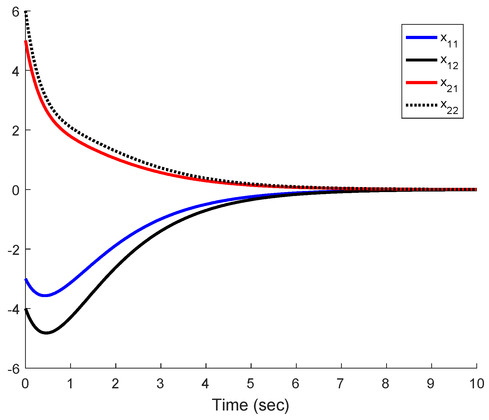
Consequently, we can conclude from Theorem 1 that the closed-loop system controlled by the decentralized static output gain $K_d$ is asymptotically stable. Thus, we have been able to easily analyze the stability of the decentralized case from the stability property of the centralized one. Figure 1 shows the trajectories of the closed-loop system when the gain $K_d$ is deployed with initial conditions given by $x_1{(t)}^T=\left[\begin{array}{cc}-3& -4\end{array}\right]$, $x_2{(t)}^T=\left[\begin{array}{cc}5& 6\end{array}\right]$. It can be observed in Figure 1 that all the states converge to zero as predicted by Theorem 1.

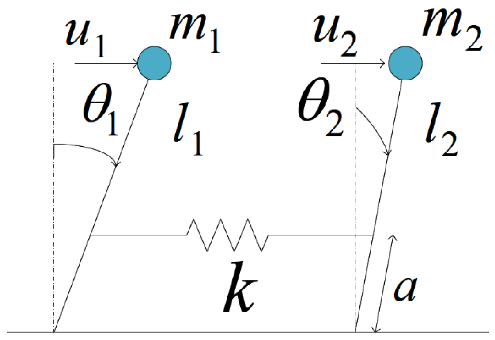
Example 2.

Consider the linear system with the same number of inputs and outputs composed of two identical pendulums THAT are coupled by a spring and subject to two distinct inputs, as displayed in Figure 2, [19].

The mathematical model of such interconnected system is given by:

$$\begin{array}{l}{\dot{x}}_1(t)=A_{11}{x}_1(t)+A_{12}{x}_2(t)+B_1{u}_1(t)\\ {\dot{x}}_2(t)=A_{21}{x}_1(t)+A_{22}{x}_2(t)+B_2{u}_2(t)\\ y_1(t)=C_1{x}_1(t)\\ y_2(t)=C_2{x}_2(t)\end{array}$$

with $x_1{(t)}^T=\left[\begin{array}{cc}{\theta }_1& {\dot{\theta }}_1\end{array}\right]$, $x_2{(t)}^T=\left[\begin{array}{cc}{\theta }_2& {\dot{\theta }}_2\end{array}\right]$ and matrices defined by:

$$A_{11}=A_{22}=\left[\begin{array}{cc}0& 1\\ \frac{g}{l}-\frac{k{a}^2}{m{l}^2}& -\mu \end{array}\right],\hspace{0.17em}{A}_{12}=A_{21}=\left[\begin{array}{cc}0& 0\\ \frac{k{a}^2}{m{l}^2}& 0\end{array}\right], B_1=B_2=\left[\begin{array}{c}0\\ \frac{1}{m{l}^2}\end{array}\right]$$

$$C_1=C_2=\left[\begin{array}{cc}1& 0\end{array}\right]$$

where g represents the gravity, $\mu$ accounts for the friction, $m=m_1=m_2$ are the masses of both pendulums, k is the spring constant and the meanings of the geometrical parameters are shown in Figure 2. This linear model corresponds to the linearization of the pendulum nonlinear equations around the up-right position equilibrium point. The following values were used in simulation, [19]:

$$\frac{g}{l}=1,\hspace{0.17em}\frac{1}{m{l}^2}=1,\hspace{0.17em}\mu =1,\hspace{0.17em}\frac{k}{m}=2,\hspace{0.17em}\frac{a}{l}=0.5$$

This system can be cast into the form of Equations (1) and (2) as:

$$A_c=\left[\begin{array}{cccc}0& 1& 0& 0\\ 0.5& -1& 0.5& 0\\ 0& 0& 0& 1\\ 0.5& 0& 0.5& -1\end{array}\right], B_c=\left[\begin{array}{cc}0& 0\\ 1& 0\\ 0& 0\\ 0& 1\end{array}\right], C_c=\left[\begin{array}{cccc}1& 0& 0& 0\\ 0& 0& 1& 0\end{array}\right], D_c=0$$

A static output feedback controller can be designed for this system to achieve its asymptotic stability. In this way, the feedback gain

$$K_c=\left[\begin{array}{cc}2.92& 0.65\\ 0.64& 2.80\end{array}\right]$$

places the closed-loop poles at $\left\{-0.5\pm 1.5i,-0.5\pm 1.4i\right\}$ with negative real parts. Now, we implement a decentralized controller with feedback gain given by:

$$K_d=\left[\begin{array}{cc}2.92& 0\\ 0& 2.80\end{array}\right]$$

Theorem 2 is now used to analyze the stability of the closed-loop system when this controller is employed. This case is of practical importance and corresponds to the situation when the local controller has only available for control purposes the information regarding the local output, and not the output of the complete system. Thus, the centralized and decentralized systems are the same and only the static feedback gain changes. Theorem 2 conditions are applied with ${\tilde{\sigma }}_A={\tilde{\sigma }}_B={\tilde{\sigma }}_C={\tilde{\sigma }}_D=0$, ${\tilde{\sigma }}_K={\Vert K_c-K_d\Vert }_2=0.65$ while the stability condition for this special case (see Appendix B) reads:

$$0.65=0.65\times 1\times 1={\Vert K_c-K_d\Vert }_2{\Vert B_c\Vert }_2{\Vert C_c\Vert }_2<1$$

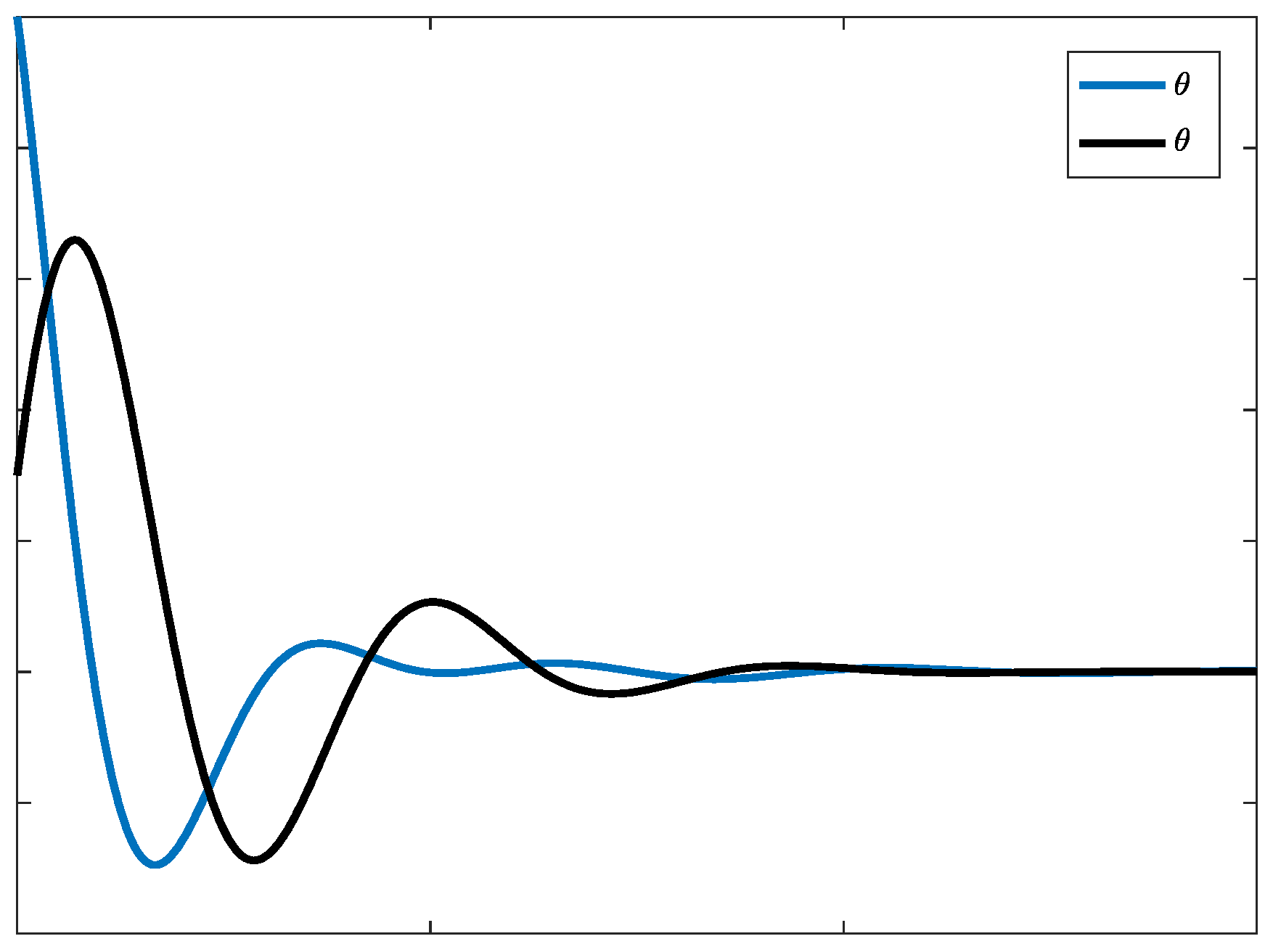
Accordingly, the closed-loop system attained with the decentralized controller is asymptotically stable and all the outputs will converge to zero asymptotically. Figure 3 displays the evolution of both angles from initial conditions $x_1{(t)}^T=\left[\begin{array}{cc}0.5& -0.5\end{array}\right]$, $x_2{(t)}^T=\left[\begin{array}{cc}0.15& 0.5\end{array}\right]$, where it can be observed that both pendulums are stabilized in the up-right position with the decentralized controller.

Example 3.

Consider the linear interconnected system given by:

$$\begin{array}{l}{\dot{x}}_c(t)=A_c{x}_c(t)+B_c{u}_c(t)\\ y_c(t)=C_c{x}_c(t)+D_c{u}_c(t)\end{array}$$

with matrices defined by:

$$A_c=\left[\begin{array}{ccc}-1& 0.4& 0.3\\ 0.2& -2& 0.1\\ -0.1& 0.2& -3\end{array}\right],B_c=\left[\begin{array}{ccc}1& 0.1& 0\\ 0& 2& 0\\ 0& 0& 2\end{array}\right],C_c=\left[\begin{array}{ccc}1& 0.1& 0\\ 0& 1& 0.1\\ 0& 0& 1\end{array}\right],D_c=0.1I_3$$

This system is controlled by the static output feedback gain given by:

$$K_c=\left[\begin{array}{ccc}0.19& 0.05& 0.04\\ 0.05& -0.01& 0.03\\ -0.02& 0.02& -0.46\end{array}\right]$$

which places the closed-loop poles at $\left\{-1.17,-2,-2.1\right\}$. The decentralized system is now given by:

$$A_d=A_c,B_d=\left[\begin{array}{ccc}1& 0& 0\\ 0& 2& 0\\ 0& 0& 2\end{array}\right],\hspace{0.17em}{C}_d=I_3,\hspace{0.17em}{D}_d=0$$

The decentralized system corresponds to the case when some transmission links have been suppressed from the original open-loop coupled dynamics, as considered in Remark 2. The following decentralized gain iz employed to stabilize the decentralized system in Equations (4)–(6) parameterized by the above matrices:

$$K_d=\left[\begin{array}{ccc}0.19& 0& 0\\ 0& -0.01& 0\\ 0& 0& -0.46\end{array}\right]$$

Theorem 2 is used to analyze the stability of the decentralized closed-loop system. To this end, we calculate:

$${\Vert A_c-A_d\Vert }_2={\tilde{\sigma }}_A=0$$

$$0.1={\Vert B_c-B_d\Vert }_2\le {\tilde{\sigma }}_B\epsilon =2.7\times 0.07=0.19$$

$$0.1={\Vert C_c-C_d\Vert }_2\le {\tilde{\sigma }}_C\epsilon =2.7\times 0.07=0.19$$

$$0.1={\Vert D_c-D_d\Vert }_2\le {\tilde{\sigma }}_D\epsilon =2.7\times 0.07=0.19$$

$$0.07={\Vert K_c-K_d\Vert }_2\le {\tilde{\sigma }}_K\epsilon =2.7\times 0.07=0.19$$

With these values, we can compute $\overline{\epsilon }=0.31,\hspace{0.17em}{\overline{\epsilon }}_1=0.24,\hspace{0.17em}{\overline{\epsilon }}_2=0.071$ so that $0.07=\epsilon <{\overline{\epsilon }}^{\ast }=min\left(1,\overline{\epsilon },{\overline{\epsilon }}_1,{\overline{\epsilon }}_2\right)=0.071$. Since ${\Vert K_c{D}_c\Vert }_2=0.05<1$, we are in conditions of applying Theorem 2 (i) and we can conclude that the decentralized closed-loop system is asymptotically stable. In this way, the presented results allow establishing the stability of the decentralized system by a simple method based on the stability and design of the centralized system. 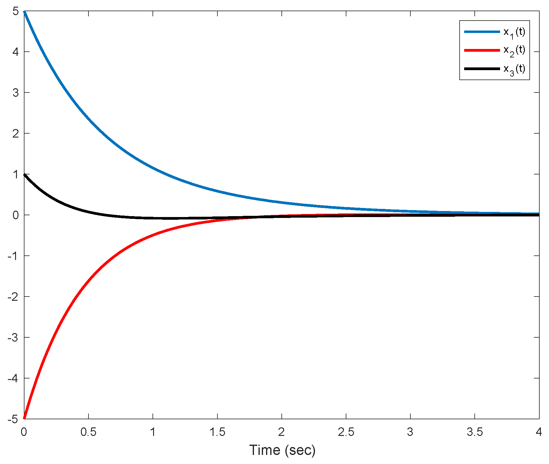Figure 4 shows the state variables evolution from the initial state $x{(t)}^T=\left[\begin{array}{ccc}5& -5& 1\end{array}\right]$. As shown in Figure 4, the state variables converge to zero asymptotically, as concluded from Theorem 2.

5. Concluding Remarks

This paper is devoted to formulating sufficiency-type linear-output feedback decentralized closed-loop stabilization conditions if the continuous-time linear dynamic system can be stabilized under linear output-feedback centralized stabilization. The developed stability tests are conceptually simple to evaluate and they rely on the quantification in terms of worst-case norms of interconnection and open-loop system dynamics matrices and the corresponding control gains in the decentralized case compared to the centralized counterpart. The tolerances of the various parametrical matrix errors have been quantified by considering the first or second powers of a small parameter. Such a parameter is a design factor to characterize in the worst-case for the allowed tolerances to the perturbed parameterization norms. Simulated examples are discussed to illustrate the obtained results. The decentralized control design versus its decentralized control counterpart, under eventual output linear feedback, has been studied from the point of view of the amount of information that can be lost or omitted in terms of the total or partial knowledge of the coupled dynamics between subsystems necessary in the decentralized case to keep the closed-loop stability. A foreseen related future work relies on the application of the method to some applied control problems such as consensus protocols under decentralized control and continuous-discrete hybrid controller designs.

References

1. Ibeas, A.; de la Sen, M. Robustly stable adaptive control of a tandem of master-slave robotic manipulators with force reflection by using a multiestimation scheme. IEEE Trans. Cybern. Part B Cybern. 2006, 36, 1162–1164. [Google Scholar] [CrossRef]
2. Barambones, O.; Garrido, A.J.; Garrido, I. Robust speed estimation and control of an induction motor drive based on artificial neural networks. Int. J. Adapt. Control Signal Process. 2008, 22, 440–444. [Google Scholar] [CrossRef]
3. Bakule, L.; de la Sen, M. Decentralized stabilization of networked complex composite systems with nonlinear perturbations. In Proceedings of the 2009 International Conference on Control and Automation, Christchurch, New Zealand, 9–11 December 2009; Volume 1–3, pp. 2272–2277. [Google Scholar]
4. Singh, M.G. Decentralised Control; North-Holland Systems and Control Series; North Holland Publishing Company: New York, NY, USA, 1981; Volume 1. [Google Scholar]
5. Berman, A.; Plemmons, R.J. Nonnegative Matrices in the Mathematical Sciences; Academic Press: New York, NY, USA, 1979. [Google Scholar]
6. Kailath, T. Linear Systems; Prentice-Hall Inc.: Englewood Cliffs, NJ, USA, 1980. [Google Scholar]
7. Ortega, J.M. Numerical Analysis; Academic Press: New York, NY, USA, 1972. [Google Scholar]
8. Shi, H.; Li, P.; Wang, L.; Su, C.; Yu, J.; Cao, J. Delay-range-dependent robust constrained model predictive control for industrial processes with uncertainties and unknown disturbances. Complexity 2019, 2019, 2152014. [Google Scholar] [CrossRef]
9. Rosas-Jaimes, O.A.; Munoz-Hernandez, G.A.; Mino-Aguilar, G.; Castaneda-Camacho, J.; Gracios-Marin, C.A. Evaluating fractional PID control in a nonlinear MIMO model of a hydroelectric power station. Complexity 2019, 2019, 9367291. [Google Scholar] [CrossRef]
10. Xu, L.; Lou, S.; Xu, P.; Zhang, G. Feedback control and parameter invasion for a discrete competitive Lotka-Volterra system. Discret. Dyn. Nat. Soc. 2018, 2018, 7473208. [Google Scholar] [CrossRef]
11. Rana, S.M.S. Chaotic dynamics and control of discrete ratio-dependent predator-prey system. Discret. Dyn. Nat. Soc. 2017, 2017, 4537450. [Google Scholar] [CrossRef]
12. Hassan, A.; Dvorkin, Y.; Deka, D.; Chertkov, M. Chance-constrained ADMM approach for decentralized control of distributed energy resources. In Proceedings of the 2018 Power Systems Computation Conference (PSCC), Dublin, Ireland, 11–15 June 2018; pp. 1–7. [Google Scholar]
13. Shao, S.; Yang, H.; Jiang, B.; Cheng, S. Decentralized fault tolerant control for a class of interconnected nonlinear systems. IEEE Trans. Cybern. 2018, 48, 178–186. [Google Scholar] [CrossRef] [PubMed]
14. Nayyar, N.; Kalathil, D.; Jain, R. Optimal decentralized control with asymmetric one-step delayed information sharing. IEEE Trans. Control Netw. Syst. 2018, 5, 653–654. [Google Scholar] [CrossRef]
15. Wei, C.; Luo, J.; Yin, Z.; Wei, X.; Yuan, J. Robust estimation-free decentralized prescribed performance control of nonaffine nonlinear large-scale systems. Int. J. Robust Nonlinear Control 2018, 28, 174–196. [Google Scholar] [CrossRef]
16. Wang, Y.; Lopez, J.A.; Sznaier, M. Convex optimization approaches to information structured decentralized control. IEEE Trans. Autom. Control 2018, 63, 3393–3403. [Google Scholar] [CrossRef]
17. Zhang, H.G.; Yu, H.; Hao, F. Decentralized integral-based event-triggered stabilization for linear plant with actuator saturation and output feedback. Appl. Sci. 2017, 7, 11. [Google Scholar] [CrossRef]
18. Lotfy, M.E.; Senjyu, T.; Farahat, M.A.F.; Abdel-Gawad, A.F.; Lei, L.; Datta, M. Hybrid genetic algorithm fuzzy-based control schemes for small power system with high penetration wind farms. Appl. Sci. 2018, 8, 373. [Google Scholar] [CrossRef]
19. Fu, Q.; Gu, P.; Wu, J.-R. Decentralized Iterative Learning Control for Large-scale Interconnected Linear Systems with Fixed Initial Shifts. Int. J. Control. Syst. 2017, 15, 1991–1994. [Google Scholar] [CrossRef]
20. He, W.; Dong, Y. Adaptive fuzzy neural network control for a constrained robot using impedance learning. IEEE Trans. Neural Netw. Learn. Syst. 2018, 29, 1174–1186. [Google Scholar] [CrossRef] [PubMed]
21. He, W.; Dong, Y. Design and adaptive control for an upper limb robotic exoskeleton in presence of input saturation. IEEE Trans. Neural Netw. Learn. Syst. 2019, 30, 97–108. [Google Scholar] [CrossRef] [PubMed]
Figure 1. States evolution when the decentralized controller K d is employed.
Applsci 09 01739 g001
Figure 2. Two inverted pendulums coupled by a spring.
Applsci 09 01739 g002
Figure 3. Evolution of the angles of both pendulums.
Applsci 09 01739 g003
Figure 4. Evolution of the state space variables when the decentralized controller K d is used.
Applsci 09 01739 g004