Article

Automatic Spatial Audio Scene Classification in Binaural Recordings of Music †

by
Sławomir K. Zieliński
1 and
Hyunkook Lee
2,*
1
Faculty of Computer Science, Białystok University of Technology, 15-351 Białystok, Poland
2
Applied Psychoacoustics Laboratory (APL), University of Huddersfield, Huddersfield HD1 3DH, UK
*
Author to whom correspondence should be addressed.
Binaural audio corpus, database with extracted features, and machine-learning code is available at: 10.5281/zenodo.2639058.
Appl. Sci. 2019, 9(9), 1724; https://doi.org/10.3390/app9091724
Submission received: 4 April 2019 / Revised: 18 April 2019 / Accepted: 19 April 2019 / Published: 26 April 2019
(This article belongs to the Special Issue Psychoacoustic Engineering and Applications)

Abstract

:
The aim of the study was to develop a method for automatic classification of the three spatial audio scenes, differing in horizontal distribution of foreground and background audio content around a listener in binaurally rendered recordings of music. For the purpose of the study, audio recordings were synthesized using thirteen sets of binaural-room-impulse-responses (BRIRs), representing room acoustics of both semi-anechoic and reverberant venues. Head movements were not considered in the study. The proposed method was assumption-free with regards to the number and characteristics of the audio sources. A least absolute shrinkage and selection operator was employed as a classifier. According to the results, it is possible to automatically identify the spatial scenes using a combination of binaural and spectro-temporal features. The method exhibits a satisfactory classification accuracy when it is trained and then tested on different stimuli but synthesized using the same BRIRs (accuracy ranging from 74% to 98%), even in highly reverberant conditions. However, the generalizability of the method needs to be further improved. This study demonstrates that in addition to the binaural cues, the Mel-frequency cepstral coefficients constitute an important carrier of spatial information, imperative for the classification of spatial audio scenes.

1. Introduction

1.1. Background

Binaural audio technology is rapidly gaining popularity. For example, it is now widely used for the rendering of 360° virtual reality content in one of the most popular video-sharing Internet services [1]. In their pilot experiment, Research and Development Department of the British Broadcasting Corporation (BBC R&D) has recently produced some of the most prominent classical music concerts in a binaural format [2]. Furthermore, binaural technology is now supported in one of the commonly used web browsers, allowing for real-time rendering of spatial audio scenes [3]. The interested reader is referred to [4] for an overview of the techniques used to record, reproduce, or synthesize binaural signals.
Due to the increasing number of applications adopting binaural technology, it is expected that large repositories of binaural recordings will soon be created. This may give rise to challenges concerning semantic search and retrieval of spatial audio content. For example, a hypothetical user of future multimedia systems may search the Internet resources for binaural audio recordings not only according to genre (pop music, jazz, sound effects, etc.) but also with regards to their spatial properties (e.g., audio clips with prominent audio content arriving from above or from behind of the head).
According to Rumsey’s spatial audio scene-based paradigm [5], complex spatial audio scenes could be described using perceptual attributes describing (1) individual audio sources, (2) ensembles of sources, and (3) acoustic environments. However, most of the models, mimicking spatial hearing in humans, are limited to the localization of individual audio sources [6,7,8,9,10], ignoring higher-level attributes describing complex spatial audio scenes.
Early machine-listening algorithms, inspired by spatial hearing in humans, could be characterized as single-source localization models since they were capable of localization of only one audio source at a time [11,12]. More recently, multiple-source localization models have been developed [6,7,8,9], which constitutes an important step towards quantification of higher-level attributes (e.g., ensemble width), ultimately leading to a holistic characterization of complex spatial audio scenes. While their reported accuracy is deemed to be good, their applicability is limited, as they often require a priori knowledge about the number of sources of interest and their signal characteristics. Another drawback of the multiple-source binaural localization models is that they were developed and tested predominately using speech signals [6,7,8,9]. Hence, their applicability to music recordings is unknown.
With the exception of the early models [11,12], it is now a common practice to employ artificial intelligence-based algorithms in machine-listening systems. They typically include such algorithms as Gaussian mixture models [6] and neural networks [10]. In line with the recent trends in machine learning, deep neural networks and convolutional networks have also been applied to binaural models [7,8,13].
It is widely accepted that there are three types of binaural cues responsible for spatial hearing in humans, namely: interaural level difference (ILD), interaural time difference (ITD), and interaural coherence (IC) [14]. While ILD and ITD are predominantly responsible for localization of audio sources in the horizontal plane, IC affects the apparent source width [15]. In addition to binaural cues, spectral cues help humans to localize sources in the sagittal plane [16] and provide help in front–back disambiguation [14].
There are two factors potentially hindering the performance of binaural models, namely a front–back confusion effect [14] and acoustic reverberations (room reflections) combined with background noise. While artificially simulated head movements could reduce the localization error [6], such systems require access to a motorized dummy-head microphone [17] or necessitate the incorporation of a spatial audio renderer, essential for a dynamic synthesis of binaural stimuli with simulated head rotation [6]. The adverse influence of reverberations on performance of binaural models could be partially reduced by processing direct sounds and room reflections separately. However, a decomposition of audio recordings into their prime and ambient components still constitutes a challenging task [18]. The other solutions involve a so-called multi-conditional training [6] or incorporation of a precedence effect model [19].
In summary, over the past two decades, substantial improvements have been made with regards to binaural modelling of human hearing, in particular in relation to localization of multiple speakers in binaural speech signals [6,7,8,9]. However, to the best of the authors’ knowledge, no formal studies towards the automatic characterization of complex audio scenes in binaural recordings of music have been reported yet, with the exception of the paper summarizing the pilot experiment undertaken by the present authors [20].
The real-world binaural recordings, acquired predominantly from the publicly available Internet repositories, were exploited in the aforementioned pilot experiment [20]. The number of excerpts used in the previous study was relatively small (600), making it difficult to train the model and then to reliably validate it. Moreover, these recordings were annotated manually by the first author, potentially introducing some level of researcher bias. Furthermore, an analysis of the importance of the extracted features revealed the surprising prevalence of spectro-temporal metrics over the binaural cues, which might have been caused by genre imbalance (spectral cues are known to be instrumental in the area of music genre classification [21]). For example, one of the scenes was overrepresented by environmental recordings (soundscapes), whereas another scene was dominated by pop music excerpts. Therefore, it could be hypothesized that the classifier used in the pilot experiment might have worked, to some extent, as a genre recognizer rather than as a spatial scene classifier. In order to circumvent the drawbacks of the pilot test, it was necessary to repeat the experiments using a large number of contrived excerpts (as opposed to a small set of real-world recordings), with an equal number of genre types for each spatial scene and with a controlled horizontal distribution of audio sources around a listener. The above considerations underlay the work described in this paper.

1.2. Aims of the Study

From the above background, the current study proposes a novel method that automatically categorizes binaural recordings of music according to the horizontal distribution of foreground audio content (ensemble of musicians) and background audio components (room reflections) around a listener. The study also compares the influence of several groups of features, extracted from binaural recordings, on the classification accuracy of the proposed method. The following groups of metrics were incorporated in this work: binaural, spectro-temporal, Mel-frequency cepstral coefficients (MFCCs), and descriptors based on the root mean square (RMS) values of the signals.
The proposed method could be incorporated in the algorithms used for semantic search and retrieval of audio content. It might also be used as a spatial scene-detector in audio quality expert systems (the performance of spatial quality expert systems could be improved by providing them with information on spatial audio scene characteristics [22]). Moreover, it might be embedded to environment-aware signal processing algorithms, including binaural hearing aids, adapting their parameters depending on the surrounding audio scenes. It could also be used as a preselection tool for gathering audio material for subjective audio quality assessment tests.
This study builds on the work on the spatial audio scene characterization of five-channel surround sound recordings undertaken by Zieliński [23,24]. As mentioned above, it constitutes an extension of the preliminary work concerning the automatic categorization of binaural recordings, carried out by the present authors [20].
The paper is organized as follows: in Section 2, the topology of the algorithm, the audio corpus, and the classification algorithm are described; Section 3 presents the results; and Section 4 and Section 5 include discussion and conclusions, respectively.

2. Materials and Methods

In this section, an overview of the methods is provided, followed by a description of the binaural recordings, the feature extraction procedure, and the classification algorithm used in the study along with a rationale for its selection.

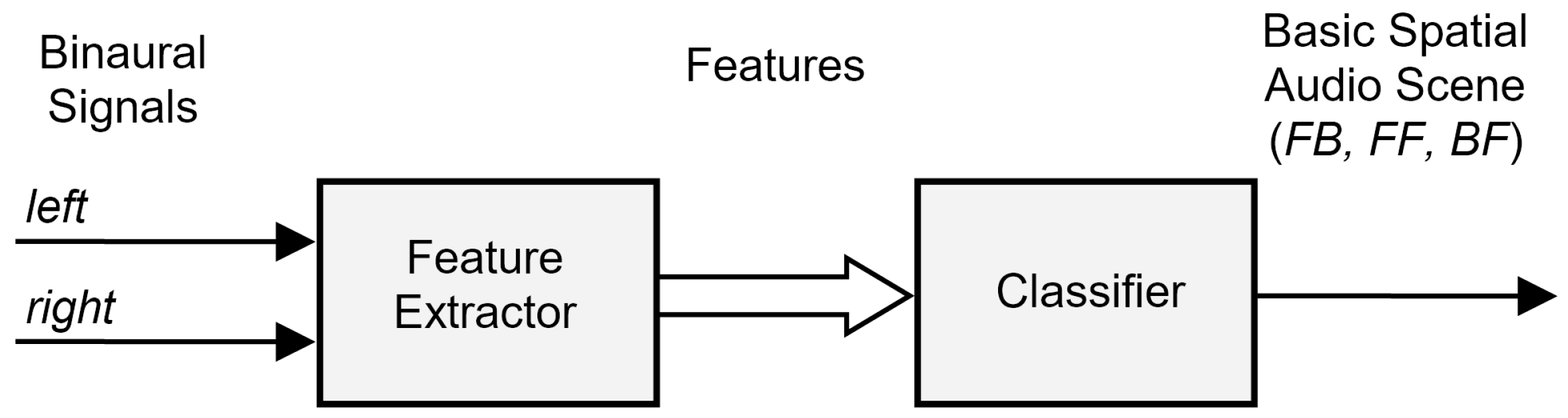
2.1. Method Overview

A traditional two-stage approach of manually designed feature extractor followed by a machine learning-based classifier was adopted in this study, as illustrated in Figure 1. Note that in the proposed topology no source separation algorithms, or any other sophisticated algorithms aiming to isolate and localize audio sources prior to their classification, were employed. Moreover, for the reasons explained earlier, it was decided to develop a method without simulating any head rotation effects, which further simplified the development. It was assumed by these authors that the proposed two-stage algorithm, simulating a stationary head scenario, would be adequate for the task of classifying spatial audio scenes.
Some of the recently developed methods for localization of audio sources in complex binaural recordings require a priori knowledge of a number of audio objects present in a spatial scene (e.g., [6]). No such requirement was imposed on this method. As it is shown in the remainder of the paper, the proposed method was successfully tested using binaural recordings with the number of audio sources ranging from 5 to 42.
The three basic spatial audio scenes were considered in this study, as overviewed in Table 1. They differed with respect to a horizontal distribution of foreground and background audio content. Foreground sound objects represented easily identifiable, important, and clearly perceived audio sources, whereas background objects normally represented reverberant, unimportant, unclear, ambient, “foggy”, and distant sound sources.
The first scene, referred to as foreground–background (FB), described a scenario where a listener perceived predominantly foreground audio content as arriving from the front and background audio content as originating from the back. It may represent a typical situation of a listener sitting in the audience and listening to the musicians located at the stage, e.g., during a classical music concert. By contrast, background–foreground (BF) scenes represented a “reversed” scenario, where background audio content arrived from the front and predominantly foreground audio content was perceived from the back (behind the head). This scene could be encountered in virtual reality applications, including computer games. The third scene, termed foreground–foreground (FF), described a situation where predominantly foreground audio content was perceived by a listener as arriving both from the front and from the back. It could be exemplified by a situation where a listener was surrounded by musicians. This scene could be often encountered in binaural pop music recordings.
The above categorization of spatial audio scenes was originally inspired by Rumsey’s spatial audio scene-based paradigm [5]. In a form limited to two categories (FB, FF), it was used by Beresford et al. [25] to label experimental recordings of classical music. A similar categorization of spatial scenes, although with a different nomenclature (“stage–audience recording scenario” versus “360° stage scenario”), was also adopted by Lee and Millns [26] in their experiment investigating 3D audio microphone techniques. Such categorization also proved to be useful in explaining empirical data acquired from the experiments with spatial sound [27]. As already mentioned in the Introduction, a performance of audio quality expert systems could be improved if information regarding a category of the basic spatial scene (FB or FF) was provided to their input [22].
In addition to the three categories of spatial audio scenes, already overviewed in Table 1, an extra (fourth) category was also used in our previous study [20]. It was signified as background–background (BB) and referred to a situation where a listener was surrounded solely by background audio objects. Such category was particularly relevant in the case of environmental recordings. Since the present study was limited to music recordings, such a scene could be regarded as of little relevance, and hence it was omitted as obsolete.
The methodological approach taken in this work was different compared to the one typically followed in the area of computational auditory scene analysis (CASA). The purpose of CASA is to decompose complex acoustical scenes into their elementary constituents [28], with a blind source separation (BSS) serving as an example [29]. In this study it was decided to undertake a classification of the spatial scenes without decomposition into their elementary components, hence omitting the CASA module. The proposed method was also different from the algorithms used in a rapidly growing area of acoustic scene classification (ASC) [30]. The purpose of ASC is to identify an environment in which the sound sources were recorded, whereas the objective of the proposed method is to classify spatial audio scenes with regards to a distribution pattern of a foreground and background audio content.

2.2. Corpus of Binaural Audio Recordings

This section provides a description of how the audio recordings were generated. Initially, it explains how the raw audio material was selected and preprocessed. Then, it describes the incorporated binaural-room-impulse-responses (BRIRs) as well as the spatial synthesis techniques employed in the study.

2.2.1. Raw Audio Material

The procedure used to generate the audio corpus was as follows. First, a group of 152 multitrack audio recordings was gathered, out of which 112 were selected for training, whereas the remaining 40 items were allocated for testing. They included anechoic and semi-anechoic recordings of classical music orchestra [31] and opera [32]. They also contained typical multitrack studio recordings representing such music genres as pop, orchestral, jazz, country, electronica, dance, rock, and heavy metal. All the recordings were acquired from the publicly available repositories [33,34,35]. For most of the selected multitrack recordings, each track represented a single musician or an individual musical instrument. If a given instrument was recorded stereophonically on two tracks, the signals from these tracks were down-mixed to a single monophonic track. It is a common practice taken by sound engineers to record drum-kits using several separate tracks. In this experiment, such tracks were mixed with equal gains to monophonic signals so that the whole drum-kit was stored on a single monophonic track. After such preprocessing, it was assumed by the authors that every monophonic track in the selected multitrack recordings represented an individual foreground audio object, be it a singer or a musical instrument. Finally, all the tracks were RMS-level normalized and stored as separate uncompressed audio files with 24-bit resolution at a 48 kHz sample rate.

2.2.2. Database of Binaural Room Impulse Responses

Table 2 gives an overview of the thirteen databases of BRIRs used to synthesize binaural recordings. The exploited BRIRs represented a broad range of acoustical and technical conditions (venues and dummy heads), which was essential in order to reliably validate the inter-BRIR generalizability of the proposed method. It can be seen in the table that the reverberation time (RT60) of the BRIRs ranged from 0.17 to 2.1 s. The three types of dummy heads were used to capture the BRIRs, namely B&K HATS Type 4100, Neumann KU100, and KEMAR 45BA. It was hypothesized by these authors that the head-and-torso simulators might have “imprinted” some spatial or spectral characteristics onto the BRIRs, and, therefore, it was decided to include in the experiments the BRIRs captured using at least three types of dummy heads.
The BRIRs used in the study also differed in terms of their spatial resolution. In the case of the BRIR set No. 1 (sbs), 15 measurement positions were available [36]. However, in order to maintain front–back symmetry, only 8 BRIRs, out of 15, were incorporated in the study. They represented an octagonal configuration of loudspeakers, with the speakers positioned horizontally at the angles equal to 0, ±45°, ±90°, ±135°, and 180°, respectively. A similar, octagonal configuration was also adopted in the case of the BRIR set No. 2 (mair) [26].
For the BRIR sets Nos. 3 and 4 (thkcr1 and thkcr7) [37], binaural impulse responses from only two physical loudspeakers were available, positioned at the angles of ±30°, respectively, which was adequate to synthesize the FB scene. In order to extract BRIRs for “missing” rear loudspeakers, indispensable to synthesize the remaining two scenes (BF and FF), binaural impulse responses obtained for the front physical loudspeakers were also exploited, however, with the data obtained using the dummy head rotated to 180°, and with the impulse responses between the left and right loudspeakers being swapped. In this paper, we refer to this technique as front–back “mirroring.” This approach could be legitimately used assuming that the dummy head was placed at the acoustical center of a room and also assuming room symmetry. Although these assumptions were moderately violated, it could be argued that while such procedure might have slightly affected the way room reflections were perceived, it did not influence the perception of the foreground audio content (due to front–back symmetry of the loudspeakers with respect to the dummy head), and hence did not affect the validity of this study. This supposition was confirmed by the informal listening tests undertaken by the authors.
In the case of the BRIR set No. 5 (thksbs), the three physical loudspeakers located at the front of a dummy head were used to capture the binaural responses [37]. These loudspeakers were positioned at the azimuth angles equal to 0° and ±28°, respectively. The next set of BRIRs (No. 6, thklbs) was obtained using only two physical loudspeakers, placed at the angles of −18 and 0°. They represented front–left and front–center loudspeakers, respectively. In line with the recommendation of the authors of that database [37], the binaural room response for the virtual front–right loudspeaker (+30°) was obtained by swapping front and left signals of the front–left loudspeaker (left–right “mirroring” technique). For both BRIR sets described above (Nos. 5 and 6), the binaural room responses for the virtual rear loudspeakers were obtained using the front–back mirroring technique.
The BRIR set No. 7 (calypso) contained the measurements acquired using a standard five-channel loudspeaker layout [38], with the speakers located at 0°, ±30°, and ±110°, respectively. Despite the lack of front–back symmetry in the loudspeaker layout, all the BRIRs from the above set were incorporated in the study. Informal auditioning of the synthesized stimuli, using the above BRIRs, revealed that the excerpts representing the BF scene had distinctively different timbral characteristics (being perceived as “duller”) and appeared to be elevated, compared to those exhibiting the FB scene. The elevation effect could be explained by the fact of using binaural responses from the widely spaced loudspeakers (±110°), as demonstrated by Lee [39].
The BRIR set No. 8 (tvtui) also contained the binaural impulse responses acquired using a standard five-channel loudspeaker layout, with the speakers located at 0°, ±30°, and ±120°, respectively [40]. In order to avoid the above-mentioned timbral coloration and the elevation effect, only the BRIRs from the three frontal loudspeakers were retained in the study (angles of 0° and ±30°). The binaural impulse responses of the virtual rear loudspeakers were generated using the front–back mirroring technique.
In the case of the BRIR set No. 9 (tvtui2) [41], the measurements were undertaken in the same venue (TV studio) as in the case of the previous set. However, in contrast to the previous BRIR set, the distance between the dummy head and the loudspeakers was reduced from 3.5 to 2 m. Moreover, a different loudspeaker type was utilized. In the case of the BRIR set No. 9 the measurements from 10 loudspeakers were provided, with 5 loudspeakers placed at the front (at the directions of 0°, ±15°, ±30°, respectively) and the remaining 5 loudspeakers positioned symmetrically at the back. All the measurements were incorporated into the study. In the case of the BRIR sets Nos. 10 and 11 (labtui and rehabtui), the same measurement layout was used as in the previous set (10 loudspeakers). The BRIRs contained in these two sets were captured in the listening room and the rehabilitation laboratory, respectively [41].
The last two sets of BRIRs (Nos. 12 and 13), signified as tuburo250 and tuboro310, contained the measurements from a 64-channel loudspeaker array of rectangular shape, intended to use for wave-field synthesis. For both sets the measurements were undertaken in the same laboratory, but with different levels of acoustical dumping, resulting in two different reverberation times equal to 250 and 310 ms, respectively [42].

2.2.3. Synthesis of Binaural Recordings

In order to synthesize the binaural recordings, monaural signals, representing individual foreground objects in raw audio material, were convolved with binaural impulse responses estimated for selected angles of incidence. Since the spatial resolution of the incorporated sets of BRIRs was low, with the exception of the last two sets of BRIRs, the binaural room responses for selected angles of incidence were calculated using the two techniques. For the BRIR sets Nos. 1–11, a standard vector-base amplitude-panning algorithm [43] was used to “interpolate” impulse responses. To this end, a MATLAB procedure written by Politis was utilized [44]. For the remaining two sets of BRIRs (Nos 12 and 13), the wave-field synthesis algorithm was exploited, using the MATLAB sound field synthesis toolbox developed by Wierstorf and Spors [45]. In the latter case, the virtual audio objects were synthesized as point sources at an intended distance of 3 m from a listener.
According to the description of the FB scene, presented earlier in Table 1, foreground audio objects could be, in theory, placed anywhere on the frontal half-plane. However, for simplicity, it was decided to limit the domain of possible placements (positions) to the frontal semicircle. Moreover, the panning angle was reduced from ±90° to ±30°, with 0° being the direction indicated by a listener’s nose. Some of the BRIRs employed in this study did not allow the use of panning angles beyond the limits of ±30°. Therefore, such restriction seemed to be a reasonable compromise between the need to span the azimuth range to a full semicircle and the necessity to validate the inter-BRIR generalizability of the method. The latter requirement implied that a relatively large number of BRIRs had to be included in the study. Note that after introducing the above simplifications, the resultant scenes still met the constraints of the basic spatial audio scene definitions, presented in Table 1.
Interestingly, informal listening tests undertaken by these authors indicated that despite the restriction of the azimuth range to ±30°, the perceived panning angle of the synthesized complex binaural recordings was wider than the intended one, for some stimuli appearing to span almost all frontal semicircle (±90°). The investigation of the discrepancy between the intended and the perceived ensemble width in binaurally synthesized stimuli is beyond the scope of this study.
As mentioned above, for the FB scenes, the intended directions of sound incidence for foreground objects were limited to ±30° (inclusive). This condition was illustrated in Figure 2a for a recording consisting of 20 foreground audio objects. For the BRIR sets Nos. 5 and 6, the panning angle had to be further reduced to ±28 and ±18°, respectively, due to the reduced spacing of the physical loudspeakers. No spacing restrictions, understood as a minimum angular difference between adjacent objects, were imposed on the randomly generated distribution patterns. For the BF scene, the panning angle was adjusted to the range between 150° and 210° in order to symmetrically “mirror” the FB scene. Examples of the intended azimuth angle distributions for the BF and FF scenes were illustrated on panels b and c in Figure 2, respectively. For the FF scene, audio objects were equally split between the front and back sectors in order to balance the number of objects in both sectors. For recordings containing an odd number of tracks, one of the objects was randomly allocated either to the front or to the back sector. In the case of the algorithm developed for the purpose of this study, intended azimuth angles were selected randomly and separately for each raw recording, so that there were no repeating spatial patterns across the synthesized excerpts.
The duration of the synthesized excerpts was limited to seven seconds. A sine-squared fade-in and fade-out, of 10 ms in duration, was applied to all the synthesized recordings.
The number of individual foreground audio objects in the group of recordings intended for training ranged from 5 to 62, with a median of 9. In the case of the recordings selected for testing, the number of foreground objects varied from 5 to 42, with a median number being equal to 10.
In total, 4368 excerpts were synthesized for training purposes (112 raw recordings × 3 scenes × 13 sets of BRIRs), whereas 1560 excerpts were synthesized to be used in testing procedures (40 raw recordings × 3 scenes × 13 sets of BRIRs). To allow other researchers to replicate the experiments described in this paper, the annotated corpus of all the binaural audio excerpts was made publicly available (10.5281/zenodo.2639058).

2.3. Feature Extraction

In total, 1376 features were extracted from all of the binaural audio excerpts. All the features could be divided into two categories: spatial and spectro-temporal. An overview of the extracted metrics is presented in Table 3. Regardless of the category, the features were extracted directly from the left and right channel signals—denoted as x and y, respectively—as well as from the mid (m) and side (s) signals, where m = x + y and s = xy. Prior to calculating the features, the signals were divided into 20 ms time frames with a 10 ms overlap. A Hamming window was applied to each frame. Details of the extracted features are described in the following subsections.

2.3.1. Root Mean Square (RMS) Features

The first group of spatial features was derived from the RMS values of the signals. They were included in the study in order to check whether such simple metrics would be useful to differentiate between the spatial scenes.
For each timeframe, a ratio between the RMS values of the x and y signals was computed (expressed in dB). It was referred to as x-to-y RMS ratio. This descriptor constituted a crude approximation of the interaural level differences (ILDs). Similarly, for every timeframe, a ratio between m and s signals was also calculated. This metric was termed m-to-s RMS ratio. It was assumed by the authors that this ratio could also be considered to be a simple descriptor of spatial characteristics.
All the metrics were calculated on a frame-by-frame basis. Then, they were summarized using the absolute mean values, yielding two metrics (one for the x-to-y RMS ratio another one for the m-to-s RMS ratio). In addition, they were also summarized by calculating the standard deviations, producing the two extra metrics. In order to account for temporal fluctuations of the RMS ratio across the timeframes, the standard delta metrics [46] were also computed in a similar way, as explained above, adding four more descriptors. The number of frames over which the delta features were computed (so-called delta width) was equal to two. Hence, the above procedure produced eight RMS-based features in total.

2.3.2. Binaural Cues

In order to extract the binaural cues, the signals were first band-pass filtered using a 42-channel gammatone filter bank with the lowest and the highest center frequencies of the filters being equal to 50 Hz and 16 kHz, respectively. Then, the inner hair-cell envelope of the bandpass filtered signals was extracted using the method consisting in half-wave rectification of the signals followed by their low-pass filtering with a cut-off frequency being equal to 1000 Hz, as proposed by Dau [47]. Next, the rate-maps were calculated. The rate-maps constituted a representation of auditory nerve firing rates [48]. The obtained rate-maps formed a basis for calculating the binaural cues (ILD, ITD, and IC). In addition to the above features, the standard delta metrics were also computed.
The binaural cues were estimated using the publicly available software package developed as an auditory front-end of the TWO!EARS system [17]. The same software was also utilized to calculate the spectral features described in the next subsection.
In summary, the following binaural cues were derived:
(1)
means and standard deviations of the ILD values calculated separately for each of the 42 gammotone filters (2 × 42 features),
(2)
means and standard deviations of the ITD values calculated separately for each of the 42 gammotone filters (2 × 42 features),
(3)
means and standard deviations of the IC values calculated separately for each of the 42 gammotone filters (2 × 42 features),
The above procedure yielded 252 metrics (3 × 2 × 42 features). In addition, in a similar way, the delta values were calculated, which doubled the number of metrics. Hence, in total 504 binaural features were produced.

2.3.3. Spectral Features

The reason for including the spectral features in this study was an observation made, among others, by such researchers as George et al. [49] and Conetta at al. [50]. They found that in order to build reliable models accounting for spatial quality of sound, it is not sufficient to extract only spatial metrics of the signals, but it is also necessary to derive the timbral descriptors. The timbral characteristics of sound are often correlated with the spectral features [51]. Hence, it was assumed that in order to build a classifier of the spatial audio scenes, the spatial metrics should be supplemented by the spectral features.
The following 14 spectral features were included in the calculations: centroid, spread, brightness, high-frequency content, crest, decrease, entropy, flatness, irregularity, kurtosis, skewness, roll-off, flux, and variation. They all constituted the standard metrics commonly used in ASC algorithms and music information retrieval applications. Their mathematical definitions can be found elsewhere [51,52,53,54]. Although they are commonly referred to as “spectral features”, some of them also account for temporal characteristics of sound, e.g., flux. Therefore, these features, along with the metrics described below, were categorized in this paper using a joint term of “spectro-temporal” features (see Table 3).
In summary, the following descriptors were estimated:
(1)
means and standard deviations of 14 spectral features calculated for x signal (2 × 14 features),
(2)
means and standard deviations of 14 spectral features calculated for y signal (2 × 14 features),
(3)
means and standard deviations of 14 spectral features calculated for m signal (2 × 14 features),
(4)
means and standard deviations of 14 spectral features calculated for s signal (2 × 14 features).
Hence, in total 112 metrics were calculated. This number was doubled by including delta features. Therefore, the overall number of the spectral features amounted to 224.

2.3.4. Mel-Frequency Cepstral Coefficient (MFCC) Features

Mel-frequency cepstral coefficients are commonly used as spectral descriptors in the area of music genre recognition [21] as well as in the ASC algorithms [30]. Since they are very effective in “summarizing” a shape of the spectrum (spectral envelope), it could be tentatively hypothesized that they might also be useful in capturing some information regarding the influence of the head-related transfer functions on the spectral characteristics of binaural recordings (peaks and deeps across the frequency response). Hence, they could also represent some cues responsible for the front–back discrimination of the auditory objects. Consequently, it could be speculated that in addition to being effective spectral descriptors, the MFCCs might help to discriminate between FB and BF scenes.
In our study, 40 MFCCs were extracted from the m and s signals, respectively. Rank of the coefficients ranged from 1 to 40. The selection of such an unusually large number of coefficients was in line with the recent trend in speech and audio classification [55,56]. The zeroth coefficient, representing signal energy, was omitted. In summary, the following MFCC-based metrics were computed:
(1)
means and standard deviations of the 40 MFCCs derived from x signal (2 × 40 features),
(2)
means and standard deviations of the 40 MFCCs derived from y signal (2 × 40 features),
(3)
means and standard deviations of the 40 MFCCs derived from m signal (2 × 40 features),
(4)
means and standard deviations of the 40 MFCCs derived from s signal (2 × 40 features).
Therefore, the above procedure produced 320 features. Similar calculations were also performed for the delta-MFCCs, yielding additional 320 features (640 metrics in total).
The RMS-based metrics, binaural cues, spectral features, and MFCC-derived features were extracted separately from the training and testing binaural excerpts. They were stored in two datasets (spreadsheets), intended for training and testing, respectively. For research reproducibility purposes, both spreadsheets were included in the publicly available repository accompanying this paper.

2.4. Classification Algorithm
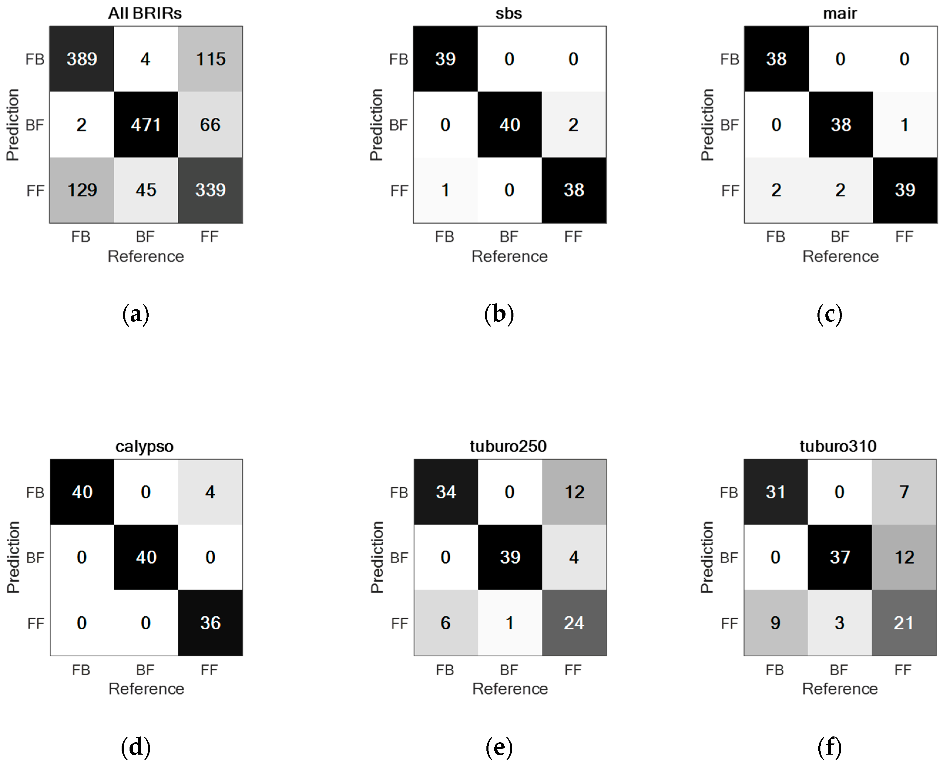
Prior to undertaking the classification procedure, all the features were standardized, yielding the column vectors with zero mean and unit variance. Due to its robustness against a multicollinearity effect [57], a least absolute shrinkage and selection operator (LASSO) was employed as a classification algorithm. Initial exploration of the data revealed that approximately 60% of the metrics were highly correlated (r > 0.8).
The second reason for using the LASSO algorithm was related to its inherent property of feature selection. Since this method exploited an L1 norm as a penalty criterion [58], it forced some of the regression coefficients to be exactly zero, hence “removing” the unnecessary metrics. Since the database used in the present study contained a large number of features (1376), the above property of the classification algorithm could, in theory, improve the generalizability of the model by reducing its number of degrees-of-freedom (parameters).
The hyper-parameters of the LASSO algorithm (alpha and lambda) were “tuned” using the standard 10-fold cross-validation procedure repeated 10 times. The selected values varied across the models (experiments), and, therefore, they will be provided in the next section.
The classification algorithm was implemented in R system using the caret package [59]. The code is openly available at Zenodo repository (10.5281/zenodo.2639058).

3. Results

This section contains the results of the two experiments. The aim of the first experiment was to check how the method performed when trained and tested on the excerpts synthesized using the same sets of BRIRs. Such an approach allowed to check the intra-BRIR generalizability of the method. Note that the testing and training datasets were mutually exclusive, with no common excerpts shared between the datasets. However, for the purposes of the first experiment, they were all synthesized using the same BRIRs. The aim of the second experiment was to test the method on the stimuli synthesized with the BRIRs “unseen” by the classification algorithm during its training. In this case, the inter-BRIR generalizability was evaluated.

3.1. Experiment 1

Table 4 summarizes the results obtained using a single model, trained and tested on the whole audio corpus (synthesized with all 13 BRIR sets). A classification accuracy reached the highest accuracy, equal to 81.2%, during the training of the model with all the features. However, the accuracy achieved upon testing was slightly lower and amounted to 76.9%. This outcome indicated that the model was slightly over-fit during the training. According to the results obtained upon testing, binaural cues played a dominant role in terms of the identification of the spatial scenes (accuracy of 73.1%), followed by MFCCs (69.0%), spectral features (52.2%), and RMS-based metrics (39.9%). The difference in accuracy values reached for the binaural metrics and the MFCCs, respectively, was statistically significant at p = 0.013 level, whereas the differences between the accuracy values obtained for MFCCs, spectral features, and RMS-based metrics were statistically significant at p < 10−11 level. Note that in this study the no-information rate was equal to 33.3%. Hence, the use of the RMS-based metrics in isolation from the other features yielded only a small improvement over the baseline value of 33.3%, with the accuracy being equal to 39.9%. This improvement was statistically significant at p = 2.8 × 10⁻⁸ level. The values of the hyper-parameters of the LASSO model (alpha and lambda), tuned during the cross-validation procedure, were equal to 0.55 and 3.094 × 10⁻³, respectively.
An interesting observation could be made by inspecting the data presented in Table 5 and Table 6. The tables present the accuracy results obtained during the training and testing procedures, respectively. In contrast to previously discussed Table 4, these tables illustrated the classification accuracy achieved using 13 BRIR-specific models. Each of the models was trained and tested with a different BRIR set. For example, the first row in Table 5 showed the performance of the model upon training using 336 audio excerpts synthesized with the BRIR set No. 1 (sbs). Similarly, the first row in Table 6 illustrated the accuracy obtained upon testing with the aforementioned model. Note that during the testing, another set of 120 stimuli was used. However, they were synthesized using the same BRIRs as upon training. It can be seen that the overall performance of the BRIR-specific models was markedly better compared to those obtained using a single model. According to the last column in Table 5, the classification accuracy of the individual models obtained during the training ranged from 71% to 97.8%. The accuracy of the BRIR-specific models reached upon testing varied from 74.2% to 98.3% (see the last column in Table 6). These outcomes implied that the classification model learned well the cues important for the discrimination between the spatial scenes within each BRIR set, however, it struggled to identify universal features required by a single, generic model.
A closer examination of the data presented in Table 5 and Table 6 revealed that for most of the models, the binaural cues played the most important role, in terms of the classification accuracy, followed by the MFCCs. The exceptions were the models obtained for the last two BRIR sets (Nos. 12 and 13) and the calypso BRIR set (No. 7). According to the statistical test of proportions, MFCCs were more prominent than the binaural cues (p = 8.9 × 10⁻³) for the model obtained for the BRIR set No. 12 (tuburo250). In the case of the models derived using the BRIR sets Nos. 7 and 13 (tuburo310 and calypso), no difference between the binaural cues and MFCCs could be statistically proven (p values equal to 1.0 and 0.56, respectively). Hence, it could be concluded that for the aforementioned two models, the MFCCs and the binaural cues were of similar importance.
For most of the BRIR-specific models, the RMS-based metrics and the spectral features appeared to be of little importance in terms of the classification accuracy. The exception was the model obtained for the BRIR set No. 7 (calypso), for which the accuracy attained for the spectral features and the RMS-based metrics was equal to 75.8% and 69.2%, respectively (see Table 6).
Figure 3 illustrates confusion matrices of the selected models. For example, the confusion matrix for the model trained using the audio excerpts synthesized with all the BRIR sets is presented on panel (a) of this figure. It showed that out of 520 recordings exhibiting the FB scene, 389 were classified correctly, 129 items were misclassified as representing the FF scene, while the remaining 2 excerpts were erroneously classified using the BF category. As far as the BF recordings were concerned, 471 ones were classified correctly, 45 recordings were incorrectly classified as FF, and the remaining 4 excerpts were misclassified as those exhibiting the FB scene. In the case of the FF recordings, 339 were classified correctly, 115 excerpts were misclassified as those representing the FB scene, and 66 as the recordings signifying the BF scene. Figure 3b shows that the model trained for the sbs BRIR set made only three mistakes. It correctly identified all the recordings exhibiting the BF scene. A good classification performance could also be observed in the case of the models obtained for the mair and calypso BRIR sets (Figure 3c,d), as most of the correctly identified recordings are placed on the diagonal of the confusion matrices. However, the confusion matrices obtained for the models trained using the tuburo250 and the tuburo310 BRIR sets showed an increased number of misclassified recordings. Nevertheless, all the confusion matrices illustrated in Figure 3 indicated that the models exhibited a high sensitivity with regards to the identification of the BF scene. Note that in the case of the models trained using the sbs and calypso BRIR sets, all the BF recordings were classified correctly. Likewise, the remaining models made a relatively small percentage of mistakes in this respect.

3.2. Experiment 2

The three tests were made to examine whether the method was capable to generalize when it was trained and then tested on the stimuli synthesized using different BRIR sets, but of similar reverberation time. The obtained results are presented in Table 7. For the first condition (short reverberation time), the model was trained using the stimuli synthesized with the following BRIR sets: sbs, thkcr1, calypso, labtui, and tuburo310. Then, it was tested employing the stimuli synthesized with the thkct7 and tuburo250 BRIR sets. According to the results, the model exhibited a moderate level of generalizability, yielding an accuracy level of 65.4%. For the remaining two conditions (medium and long reverberation times), the accuracy was low and equaled 51.7% and 40.0%, respectively. The above outcomes indicated that the method showed a moderate level of generalizability for the BRIR sets of short reverberation time, but it failed to generalize for the BRIRs representing medium or long reverberation times.
Other factors, extending beyond the acoustical conditions of the BRIR sets, may be of higher importance in terms of the generalizability of the method. For example, a surprisingly high classification accuracy, being equal to 82.5%, was obtained when the method was trained using the stimuli synthesized with the tuburo250 BRIR set and then tested on the recordings produced with the tuburo310 BRIR set. Although for these two BRIR sets the acoustical conditions were slightly different, in both cases the audio excerpts were generated using the wave-field synthesis method. This outcome indicated that the generalizability of the method may have strongly depended on the algorithm used to synthesize binaural audio recordings.
In order to test the inter-BRIR generalizability of the method in a more systematic way, a “leave-one-BRIR-out” validation technique was adopted. The procedure was applied iteratively, excluding one BRIR set from training in each iteration. The obtained results are presented in Table 8. For example, in the first iteration, the sbs BRIR set was left out, and the model was trained on the stimuli synthesized with all the remaining BRIR sets (12 sets in total), reaching a training accuracy of 80.8%. Then, the model was tested on the recordings synthesized using the previously excluded BRIR set (sbs in this case), yielding a testing accuracy of 44.2% (see the first row in Table 8). The procedure was repeated for the remaining BRIR sets. According to the third column in Table 8, the training accuracy for all the models was high, with an average value of 81.2%. However, the models exhibited an overfitting effect, as the testing accuracy was substantially less than the training accuracy (see the last column in the table). The best results were obtained for the tvtui2 BRIR set, with a testing accuracy reaching 79.2%, followed by the tuburo310 BRIR set yielding a test accuracy equal to 73.3%. By contrast, a testing accuracy obtained for the calypso and rehabtui BRIR sets was statistically not different from the no-information rate of 33.3% (p = 0.31). The average accuracy level obtained upon testing was equal to 56.8%.
In addition to testing the generalizability of the method, Table 8 could also be used to examine which BRIR sets were the most challenging in terms of the classification accuracy. At the outset of the study, it was expected that the stimuli synthesized with the most reverberant impulse responses would be the most difficult to classify accurately. Moreover, it was presumed that spatial resolution (the number of measured impulse responses) or a type of a dummy head could also influence the results. However, according to Table 8, it was difficult to identify experimental factors responsible for the fact that the stimuli synthesized with some BRIRs were classified less accurately than the others. For example, contrary to expectation, the BRIR sets Nos. 1, 3, and 7 (sbs, thkcr1, and calypso) ranked among the worst classified cases despite their short reverberation times. This phenomenon could be attributed to distinct spectral characteristics of the calypso BRIR set, as discussed earlier in Section 2.2.2. However, at this stage of the research, no explanation regarding the remaining two BRIR sets (sbs and thkcr1) can be provided.
Confusion matrices for the best three models obtained in Experiment 2 are illustrated in Figure 4. They demonstrated a reasonably good performance of the models. Furthermore, they supported the previously made observation regarding a high sensitivity of the method with respect to the classification of the BF scenes.

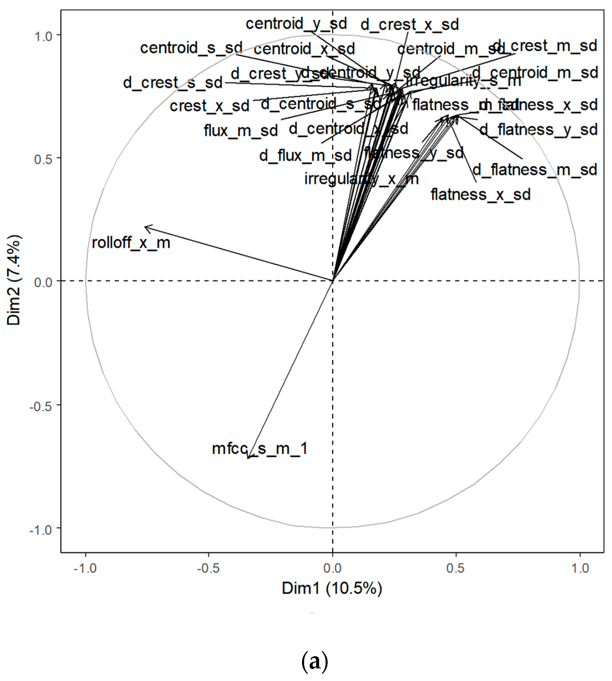
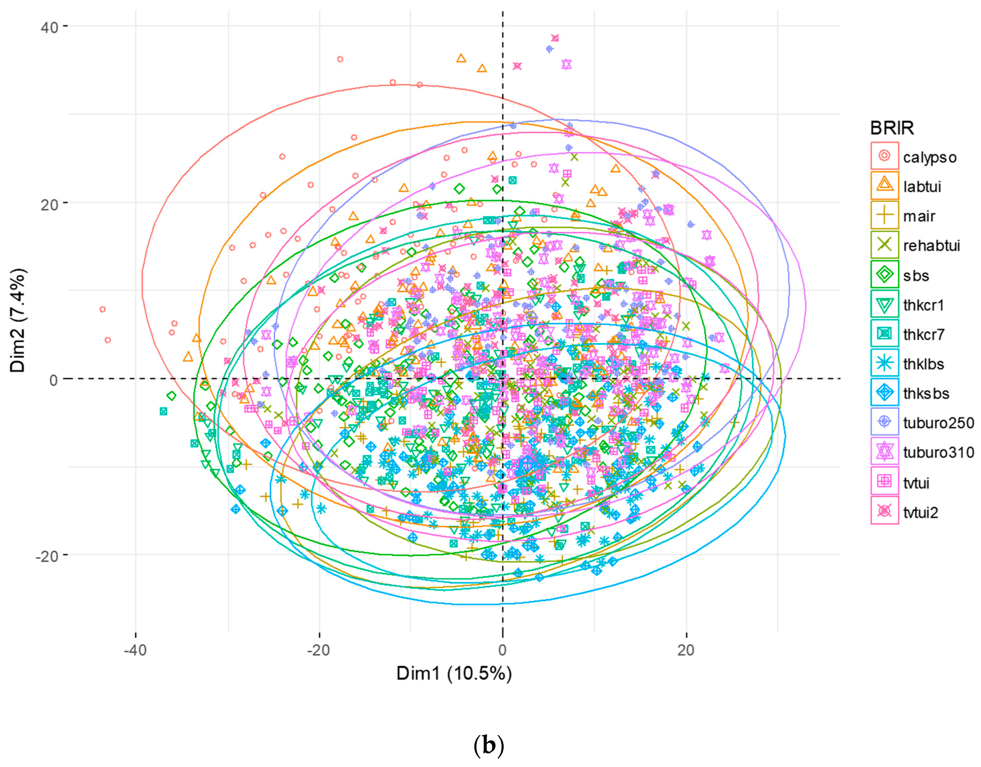
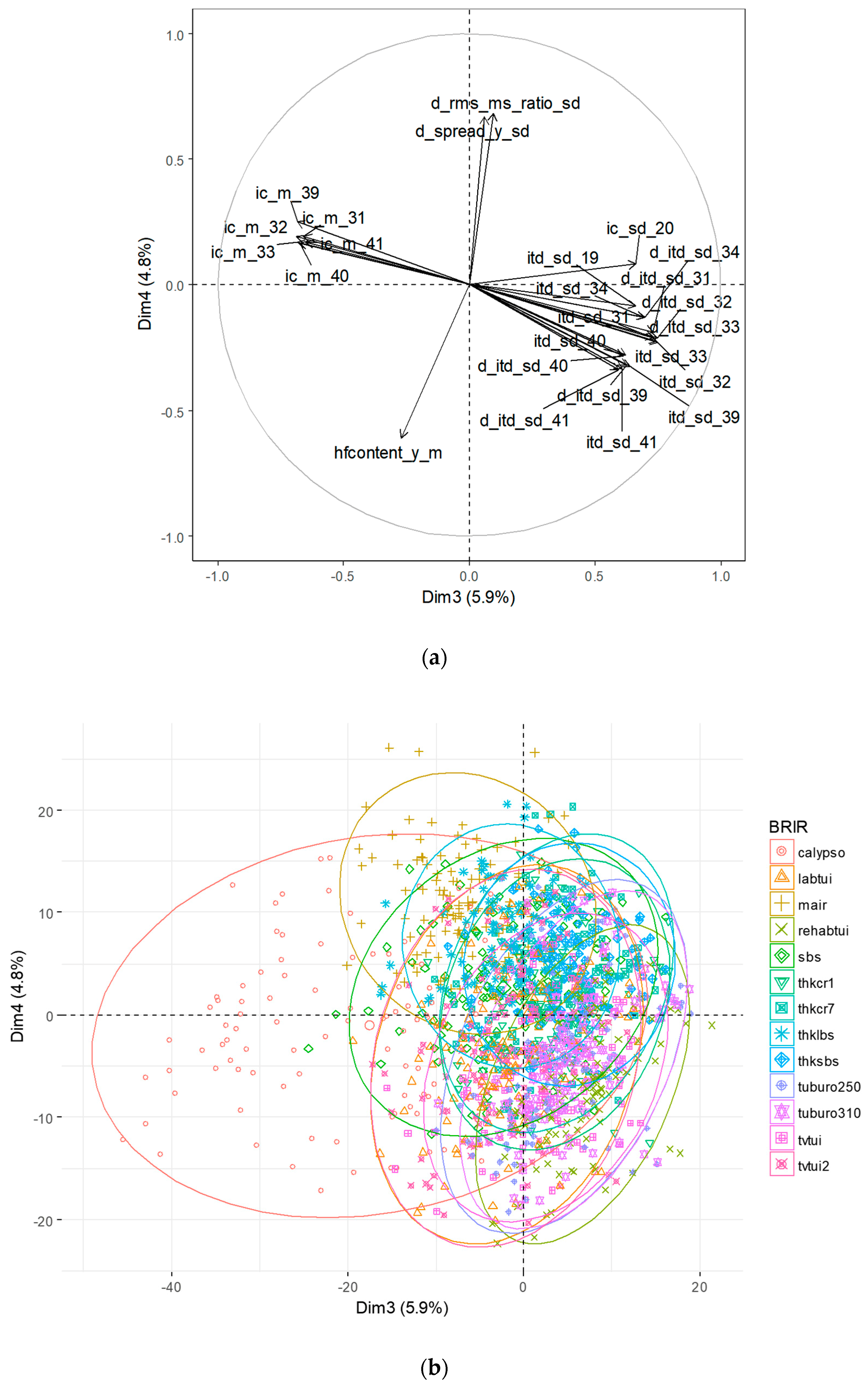
3.3. Principal Component Analysis

In order to further investigate the relations between the BRIR sets, the test dataset was examined using principal component analysis (PCA). According to the Kaiser-Meyer-Olkin overall measure of sampling adequacy (0.8) and Bartlett’s test of sphericity (chi squared tending to infinity, df = 946,000, p = 0), the data were factorizable. The standard PCA method, based on eigenvalue decomposition, was utilized in this study. The obtained results are illustrated in Figure 5 and Figure 6. The first two principal component dimensions accounted for 10.5% and 7.4% of the total variance, respectively. For clarity, the most prominent 25 variables were shown in Figure 5a and Figure 6a. According to Figure 5a, both dimensions predominantly represented the spectral metrics. The first dimension was mainly affected by spectral roll-off, whereas the second dimension was primarily influenced by centroid, crest, flux, and flatness. According to Figure 5b, the stimuli synthesized using all BRIR sets were similar to each other (significant overlap of the BRIR scores).
Principal component dimensions 3 and 4 accounted for 5.9% and 4.8% of the total variance, respectively (Figure 6a). In contrast to the previously discussed results, the calypso BRIR set appeared to be distinctively different compared to the remaining BRIR sets (Figure 6b). This difference was caused by the spatial characteristics of that BRIR set, since dimension 3 was predominantly affected by the binaural cues, such as IC and ITD. Dimension 4 was mainly affected by the spectral features (high frequency content and spectral spread) and, to an extent, by the RMS-based metric. The above observation, regarding the “outlying” characteristics of the stimuli synthesized using the calypso BRIR set, was in line with the results of the informal listening tests described earlier in Section 2.2.2. This observation could also be used as an additional explanation as to why the stimuli synthesized using the calypso BRIR sets were so difficult to predict using the model trained on the remaining BRIR sets (see Table 8).

4. Discussion

The obtained results confirm that the proposed method is capable of predicting the three spatial audio scenes in the binaural recordings of music with a relatively good accuracy, ranging from 74% to 98% (depending on the BRIR set used to synthesize the recordings). The results could be regarded as satisfactory in view of the fact that the method was tested in the reverberant conditions, with an unknown number of foreground objects, with unknown signal characteristics of audio objects, and in a stationary head scenario. The obtained classification accuracy is comparable to the one reached in the pilot test (84%) undertaken by the present authors [20].
While the intra-BRIR generalizability of the method can be regarded as satisfactory, the inter-BRIR generalizability of the method still needs to be improved. The likely reason for the encountered difficulty in the developing of a generalizable model was due to substantial diversity between the recordings synthesized using various BRIR sets. It is expected that the inter-BRIR generalizability could be improved by incorporating a larger number of BRIR sets. Another way of improving the inter-BRIR generalizability might involve a multiconditional training (e.g., under noisy conditions [6]). It is also hypothesized by the authors that incorporating additional recordings in the audio corpus, synthesized using a broad range of head-related transfer functions, could also improve the performance and generalizability of the proposed method.
According to expectations, the binaural cues proved to be the most prominent features in terms of the classification of the spatial audio scenes in binaural recordings of music. However, the MFCCs emerged to be almost as influential as the binaural cues. This outcome could be regarded as surprising since the MFCCs are commonly assumed to be the spectral descriptors [51], not the spatial ones. This study shows that they can also be used as a carrier of spatial information. A possible explanation of this observation could be linked to the mechanism of human hearing responsible for the front–back discrimination, which is predominantly based on the spectral weighting [16]. Since the MFCCs are particularly effective in describing a spectral envelope, it is hypothesized by the present authors that they capture the pinna-related filter characteristics (peaks and notches in the frequency response) responsible for the front–back discrimination.
Most of the BRIR sets used in this study could be characterized as sparse with regards to their spatial resolution. The “missing” impulse responses were interpolated using a vector-base amplitude-panning algorithm [43]. While this method became a de facto standard in the area of spatial audio research, according to its author the method was valid under the assumption that the room was not very reverberant [43]. This assumption was violated for some of the BRIR sets used in this study, which could have an adverse effect on the developed method, for example, by degrading the generalizability of the proposed method for the BRIR sets exhibiting long reverberation times.
Another limitation of the study, potentially degrading the performance of the proposed method, was related to the acoustic mirroring technique used to generate the missing BRIRs, as explained in detail in Section 2. While such an approach was explicitly recommended by the developers of some of the BRIR repositories [37], it was valid under the assumption that the room was symmetric with respect to the position of the dummy head microphone during the measurements of the BRIRs. Considering the architectural drawings accompanying some of the BRIR sets [37], the above assumption was violated. According to the informal listening tests undertaken by the authors, the departure from the above assumption did not affect the perception of the spatial scenes exhibited by the synthesized binaural audio excerpts. However, one cannot exclude a possibility that some of the effects related to the mirroring technique could have been captured by the extracted features and then “perpetuated” in the developed model.
In the present study, only a single classification method was used (LASSO). It is possible that the incorporation of different classification algorithms, such as support vector machines or extreme boosting machines, could improve the results. Due to its relatively large size, the audio corpus used in the study lends itself to deep learning classification techniques. Optimization of the developed method was left for future work.
According to the informal listening test undertaken by the present authors, it is not always easy to distinguish between the FB, BF, and FF scenes. The above difficulty arises from the fact that head movements were deliberately not incorporated in the study. In their study regarding the resolution of front–back ambiguity in spatial hearing, Wightman and Kistler [60] demonstrated, by means of the formal listening tests, that listeners had difficulty discriminating between front and back sources (a task similar in nature to discrimination between FB and BF scenes) if head movements were restricted.
The main focus of this study was the machine learning-based classification, not comparison with the human-based discrimination of the spatial scenes. Formal listening tests, allowing the authors to compare the results obtained using the “machine listener” and human listeners, as well as to verify the definitions of the spatial scenes, were beyond the scope of the present work. However, they are planned to be included in future work.

5. Conclusions

The aim of the study was to develop a method for automatic classification of the three spatial audio scenes, differing in horizontal distribution of foreground and background audio content around a listener in binaurally rendered recordings of music. For the purpose of the study, audio recordings were synthesized using 13 sets of BRIRs, representing both semi-anechoic and reverberant conditions. The proposed method is assumption-free with regards to the number and characteristics of the audio sources (blind classification). Head movements were not considered in the study. A least absolute shrinkage and selection operator was employed as a classifier. According to the results, the method exhibits a satisfactory classification accuracy when it is trained and then tested on the stimuli synthesized using the same BRIRs (accuracy ranging from 74% to 98%), even in highly reverberant conditions. However, the generalizability of the method needs to be further improved.
In addition to the binaural cues, the MFCCs emerged as the prominent metrics, influencing the accuracy of the classified spatial audio scenes. MFCCs are commonly used by researchers as the spectral descriptors of audio signals. This study demonstrates that the MFCCs also constitute a carrier of spatial information. A possible explanation of this observation could be linked to the mechanism of human hearing. Since the MFCCs are particularly effective in describing a spectral envelope of audio signals, it is hypothesized by the present authors that they capture the pinna-related frequency response, responsible for the front–back discrimination of spatial audio stimuli. Further research would be required to validate this hypothesis.

Author Contributions

S.K.Z. developed the concepts and algorithms, carried out the experiments, and wrote the paper. H.L. provided input throughout the development process, undertook the informal listening tests, and provided help with paper writing.

Acknowledgments

This work was partially supported by a grant S/WI/3/2018 from Białystok University of Technology and funded from the resources for research by Ministry of Science and Higher Education in Poland.

Conflicts of Interest

The authors declare no conflict of interest.

References

  1. Kelion, L. YouTube Live-Streams in Virtual Reality and Adds 3D Sound, BBC News. Available online: http://www.bbc.com/news/technology-36073009 (accessed on 18 April 2016).
  2. Parnell, T. Binaural Audio at the BBC Proms. Available online: https://www.bbc.co.uk/rd/blog/2016-09-binaural-proms (accessed on 14 July 2017).
  3. Omnitone: Spatial Audio on the Web, Google, USA. Available online: https://opensource.googleblog.com/2016/07/omnitone-spatial-audio-on-web.html (accessed on 25 July 2016).
  4. Blauert, J. The Technology of Binaural Listening; Springer: Berlin, Germany, 2013. [Google Scholar]
  5. Rumsey, F. Spatial quality evaluation for reproduced sound: Terminology, meaning, and a scene-based paradigm. J. Audio Eng. Soc. 2002, 50, 651–666. [Google Scholar]
  6. May, T.; Ma, N.; Brown, G.J. Robust localisation of multiple speakers exploiting head movements and multi-conditional training of binaural cues. In Proceedings of the IEEE International Conference on Acoustics, Speech and Signal Processing (ICASSP), Brisbane, Australia, 19–24 April 2015. [Google Scholar]
  7. Ma, N.; Brown, G.J. Speech localisation in a multitalker mixture by humans and machines. In Proceedings of the INTERSPEECH 2016, San Francisco, CA, USA, 8–12 September 2016. [Google Scholar]
  8. Ma, N.; Gonzalez, J.A.; Brown, G.J. Robust Binaural Localization of a Target Sound Source by Combining Spectral Source Models and Deep Neural Networks. IEEE/ACM Trans. Audio Speech Lang. Process 2018, 26, 2122–2131. [Google Scholar] [CrossRef]
  9. Benaroya, E.L.; Obin, N.; Liuni, M.; Roebel, A.; Raumel, W.; Argentieri, S. Binaural Localization of Multiple Sound Sources by Non-Negative Tensor Factorization. IEEE/ACM Trans. Audio Speech Lang. Process 2018, 26, 1072–1082. [Google Scholar] [CrossRef] [Green Version]
  10. Lovedee-Turner, M.; Murphy, D. Application of Machine Learning for the Spatial Analysis of Binaural Room Impulse Responses. Appl. Sci. 2018, 8, 105. [Google Scholar] [CrossRef]
  11. Jeffress, L.A. A place theory of sound localization. J. Comp. Physiol. Psychol. 1948, 41, 35–39. [Google Scholar] [CrossRef] [PubMed]
  12. Breebaart, J.; van de Par, S.; Kohlrausch, A. Binaural processing model based on contralateral inhibition. I. Model structure. J. Acoust. Soc. Am. 2001, 110, 1074–1088. [Google Scholar] [CrossRef]
  13. Han, Y.; Park, J.; Lee, K. Convolutional neural networks with binaural representations and background subtraction for acoustic scene classification. In Proceedings of the Conference on Detection and Classification of Acoustic Scenes and Events 2017, Munich, Germany, 16 November 2017. [Google Scholar]
  14. Blauert, J. Spatial Hearing. The Psychology of Human Sound Localization; The MIT Press: London, UK, 1974. [Google Scholar]
  15. Käsbach, J.; Marschall, M.; Epp, B.; Dau, T. The relation between perceived apparent source width and interaural cross-correlation in sound reproduction spaces with low reverberation. In Proceedings of the DAGA 2013, Merano, Italy, 18–21 March 2013. [Google Scholar]
  16. Zonoz, B.; Arani, E.; Körding, K.P.; Aalbers, P.A.T.R.; Celikel, T.; Van Opstal, A.J. Spectral Weighting Underlies Perceived Sound Elevation. Nat. Sci. Rep. 2019, 9, 1–12. [Google Scholar] [CrossRef] [PubMed]
  17. Raake, A. A Computational Framework for Modelling Active Exploratory Listening that Assigns Meaning to Auditory Scenes—Reading the World with Two Ears. Available online: http://twoears.eu (accessed on 8 March 2019).
  18. Ibrahim, K.M.; Allam, M. Primary-ambient source separation for upmixing to surround sound systems. In Proceedings of the IEEE International Conference on Acoustics, Speech and Signal Processing (ICASSP), Calgary, Canada, 15–20 April 2018. [Google Scholar]
  19. Hummersone, C.H.; Mason, R.; Brookes, T. Dynamic Precedence Effect Modeling for Source Separation in Reverberant Environments. IEEE Trans. Audio Speech Lang. Process 2010, 18, 1867–1871. [Google Scholar] [CrossRef] [Green Version]
  20. Zieliński, S.K.; Lee, H. Feature Extraction of Binaural Recordings for Acoustic Scene Classification. In Proceedings of the 2018 Federated Conference on Computer Science and Information Systems (FedCSIS), Poznań, Poland, 9–12 September 2018. [Google Scholar]
  21. Sturm, B.L. A Survey of Evaluation in Music Genre Recognition. In Adaptive Multimedia Retrieval: Semantics, Context, and Adaptation; Lecture Notes in Computer Science; Springer: Cham, Switzerland, 2014. [Google Scholar]
  22. Zieliński, S.; Rumsey, F.; Kassier, R. Development and Initial Validation of a Multichannel Audio Quality Expert System. J. Audio Eng. Soc. 2005, 53, 4–21. [Google Scholar]
  23. Zieliński, S.K. Feature Extraction of Surround Sound Recordings for Acoustic Scene Classification. In Artificial Intelligence and Soft Computing, Proceedings of the ICAISC 2018; Lecture Notes in Computer Science; Springer: Cham, Switzerland, 2018. [Google Scholar]
  24. Zieliński, S.K. Spatial Audio Scene Characterization (SASC). Automatic Classification of Five-Channel Surround Sound Recordings According to the Foreground and Background Content. In Multimedia and Network Information Systems, Proceedings of the MISSI 2018; Advances in Intelligent Systems and Computing; Springer: Cham, Switzerland, 2019. [Google Scholar]
  25. Beresford, K.; Zieliński, S.; Rumsey, F. Listener Opinions of Novel Spatial Audio Scenes. In Proceedings of the 120th AES Convention, Paris, France, 20–23 May 2006. [Google Scholar]
  26. Lee, H.; Millns, C. Microphone Array Impulse Response (MAIR) Library for Spatial Audio Research. In Proceedings of the 143rd AES Convention, New York, NY, USA, 21 October 2017. [Google Scholar]
  27. Zieliński, S.; Rumsey, F.; Bech, S. Effects of Down-Mix Algorithms on Quality of Surround Sound. J. Audio Eng. Soc. 2003, 51, 780–798. [Google Scholar]
  28. Szabó, B.T.; Denham, S.L.; Winkler, I. Computational models of auditory scene analysis: A review. Front. Neurosci. 2016, 10, 1–16. [Google Scholar] [CrossRef]
  29. Alinaghi, A.; Jackson, P.J.B.; Liu, Q.; Wang, W. Joint Mixing Vector and Binaural Model Based Stereo Source Separation. IEEE/ACM Trans. Audio Speech Lang. Process 2014, 22, 1434–1448. [Google Scholar] [CrossRef]
  30. Barchiesi, D.; Giannoulis, D.; Stowell, D.; Plumbley, M.D. Acoustic scene classification: Classifying environments from the sounds they produce. IEEE Signal. Process. Mag. 2015, 32, 16–34. [Google Scholar] [CrossRef]
  31. Pätynen, J.; Pulkki, V.; Lokki, T. Anechoic Recording System for Symphony Orchestra. Acta Acust united Ac. 2008, 94, 856–865. [Google Scholar] [CrossRef]
  32. D’Orazio, D.; De Cesaris, S.; Garai, M. Recordings of Italian opera orchestra and soloists in a silent room. Proc. Mtgs. Acoust. 2016, 28, 015014. [Google Scholar]
  33. Mixing Secrets for The Small Studio. Available online: http://www.cambridge-mt.com/ms-mtk.htm (accessed on 8 March 2019).
  34. Bittner, R.; Salamon, J.; Tierney, M.; Mauch, M.; Cannam, C.; Bello, J.P. MedleyDB: A Multitrack Dataset for Annotation-Intensive MIR Research. In Proceedings of the 15th International Society for Music Information Retrieval Conference, Taipei, Taiwan, 27 October 2014. [Google Scholar]
  35. Studio Sessions. Telefunken Elektroakustik. Available online: https://telefunken-elektroakustik.com/multitracks (accessed on 8 March 2019).
  36. Satongar, D.; Lam, Y.W.; Pike, C.H. Measurement and analysis of a spatially sampled binaural room impulse response dataset. In Proceedings of the 21st International Congress on Sound and Vibration, Beijing, China, 13–17 July 2014. [Google Scholar]
  37. Stade, P.; Bernschütz, B.; Rühl, M. A Spatial Audio Impulse Response Compilation Captured at the WDR Broadcast Studios. In Proceedings of the 27th Tonmeistertagung—VDT International Convention, Cologne, Germany, 20 November 2012. [Google Scholar]
  38. Wierstorf, H. Binaural Room Impulse Responses of a 5.0 Surround Setup for Different Listening Positions. Zenodo. Available online: https://zenodo.org (accessed on 14 October 2016).
  39. Lee, H. Sound Source and Loudspeaker Base Angle Dependency of Phantom Image Elevation Effect. J. Audio Eng. Soc. 2017, 65, 733–748. [Google Scholar] [CrossRef] [Green Version]
  40. Werner, S.; Voigt, M.; Klein, F. Dataset of Measured Binaural Room Impulse Responses for Use in an Position-Dynamic Auditory Augmented Reality Application. Zenodo. Available online: https://zenodo.org (accessed on 26 July 2018).
  41. Klein, F.; Werner, S.; Chilian, A.; Gadyuchko, M. Dataset of In-The-Ear and Behind-The-Ear Binaural Room Impulse Responses used for Spatial Listening with Hearing Implants. In Proceedings of the 142nd AES Convention, Berlin, Germany, 20–23 May 2017. [Google Scholar]
  42. Erbes, V.; Geier, M.; Weinzierl, S.; Spors, S. Database of single-channel and binaural room impulse responses of a 64-channel loudspeaker array. In Proceedings of the 138th AES Convention, Warsaw, Poland, 7–10 May 2015. [Google Scholar]
  43. Pulkki, V. Virtual Sound Source Positioning Using Vector Base Amplitude Panning. J. Audio Eng. Soc. 1997, 45, 456–466. [Google Scholar]
  44. Politis, A. Vector-Base Amplitude Panning Library. Available online: https://github.com (accessed on 1 January 2015).
  45. Wierstorf, H.; Spors, S. Sound Field Synthesis Toolbox. In Proceedings of the 132nd AES Convention, Budapest, Hungary, 26–29 April 2012. [Google Scholar]
  46. Rabiner, L.; Juang, B.-H.; Yegnanarayana, B. Fundamentals of Speech Recognition; Pearson India: New Delhi, India, 2008. [Google Scholar]
  47. Dau, T.; Püschel, D.; Kohlrausch, A. A quantitative model of the “effective” signal processing in the auditory system. I. Model structure. J. Acoust. Soc. Am. 1996, 99, 3615. [Google Scholar] [CrossRef]
  48. Brown, G.J.; Cooke, M. Computational auditory scene analysis. Comput. Speech Lang. 1994, 8, 297–336. [Google Scholar] [CrossRef]
  49. George, S.; Zieliński, S.; Rumsey, F.; Jackson, P.; Conetta, R.; Dewhirst, M.; Meares, D.; Bech, S. Development and Validation of an Unintrusive Model for Predicting the Sensation of Envelopment Arising from Surround Sound Recordings. J. Audio Eng. Soc. 2010, 58, 1013–1031. [Google Scholar]
  50. Conetta, R.; Brookes, T.; Rumsey, F.; Zieliński, S.; Dewhirst, M.; Jackson, P.; Bech, S.; Meares, D.; George, S. Spatial audio quality perception (part 2): A linear regression model. J. Audio Eng. Soc. 2014, 62, 847–860. [Google Scholar] [CrossRef]
  51. Lerch, A. An Introduction to Audio Content Analysis Applications in Signal. Processing and Music Informatics; IEEE Press: Berlin, Germany, 2012. [Google Scholar]
  52. Peeters, G.; Giordano, B.; Susini, P.; Misdariis, N.; McAdams, S. Extracting audio descriptors from musical signals. J. Acoust. Soc. Am. 2011, 130, 2902–2916. [Google Scholar] [CrossRef]
  53. Jensen, K.; Andersen, T.H. Real-time beat estimation using feature extraction. In Computer Music Modeling and Retrieval; Lecture Notes in Computer Science; Springer: Berlin, Germany, 2004. [Google Scholar]
  54. Scheirer, E.; Slaney, M. Construction and evaluation of a robust multifeature speech/music discriminator. In Proceedings of the IEEE International Conference on Acoustics, Speech, and Signal Processing, Munich, Germany, 21–24 April 1997. [Google Scholar]
  55. McCree, A.; Sell, G.; Garcia-Romero, D. Extended Variability Modeling and Unsupervised Adaptation for PLDA Speaker Recognition. In Proceedings of the INTERSPEECH 2017, Stockholm, Sweden, 20–24 August 2017. [Google Scholar]
  56. Shen, Z.; Yong, B.; Zhang, G.; Zhou, R.; Zhou, Q. A Deep Learning Method for Chinese Singer Identification. Tsinghua Sci. Technol. 2019, 24, 371–378. [Google Scholar] [CrossRef]
  57. Dormann, C.F.; Elith, J.; Bacher, S.; Buchmann, C.; Carl, G.; Carré, G.; Marquéz, J.R.G.; Gruber, B.; Lafourcade, B.; Leitão, P.J.; et al. Collinearity: A review of methods to deal with it and a simulation study evaluating their performance. Ecography 2012, 36, 27–46. [Google Scholar] [CrossRef]
  58. James, G.; Witten, D.; Hastie, T.; Tibshirani, R. An Introduction to Statistical Learning with Applications in R; Springer: London, UK, 2017. [Google Scholar]
  59. Kuhn, M. The Caret Package. Available online: https://topepo.github.io/caret (accessed on 26 May 2018).
  60. Wightman, F.; Kistler, D. Resolution of Front–Back Ambiguity in Spatial Hearing by Listener and Source Movement. J. Acoust. Soc. Am. 1999, 105, 2841–2853. [Google Scholar] [CrossRef]
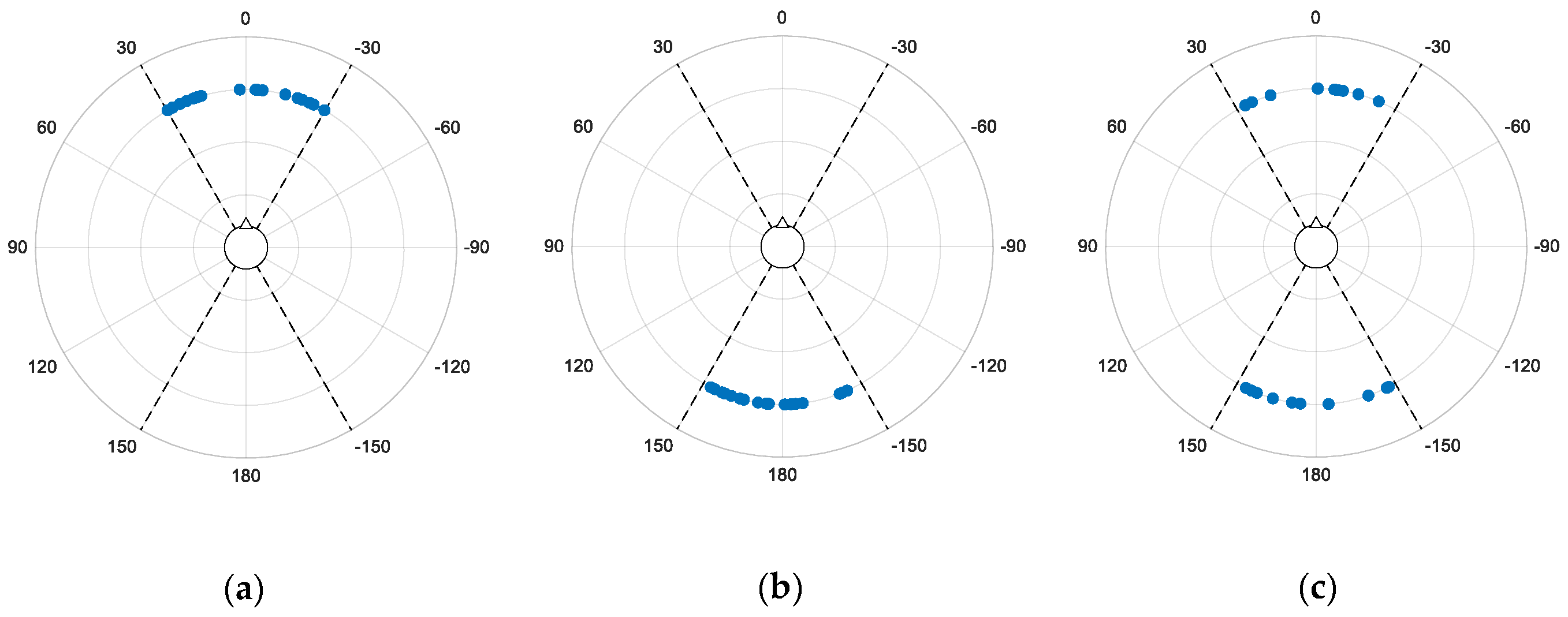
Figure 1. Block diagram of the basic spatial audio scene classifier (output categories are explained in the text). FB: foreground–background; BF: background–foreground; FF: foreground–foreground.
Applsci 09 01724 g001
Figure 2. Examples of an intended placement of 20 foreground audio objects for: (a) FB scene; (b) BF scene; (c) FF scene.
Applsci 09 01724 g002
Figure 3. Confusion matrices obtained for the models trained and tested using recordings synthesized with selected sets of BRIRs: (a) all BRIR sets; (b) sbs; (c) mair; (d) calypso; (e) tuburo250; and (f) tuburo310.
Applsci 09 01724 g003
Figure 4. Confusion matrices obtained for the best three models in experiment 2: (a) tvtui2; (b) tuburo310; and (c) labtui.
Applsci 09 01724 g004
Figure 5. Results of the principle component analysis (PCA) for dimensions 1 and 2: (a) variable plot; (b) audio recordings. Ellipses represent a concentration of the scores for each BRIR set with 95% confidence boundaries around group means.
Applsci 09 01724 g005aApplsci 09 01724 g005b
Figure 6. Results of the PCA for dimensions 3 and 4: (a) variable plot; (b) audio recordings. Ellipses represent a concentration of the scores for each BRIR set with 95% confidence boundaries around group means.
Applsci 09 01724 g006
Table 1. The basic spatial audio scenes.
Acoustic SceneDescription
Foreground–Background (FB)A listener perceives foreground audio content in the front and background content behind the head.
Background–Foreground (BF)A listener perceives background audio content in the front and foreground content behind the head.
Foreground–Foreground (FF)A listener is surrounded by foreground audio content.
Table 2. Overview of the binaural-room-impulse-response (BRIR) sets used in the study.
No.AcronymDescriptionDummy HeadRT60 (s)
1sbsSalford, British Broadcasting Corporation (BBC)–Listening Room [36]B&K HATS Type 41000.27
2mairHuddersfield–Concert Hall [26]Neumann KU1002.1
3thkcr1Westdeutscher Rundfunk (WDR) Broadcast Studios–Control Room 1 [37]Neumann KU1000.23
4thkcr7WDR Broadcast Studios–Control Room 7 [37]Neumann KU1000.27
5thksbsWDR Broadcast Studios–Small Broadcast Studio (SBS) [37]Neumann KU1001.0
6thklbsWDR Broadcast Studios–Large Broadcast Studio (LBS) [37]Neumann KU1001.8
7calypsoTechnische Universität (TU) Berlin–Calypso Room [38]KEMAR 45BA0.17
8tvtuiTU Ilmenau–TV Studio (distance of 3.5m) [40]KEMAR 45BA0.7
9tvtui2TU Ilmenau–TV Studio (distance of 2m) [41]KEMAR 45BA0.7
10labtuiTU Ilmenau–Listening Laboratory [41]KEMAR 45BA0.3
11rehabtuiTU Ilmenau–Rehabilitation Laboratory [41]KEMAR 45BANA
12tuburo250University of Rostock–Audio Laboratory (additional absorbers) [42]KEMAR 45BA0.25
13tuburo310University of Rostock–Audio Laboratory (all broadband absorbers) [42]KEMAR 45BA0.31
Table 3. Overview of the extracted features (1376 metrics in total).
Spatial FeaturesSpectro-Temporal Features
Feature AcronymRoot Mean Square (RMS)Binaural CuesSpectral FeaturesMel-Frequency Cepstral Coefficient (MFCC)
Number of Features8504224640
Table 4. Accuracy of classification (%) obtained upon training and testing of the model. The training and testing repository consisted of 4368 and 1560 audio excerpts, respectively.
DatasetRMSBinauralMFCCSpectralRMS + BinauralMFCC + SpectralAll Features
Training38.272.974.950.073.175.181.2
Testing39.973.169.052.273.667.876.9
Table 5. Training accuracy (%) of the models obtained using subsets of recordings synthesized with individual BRIR sets. Each training subset included 336 audio excerpts.
IDBRIRRMSBinauralMFCCSpectralRMS + BinauralMFCC + SpectralAll Features
1sbs43.991.588.549.591.588.091.7
2mair48.591.885.951.691.884.992.2
3thkcr146.396.882.142.196.881.696.2
4thkcr737.994.884.248.294.983.894.7
5thksbs35.987.972.542.587.972.487.6
6thklbs50.285.468.847.785.368.185.7
7calypso69.397.595.282.797.595.697.8
8tvtui48.388.674.058.788.673.887.7
9tvtui245.685.380.247.285.179.986.9
10labtui40.779.171.244.679.470.478.9
11rehabtui46.384.273.444.684.372.485.4
12tuburo25038.366.772.258.666.772.071.0
13tuburo31040.466.271.556.966.670.673.6
Table 6. Testing accuracy (%) of the models obtained using subsets of recordings synthesized with individual BRIR sets. Each testing subset consisted of 120 audio excerpts.
IDBRIRRMSBinauralMFCCSpectralRMS + BinauralMFCC + SpectralAll Features
1sbs50.895.893.356.795.893.397.5
2mair54.294.284.247.594.281.795.8
3thkcr150.898.385.045.898.383.398.3
4thkcr737.595.890.860.095.891.796.7
5thksbs42.584.275.048.384.275.084.2
6thklbs50.885.873.353.385.875.085.8
7calypso69.297.597.575.897.597.596.7
8tvtui50.885.072.561.785.073.386.7
9tvtui246.789.278.353.390.076.790.8
10labtui40.879.283.345.878.385.084.2
11rehabtui40.881.779.240.881.778.388.3
12tuburo25043.365.080.855.865.081.780.8
13tuburo31035.870.875.052.570.875.074.2
Table 7. Accuracy of classification (%) obtained for models trained and tested using the recordings synthesized with BRIR sets of similar reverberation time. Numbers in brackets represent 95% confidence intervals.
Reverberation TimeRT60BRIRs Used for TrainingBRIRs Used for TestingTest Accuracy (%)
Short0.17−0.31 ssbs, thkcr1, calypso, labtui, tuburo310thkcr7, tuburo25065.4 (59.0, 71.4)
Medium0.7−1.0 sthksbs, tvtuitvtui251.7 (42.4, 60.9)
Long1.8−2.1 sthklbsmair40.0 (31.2, 49.3)
Table 8. The results of the leave-one-BRIR-out validation. Numbers in brackets represent 95% confidence intervals.
No.BRIR Set Left-OutTraining Accuracy (%)Testing Accuracy (%)
1sbs80.844.2 (35.1, 53.5)
2mair80.856.7 (47.3, 65.7)
3thkcr181.545.8 (36.7, 55.2)
4thkcr780.665.0 (55.8, 73.5)
5thksbs81.165.0 (55.8, 73.5)
6thklbs82.050.0 (40.7, 59.3)
7calypso80.637.5 (28.8, 46.8)
8tvtui80.855.8 (46.5, 64.9)
9tvtui281.179.2 (70.8, 86.0)
10labtui81.765.8 (56.6, 74.2)
11rehabtui81.935.8 (27.3, 45.1)
12tuburo25081.664.2 (54.9, 72.7)
13tuburo31081.073.3 (64.5, 81.0)

