Article

Particle Swarm Optimization and Cuckoo Search-Based Approaches for Quadrotor Control and Trajectory Tracking

1
Faculty of Science and Technology, Cadi Ayyad University, Marrakesh 40000, Morocco
2
Royal School of Aeronautics, Marrakesh 40000, Morocco
*
Author to whom correspondence should be addressed.
Appl. Sci. 2019, 9(8), 1719; https://doi.org/10.3390/app9081719
Submission received: 19 March 2019 / Revised: 17 April 2019 / Accepted: 17 April 2019 / Published: 25 April 2019
(This article belongs to the Special Issue Applied Sciences Based on and Related to Computer and Control)

Abstract

:
This paper explores the full control of a quadrotor Unmanned Aerial Vehicles (UAVs) by exploiting the nature-inspired algorithms of Particle Swarm Optimization (PSO), Cuckoo Search (CS), and the cooperative Particle Swarm Optimization-Cuckoo Search (PSO-CS). The proposed PSO-CS algorithm combines the ability of social thinking in PSO with the local search capability in CS, which helps to overcome the problem of low convergence speed of CS. First, the quadrotor dynamic modeling is defined using Newton-Euler formalism. Second, PID (Proportional, Integral, and Derivative) controllers are optimized by using the intelligent proposed approaches and the classical method of Reference Model (RM) for quadrotor full control. Finally, simulation results prove that PSO and PSO-CS are more efficient in tuning of optimal parameters for the quadrotor control. Indeed, the ability of PSO and PSO-CS to track the imposed trajectories is well seen from 3D path tracking simulations and even in presence of wind disturbances.

1. Introduction

Over the past few years, Unmanned Aerial Vehicles (UAVs) of type quadrotors or quadcopters have seen an increasing interest since their wide range of civilian and military applications. These quadrotors are considered the most complex flying machines due to many physical effects influencing their dynamics including aerodynamic effects, gravity, gyroscopic effects, friction, and inertia. However, they have advantages over conventional helicopters. Given that the left and the right motors rotate clockwise, and the front and the rear motors rotate counterclockwise, gyroscopic effects and aerodynamic torques tend to cancel in trimmed flight.
Many researchers modeled the quadrotor using the formalisms of Newton-Euler [1,2] and Euler-Lagrange [2,3,4]. For both methods, the quadrotor modeling is regarded as a delicate task and the model obtained using these approaches is strongly nonlinear, fully coupled, under-actuated (Six Degrees of Freedom System (6-DOF) with only four actuators) and dynamically unstable with complex behavior. In this work, we adopt the most used formalism of Newton-Euler to define the dynamics of the quadrotor.
Regarding the quadrotor’s control, there are several types of research done both in linear and nonlinear control methods [5,6,7]. For practicality, the linear controllers, especially PID (Proportional, Integral, and Derivative)/PD (Proportional and Derivative)/ PI (Proportional and Integral), are easy to design and simple to tune, which perform better in practical implementation [8]. In literature, PIDs are the most used for quadrotor control [2,9,10]. However, tuning the parameters of these controllers is very important to get best performances. In this scope, classical methods can be used. They include the methods of Ziegler-Nichols [11], Graham-Lathrop [12], Naslin [13], Cohen-Coon, Reference Model (RM) [14,15], and many other techniques.
Nature-inspired optimization algorithms can effectively resolve complex problems compared to classical and statistical methods. Some of these algorithms proposed in the literature are Genetic Algorithm (GA) [16,17], Particle Swarm Optimization (PSO) [18], Ant Colony Optimization (ACO) [19], Artificial Bee Colony (ABC) [20], and Cuckoo Search (CS) [21,22]. GA is inspired by the crossover, mutation, and recombination principles of genetics. PSO algorithm is inspired by social behavior patterns of organisms that live and interact within large groups. It incorporates swarming behaviors observed in flocks of birds and schools of fish. ACO is inspired by ants’ behavior in seeking food sources. The ABC algorithm is based on the natural behavior of honeybee swarm, and CS algorithm is motivated by the aggressive breeding of a bird called ‘cuckoo’. The PSO method has shown superior performances. It has features such as a straightforward algorithm, rapid convergence, easy implementation, and is computationally efficient when applied to a diverse set of optimization problems [15]. In CS, immigration and environmental specifications have the advantage to help cuckoos’ groups to converge and reach the best places for breeding and egg laying [21]. Another advantage of CS compared to PSO and GA is that it uses a smaller number of parameters to be tuned, which makes it more adaptable [21]. Due to these advantages, PSO and CS are still successfully applied in recent works for control problems [23,24,25], and PSO is especially used in tuning PID controllers for quadrotor’s control [26,27]. Therefore, regarding PSO and CS programs, there are many common points. Both use the same initialization matrices of particles in n-dimensional research space for PSO and nests with D eggs (problem’s dimension) for CS. The fitness function evaluates the quality of particles and nests in the same way. Then, the velocities of displacement of particles and nests are calculated in different ways for PSO and CS, which generates differences in the convergence speeds of both algorithms. For these reasons, it would be very interesting to analyze the social thinking and local search abilities of PSO and CS in quadrotor control.
The main contribution of our paper lies on using PSO and CS to improve results concerning the quadrotor full control. However, the CS algorithm suffers from a low convergence speed, since it uses a fixed step size over generations. To overcome this problem, Naik et al. [28] proposed an adaptive cuckoo search algorithm (ACS) with adaptive step size. The ACS converges to a near optimum solution faster than CS algorithm. However, the problem of ACS algorithm is that it does not achieve better solutions compared to CS in most cases. In our work, we propose the cooperative PSO-CS algorithm that combines the ability of social thinking in PSO with the local search capability of CS. Such a cooperative process is likely to offer proper guidance for cuckoos to the global best positions and to ensure a balance between exploitation and exploration of the search space. Consequently, we are interested in examining if it is possible for us to improve results of quadrotor control by effectively integrating these two algorithms with complementary strengths. Our work treats position and attitude control in order to cover all topics in quadrotor control. For this objective, the control design includes six PID controllers: Three for angles (ϕ, θ, ψ) and three for positions (x, y, z). These controllers are optimally tuned using the heuristics PSO and CS, the cooperative PSO-CS and the classical method of Reference Model (RM). A comparative study is done to highlight the efficiency of the proposed intelligent controllers of PSO and PSO-CS. Indeed, their robustness is demonstrated in presence of wind disturbance.
The rest of this paper is organized as follows. In Section 2, Newton-Euler formalism is used to establish the quadrotor dynamic model. In Section 3, the proposed algorithms of PSO, CS, the cooperative PSO-CS and RM are presented. In Section 4, the quadrotor full control is treated using PID controllers optimally tuned with the proposed methods. In the last section, our conclusions are given.

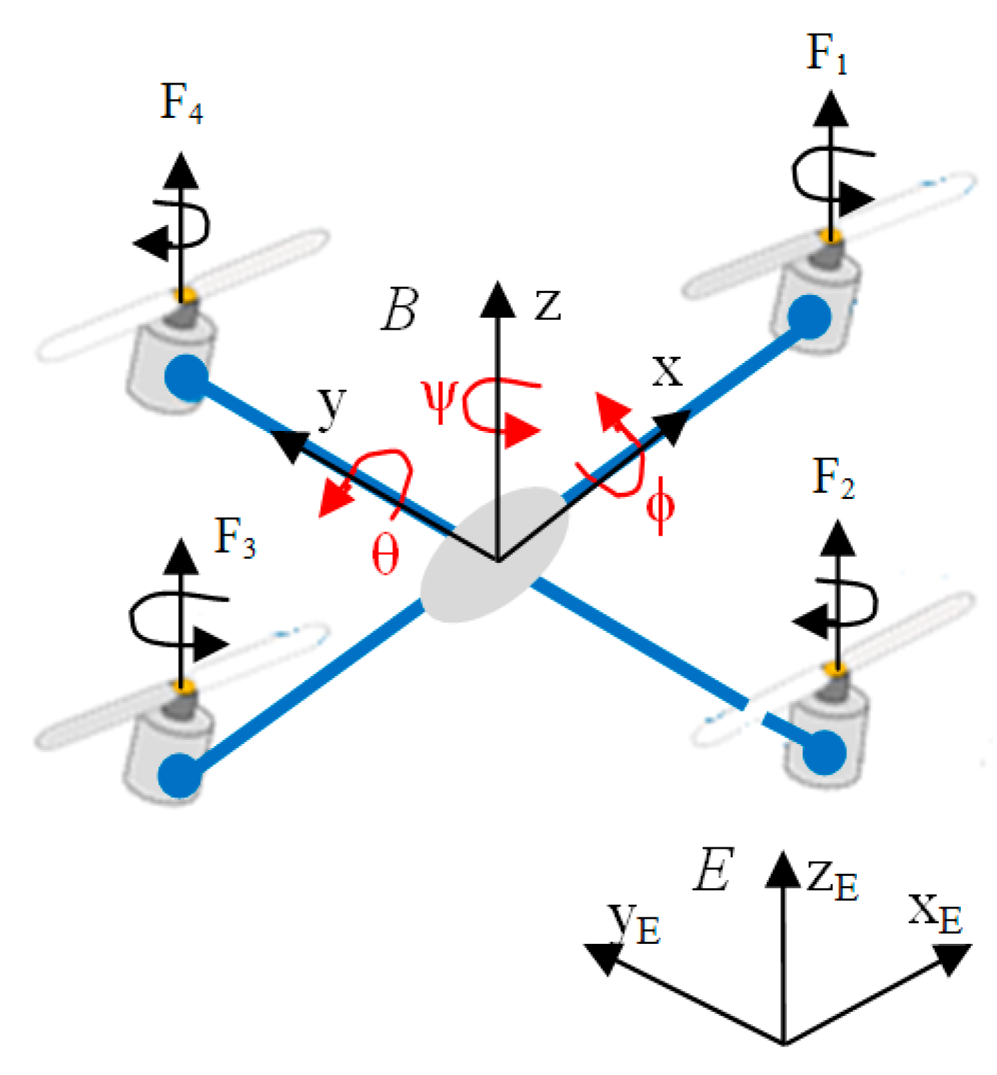
2. Quadrotor Dynamic Modeling

The quadrotor is a complex flying system, strongly nonlinear, multivariable, fully coupled, and under-actuated (6-DOF and only four control inputs). Therefore, its modeling is a delicate task. For better understanding of its dynamic modeling, different working hypotheses were assumed: A rigid and a symmetrical quadrotor structure (diagonal matrix of inertia); a rigid propellers (negligible effect of deformation during rotation); the lift and the drag forces are proportional to the square of the rotational speed of the rotors (a very close approximation of the aerodynamic behavior); and the center of mass is exactly the origin of reference related to the structure.
From the configuration shown in Figure 1, the quadrotor has two pairs of rotating rotors attached to the end of a cross and the control electronics is situated in the center of the cross. The front and the rear propellers spin counterclockwise, while the left and the right ones spin clockwise, which effectively neutralizes the unwanted reactive torque and allows the vehicle to fly without overturning.
Notice that the absolute position of the mass center is described by the three coordinates (x, y, z) and its attitude by the three Euler’s angles (ϕ, θ, ψ). Using Newton-Euler formalism [2], the dynamic model of the quadrotor can be expressed as:
φ ¨ = l   U 2 I x + ( I y I z ) I x ( ψ   ˙ c o s φ   c o s θ θ ˙ s i n φ ) ( θ ˙ c o s φ + ψ ˙   s i n φ   c o s θ )         J r ( ω 1 ω 2 + ω 3 ω 4 ) I x ( ψ   ˙ s i n φ   c o s θ + θ ˙   c o s φ )         K f a x I x ( φ ˙ 2 2 φ ˙ ψ   ˙ s i n θ 2 )
θ ¨ = l   U 3 I y + ( I z I x ) I y ( ψ ˙   c o s φ   c o s θ θ   ˙ s i n φ ) ( φ ˙ ψ   ˙ s i n θ )         J r ( ω 1 ω 2 + ω 3 ω 4 ) I y ( ψ   ˙ s i n θ ϕ ˙ )         K f a y I y ( θ ˙ 2   c o s φ 2 + 2 φ ˙   ψ ˙   s i n φ   c o s φ   c o s θ   + ψ ˙ 2   s i n φ 2   c o s θ 2 )
ψ ¨ = U 4 I z + ( I x I y ) I z ( ψ   ˙ s i n φ   c o s θ + θ ˙   c o s φ ) ( φ ˙ ψ   ˙ s i n θ )         J r ( ω 1 ω 2 + ω 3 ω 4 ) I y ( ψ ˙   s i n θ φ ˙ ) ( θ ˙ 2 s i n φ 2         2 φ ˙ ψ ˙   s i n φ   c o s φ   c o s θ ) + K f a z I z ψ ˙ 2 c o s φ 2 c o s θ 2
x ¨ = cos φ   cos φ   sin θ + sin φ   sin ψ m U 1 K f t x m x ˙
y ¨ = sin ψ   sin θ   cos φ cos ψ   sin φ m U 1 K f t y m y ˙
z ¨ = g + cos φ cos θ m U 1 K f t z m z ˙
with
{ U 1 = b ( ω 1 2 + ω 2 2 + ω 3 2 + ω 4 2 ) U 2 = b ( ω 4 2 ω 2 2 ) U 3 = b ( ω 3 2 ω 1 2 ) U 4 = d ( ω 1 2 ω 2 2 + ω 3 2 ω 4 2 )
where m is the total mass of the quadrotor; l the distance from the center of the body to the rotor; Ix, Iy and Iz are the inertias around x, y, and z axis; b and d thrust and drag coefficients respectively; Kfax, Kfay, and Kfaz are frictions aerodynamics coefficients; Kftx, Kfty, and Kftz are translation drags coefficients; Jr is the rotor inertia; g represents gravity constant; ωi is the angular speed of the motor i and finally ϕ, θ, and ψ are rotation around the roll, pitch, and yaw axis, respectively.

3. Proposed Methods

Intelligent and classical control methods of Particle Swarm Optimization (PSO), Cuckoo Search (CS), the cooperative PSO-CS, and the classical Reference Model (RM) are detailed in this section for further reason to be applied in quadrotor control.

3.1. PSO Algorithm

Particle Swarm Optimization (PSO) is a class of stochastic algorithms, which was developed by Eberhart and Kennedy in 1995 for hard optimization problems. The basic principle of PSO is inspired by the social behavior of animals moving in swarm as bird flocking. To search for food, each bird called particle, flies in the space of solutions, and determines its speed according to its personal experience and the information gained through interaction with other swarm members [18].
PSO is employed to intelligently select optimal parameters from N particles. The initialization matrix contains N particles dispersed in a D-dimensional search space. Like most optimization techniques, PSO requires a fitness function relevant to the particle’s position. Each particle i stores its best position Pbi(t+1) and the best solution in its vicinity Pg(t+1), which is the position of the particle that has the smallest fitness value in the swarm as expressed in Equation (9). The mechanism of displacement of each particle is managed by three rules. First, the particle tends to follow the direction of its current velocity. Second, it wants to move toward its best position. Finally, it tends to move to the best position reached by its neighbors [18,29]. In fact, the new velocity matrix Vij and position matrix Xij of the particle i = {1, 2, …, N} in the search space of dimension D, with j = {1, 2, …, D} are calculated at iteration (t+1), according to Equations (10) and (11).
P b i ( t + 1 ) = { X i ( t + 1 ) i f       f ( X i ( t + 1 ) ) < f ( P b i ( t ) ) P b i ( t ) e l s e
P g = m i n i = 1 , 2 N f ( P b i ( t + 1 ) )
V i j ( t + 1 ) = w V i j ( t ) + R 1 C 1 ( P b i j ( t ) X i j ( t ) ) + R 2 C 2 ( P g i j ( t ) X i j ( t ) )
X i j ( t + 1 ) = X i j ( t ) + V i j ( t + 1 )
where
  • Pbij is the best position found by the particle i;
  • Pgij is the best position found by the neighborhood;
  • w, C1, and C2 are weighting coefficients;
  • R1 and R2 are random variables generated from a uniform distribution in [0,1];
  • ⊗ means element wise multiplications.
The weighting coefficients govern the process of finding the best solution and reflect the sociability of the particles. In order to move the particle towards the best solutions, selection of these coefficients must ensure a compromise between local and global exploration of the search space. In previous works [30,31], the constants C1 and C2 must verify the condition C1 + C2 ≤ 4. Also, experimental results in Reference [30] show that [1/2((C1 + C2) − 1)] < w ≤ 1. PSO search works in G iterations and the coordinates of the obtained global best position Pg are the parameters optimally tuned.

3.2. CS Algorithm

Cuckoo Search (CS) algorithm, proposed by Yang and Deb in 2009, is based on the life of the ”cuckoo” bird. The basic principle of this optimization algorithm is the specific breeding and egg laying of this bird. In the habitat of other host birds, adult cuckoos lay some eggs that grow and become mature cuckoos if they are not discovered and removed by host birds. The immigration of groups of cuckoos and environmental specifications hopefully lead them to converge and reach the best places for reproduction and breeding [21].
The primary population of CS is composed of N nests representing a set of solutions, where each nest has multiple eggs (D eggs). As in nature, each cuckoo dedicates from five to 20 eggs. These values are used as the limits of the dimension D. Each cuckoo lays one egg at a time and dumps it in a randomly chosen nest. The best nests with high-quality eggs (solutions) will carry over to the next generations, where the profit of a solution is obtained by evaluation of a fitness function F of the habitat, so the profit is an array of 1 × D. The number of available host nests is fixed, and a host can discover an alien egg with probability Pa from [0, 1]. In this case, the host bird can either throw the egg away or abandon the nest to build a completely new nest in a new location. For simplicity, this assumption can be approximated by a fraction Pa of the N nests being replaced by new nests, having new random solutions [21].
To replace solutions in the nests with new solutions, Lévy flights mechanism is used. A new solution Xi(t + 1) for cuckoo I is given by Equation (12), where ⊗ is entry wise product, similar to that used in PSO, α > 0 is the step size, and R is a random variable generated from a uniform distribution in the interval [0, 1] in order to provide a stochastic weight.
X i ( t + 1 ) = X ( i ) + α R L é v y ( λ )
The random walk via Lévy flight is more efficient in exploring the search space, as its step length is drawn from a Lévy distribution and it is much longer in the long run. The Mantegna algorithm is used as Lévy stable distribution in most problems to decide the step length. Thus, the step length S from Mantegna algorithm can be written as represented by Equation (13), where u and v are samples drawn from Gaussian normal distribution given by Equation (14), and σu2 is the variance of the distributions given by Equation (15), where Γ is the gamma function [22].
L é v y ( λ ) S = u | v | 1 λ         ( 1 < λ 3 )
{ u N o r m ( 0 , σ u 2 ) v N o r m ( 0 , 1 )   
σ u 2 = { Γ ( 1 + λ ) sin ( π λ / 2 ) Γ [ ( 1 + λ ) / 2 ] λ 2 ( λ 1 ) / 2 } 1 / λ
The fraction Pa of worse solutions are generated as given by Equation (16), where Xj(t) and Xk(t) are two random solutions chosen by random permutation, H is a Heaviside function, and r is a random number drawn from a normal distribution.
X i ( t + 1 ) = X i ( t ) + ( P a r ) ( X j ( t ) X k ( t ) )

3.3. Cooperative PSO-CS Algorithm

The initialization matrix in PSO contains N particles dispersed in a D-dimensional search space, when in CS, this matrix is composed of N nests and each nest has D eggs (problem’s dimension). In both PSO and CS, this primary population can be regarded of dimension D × N and the quality of these solutions is evaluated in the same way. The global best particle in PSO (or the best nest in CS) is the particle (or the nest) that has the smallest fitness value among all potential solutions. Then, the velocities of displacement of particles and nests are calculated in different ways in PSO and CS. However, due to the fast convergence of PSO algorithm and the low convergence speed of the CS algorithm, the cooperation between PSO and CS would be very interesting to combine the ability of social thinking in PSO with the local search capability of CS. This cooperative PSO-CS aims to modify the speed equation of displacement by combining the Lévy flights random walks of cuckoos and the movement of particles toward the global best solution in their vicinity Pg. New solutions Xi (t + 1) are given by:
X i ( t + 1 ) = X i ( t ) + α R L é v y ( λ ) + C 2 R 2 ( P g ( t ) X i ( t ) )
The use of cooperative PSO-CS helps to improve searching at global and local scales, which allows a balance between exploration and exploitation of the search space. Both algorithms are combined and involved to produce results. This combination of PSO and CS capabilities contribute to increase particle diversification in the entire search space and ensure good coverage during iterations. Thanks to this cooperation, CS algorithm can be proposed to control the quadrotor. Indeed, to evaluate the efficiency of the proposed PSO-CS method, comparisons with the intelligent approaches of PSO and CS are presented in the next sections for quadrotor’s control and trajectory tracking.

3.4. RM Method

Reference Model (RM) technique is a linear method that approaches the behavior of any system of “n” order to the desired behavior of a reference system of first or second order. If the reference behavior is that of a first order, the desired settling time Ts is fixed and the value of τ is deduced, such that Ts = 3τ. The dominant pole is then to place at −1/τ and the (n−1) other poles on left of −1/τ in the complex plane [14,15]. If the reference behavior is that of a second order, with imposed values for damping ζ and natural pulsation ωn, the two dominant poles are to place at −ζωn ± n√(1 − ζ2) and the (n−2) other poles on left of −ζωn in the complex plane [14,15].
The closed loop transfer function H(p), of the system including the controller and its denominator DH(p) are computed. By taking into account some desired specifications (Ts, τ or ζ, ωn), the characteristic polynomial Rs(p) of the reference system is evaluated.
R s ( P ) = { ( p + 1 τ ) ( p + α τ ) n 1 i f   a   f i r s t   o r d e r   b e h a v i o r   d e s i r e d ( p 2 + 2 ζ ω n p + ω n 2 ) ( p + α ζ ω n ) n 2 e l s e
The parameter “α” in (18) is made much greater than 1 to ensure the dominance of the poles −1/τ or −ζωn ± n√(1 − ζ2). By equating the coefficients of DH(p) and Ds(p), the controller parameters can be extracted [14,15].

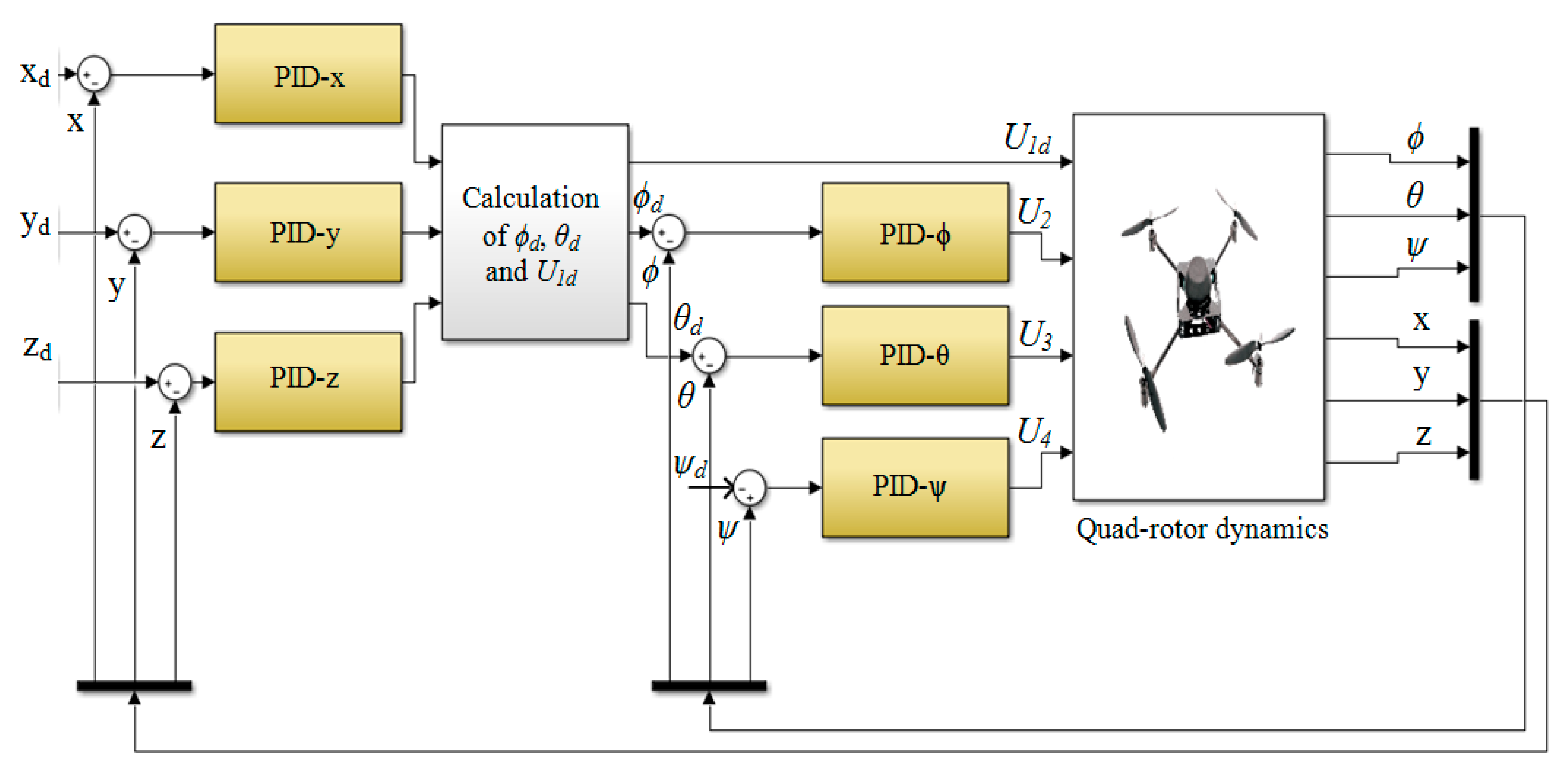
4. Quadrotor Control

4.1. Virtual Control

To manage the system dynamics, a simplified model is needed. By considering small rotations (cos x = 1 and sin x = x), the equations become linear and the PID controllers’ inputs can be clearly seen. Consequently, the control inputs for ϕ, θ, and ψ are U2, U3, and U4, respectively. To deal with the under-actuated part, ϕ, θ, and U1 are used to create three virtual control inputs so that every output will be controlled separately. Physically, these virtual controls mean that the translation motion along x, y, and z are controlled indirectly by the three common inputs (ϕ, θ, and U1). These virtual controls are given by Equation (19) and the desired trajectories of roll (ϕd), pitch (θd) and U1d are obtained by inverting Equation (19).
{ U x = ( c o s φ c o s ψ s i n θ + s i n φ s i n ψ ) U 1 U y = ( s i n ψ s i n θ c o s φ c o s ψ s i n φ ) U 1 U z = ( c o s φ c o s θ ) U 1
{ φ d = sin 1 ( U x   s i n ψ d U y   c o s ψ d U x 2 + U y 2 + U z 2 ) θ d = tan 1 ( U x   c o s ψ d + U y   s i n ψ d c o s φ d ) U 1 d = U x 2 + U y 2 + U z 2

4.2. Control Law Design

For an appropriate control of the UAV quadrotor system described by Equations (1)–(6), PID controllers are used. These controllers are simple to design and robust. The complete control scheme for the quadrotor is represented in Figure 2. It can be clearly seen from this figure that three PID controllers are used for positions (x, y, z) and three PIDs for attitudes (ϕ, θ, ψ). The inputs are divided to two parts, the desired and the sensor signals. Desired signals for positions and yaw angle (xd, yd, zd, ψd) are fixed by the pilot or the autopilot program. Sensor signals for desired roll and pitch angles (ϕd, θd, and U1d) are computed from the three virtual inputs Ux, Uy, and Uz.
The transfer functions Cs(p) of PID controllers are given in Equation (21), where s = {ϕ, θ, ψ, x, y, z}. Their gains (Kps, Kis, Kds) should be optimally tuned for the quadrotor in order to ensure stable, fast, precise, and robust responses. For this objective, PSO, CS, PSO-CS, and RM methods are applied to realize an optimal setting of these parameters.
C s ( p ) = K p s + K i s p + K d s p

4.3. Quadrotor Intelligent Control Using PSO, CS, and PSO-CS

To control the nonlinear and fully coupled quadrotor defined by Equations (1)–(6), it is suitable to use a method directly applicable to nonlinear systems as PSO, CS, and the cooperative PSO-CS. Instead of linear PID controllers, the intelligent and adaptive controllers can look for optimal PIDs parameters for the six quadrotors’ outputs [ϕ, θ, ψ, x, y, z].
The initial populations (N = 200) of PSO, CS, and PSO-CS are randomly dispersed in a search space that is chosen sufficient to contain all possible solutions [0, 200] and its dimension D is set to 18. To define the exploration capacity of each particle in order to improve the convergence of the process and to not exceed the velocity limits, we tested numerous values of w, and the compromise between local and global exploration in PSO was achieved for w = 0.8. The confidence coefficients C1 and C2 define the exploration capacity. They determine the degree of influence of the past positions of the particle itself and those of the other particles of the swarm in order to regulate the velocities relative to the best local and global positions, thus making it possible to determine the movements relative to these best positions. C1R1 and C2R2 are represented by matrices with dimension of 200 × swarm size. We considered that C1R1 takes random values in [0, 0.8] to avoid the problem of fast convergence, when C2R2 takes random values in [0, 1.2] to give more importance to the global best solution Pg (the interval of C2R2 is large to that of C1R1). In CS, the parameters used in experiments are as follows: Abandon probability Pa = 0.25, and the Lévy flights settings, α = 0.1 and λ = 1.5. In PSO-CS, the same settings of PSO and CS are conserved: Pa = 0.25, and the Lévy flights settings, α = 0.1, λ = 1.5 and C2 with random values in [0, 1.2].
To evaluate the optimization performance of the quadrotor’s responses using the proposed approaches, the fitness function (profit) is defined in a similar way in order to minimize the differences between the desired and the controlled outputs responses of the quadrotor. This fitness function is defined in Equation (22) as the sum of the errors Ek that characterize the difference in behavior between the inputs and the outputs of the quadrotor based on the Integral Square Error (ISE), with l = 6 and k = {1, 2, 3, 4, 5, 6}.
F = k = 1 l 0 E k 2 ( t ) d t
I S E = 0 E k 2 ( t ) d t
The performances found with ISE are compared to those established using three other performance indices: Integral Absolute Error (IAE), Integral Time Absolute Error (ITAE), and Integral Time Square Error (ITSE).
I A E = 0 | E k ( t ) | d t
I T A E = 0 t   | E k ( t ) | d t
I T S E = 0 t   E k 2 ( t ) d t
The maximum number of generations for the three programs (PSO, CS and PSO-CS) is fixed as the stop criterion and set to 20.

4.4. Quadrotor Classical Control Using RM

To use the linear RM technique for quadrotor control, the complete nonlinear Equations (1)–(6) should be simplified. The most used technique to simplify these nonlinear equations is to consider weak angles variations (reduced gyroscopic effects) and retain the linear portion, the Equations (1)–(6) become:
{ I x φ ¨ = l U 2 I y θ ¨ = l U 3 I z ψ ¨ = U 4 x ¨ = cos φ cos ψ sin θ + sin φ sin ψ m U 1 K f t x m x y ¨ = sin ψ sin θ cos φ cos ψ sin φ m U 1 K f t y m y z ¨ = g + cos φ cos θ m U 1 K f t z m z
The inputs U2, U3, U4, Ux, Uy, and Uz affect respectively angles of roll, pitch, and yaw, and positions x, y, and z, the reason for their usage as the PID controllers’ inputs. By applying the Laplace transform, we obtain the following transfer functions for angles (ϕ, θ, ψ) and positions (x, y, z).
{ G φ ( p ) = φ ( p ) U 2 ( p ) = l I x p 2 G θ ( p ) = θ ( p ) U 3 ( p ) = l I y p 2 G ψ ( p ) = ψ ( p ) U 4 ( p ) = 1 I z p 2 G x ( p ) = x ( p ) U x ( p ) = K x p ( τ x p + 1 ) G y ( p ) = y ( p ) U y ( p ) = K y p ( τ y p + 1 ) G z ( p ) = z ( p ) U z ( p ) = K z p ( τ z p + 1 )
where Kj = 1/Kftj, τj = m/Kftj and j = {x, y, z}.
For quadrotor’s attitudes and positions control, the behavior of the linear equations defined in (28) is approached to a desired reference one of a first order system. The desired behaviors for angles and positions correspond to the characteristic polynomials Rs(p), where s = {ϕ, θ, ψ, x, y, z} and α, α1, α2 are taken equal to 30, 2 and 30, respectively.
R s ( p ) = ( p + 1 τ ) ( p + α 1 τ ) ( p + α 2 τ )
For all cases, we calculate the closed loop transfer functions Hs(p) of the six systems including the PID controllers, for which we desire search their parameters. The computed denominators DHs(p) are given in Equation (30).
{ D H φ ( p ) = p 3 + l K d φ I x p 2 + l K p φ I x p + l K i φ I x D H θ ( p ) = p 3 + l K d θ I x p 2 + l K p θ I x p + l K i θ I x D H ψ ( p ) = p 3 + l K d ψ I x p 2 + l K p ψ I x p + l K i ψ I x D H x ( p ) = p 3 + K d x + K f t x m p 2 + K p x m p + K i x m D H y ( p ) = p 3 + K d y + K f t y m p 2 + K p y m p + K i y m D H z ( p ) = p 3 + K d z + K f t z m p 2 + K p z m p + K i z m

5. Results and Discussions

Simulations of the proposed intelligent and classical PID controllers are carried out on the quadrotor’s attitudes (ϕ, θ, ψ) and positions (x, y, z). These PIDs are tested firstly in the case of hovering to a determined position coordinates in order study the performances of the proposed intelligent PSO, CS and PSO-CS and the classical RM controllers. Then, for two different desired trajectories, the controllers’ gains are optimized through the intelligent proposed approaches. The main objective is to confirm the ability of these intelligent nature inspired methods to control the quadrotor and to efficiently realize different imposed trajectories even under the presence of disturbances. Table 1 gives the parameters of the quadrotor and Table 2 presents the suggested trajectories’ dynamics and their conditions.

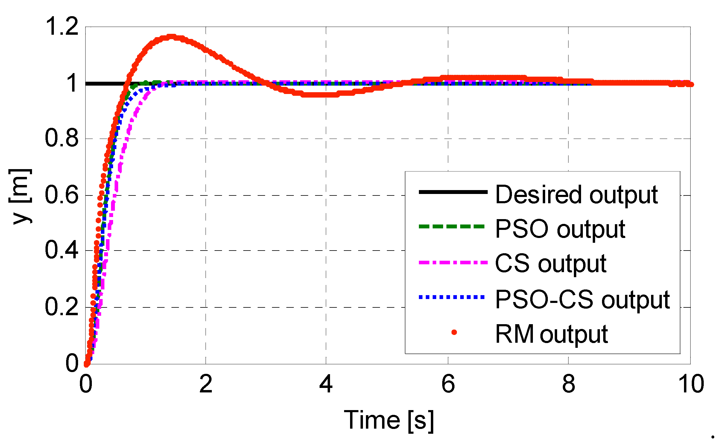
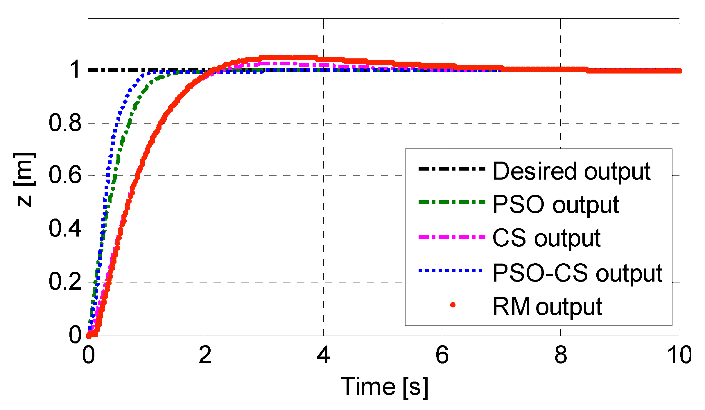
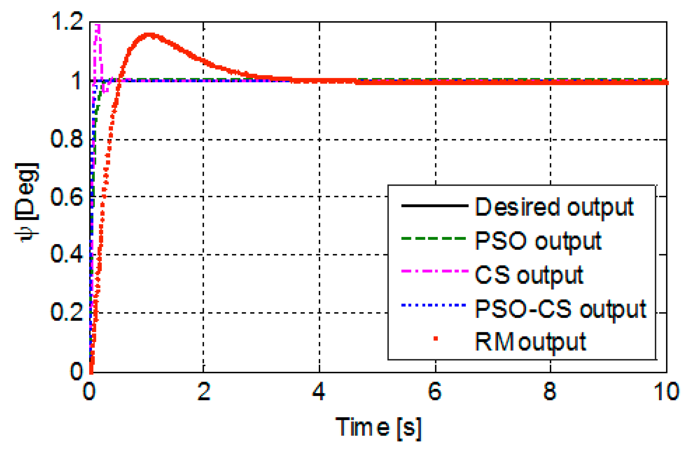
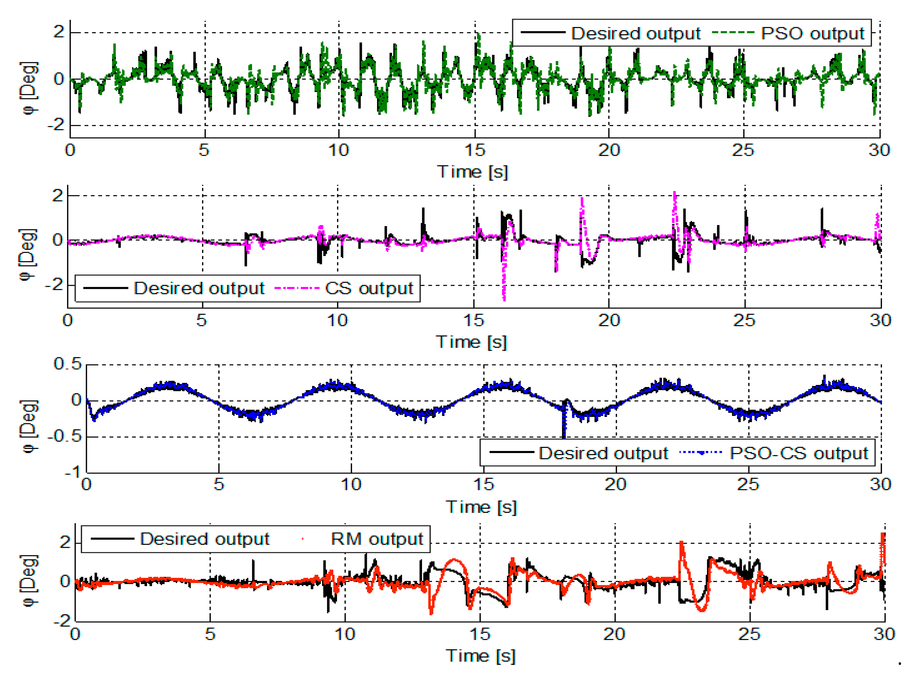
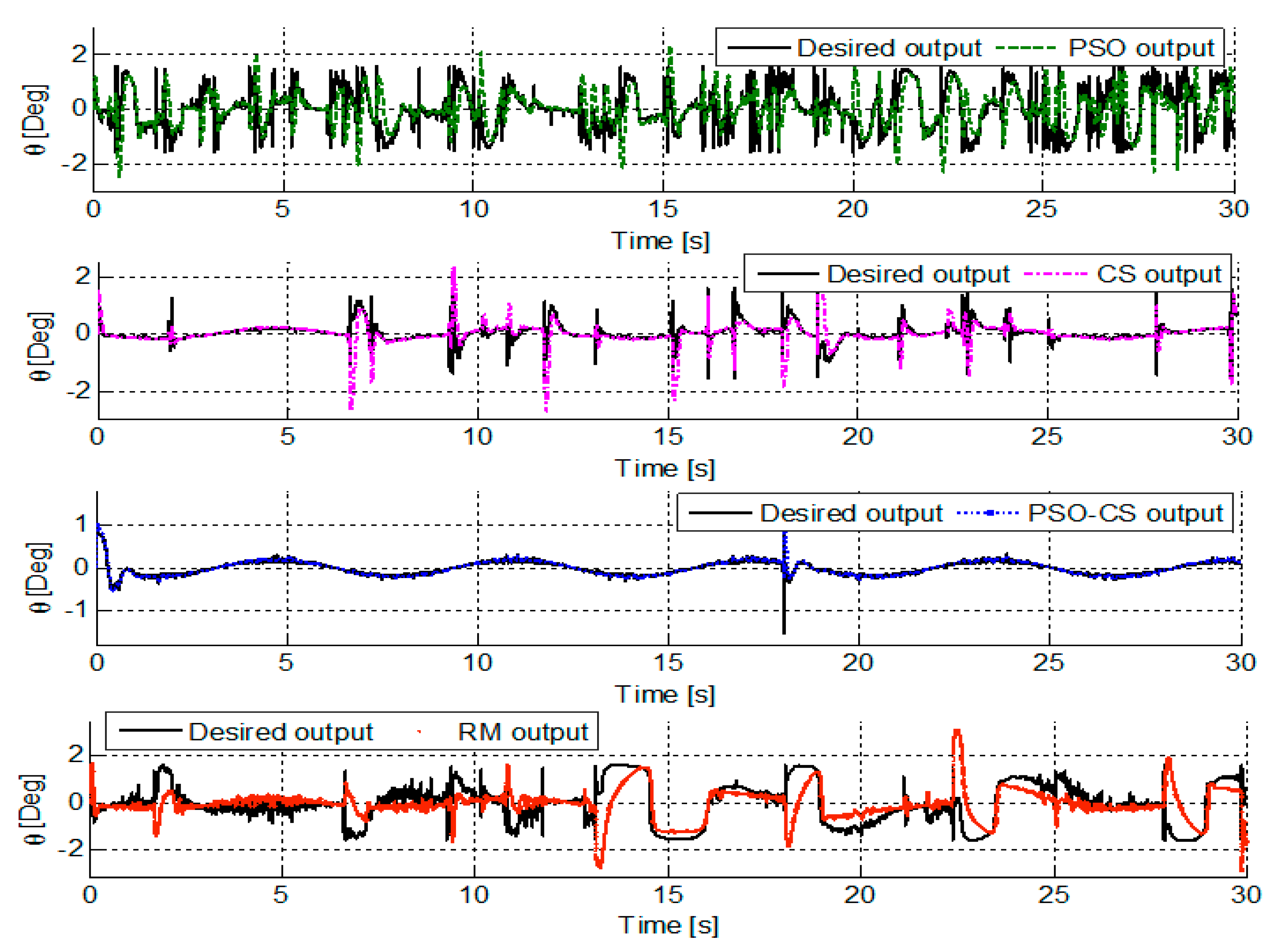
5.1. Comparisons of Intelligent and Classical Control Performances

To get the quadrotor to hover at a determined position coordinates, desired signals for positions [xd, yd, zd] are considered step signals of 1 m and desired yaw angle (ψd) is fixed to 1 degree. Table 3 summarizes the PID controllers gains computed online using PSO, CS, and PSO-CS, and offline with the conventional RM for the quadrotor’s outputs (ϕ, θ, ψ, x, y, z). Figure 3, Figure 4, Figure 5 and Figure 6 show the step responses for the corresponding outputs [x, y, z, ψ] obtained with these methods. Figure 7 and Figure 8 show the various obtained curves for the desired sensor signals as well as the controlled responses. Table 4 gives the obtained quadrotor’s responses performances: Settling time (Ts), maximum overshoot (Mp), and the errors previously mentioned (ISE, IAE, ITAE, and ITSE).
For control systems, the RM method often respects the fixed set of specifications and gives acceptable results [15]. However, this method is linear, and it cannot be applied directly to quadrotor control (the nonlinear quadrotor model). It can be observed from the obtained responses in Figure 3 and Figure 4 and the performances in Table 4 that the search for the parameters of PIDs by RM is not optimal: Responses with overshoots, settling times, and some error values exceed the amplitude of the desired signal. These unsatisfactory performances of the linear RM method in search of PID gains can be explained by the fact that the linear transfer functions defining the system (26) already have integrations.
CS results present a considerable overshoot in yaw angle and the errors values of ISE and IAE are around 50% of the desired altitude z, which proves that ISE value weight more significantly the quality of solutions and more adequate to evaluate the fitness function. However, the PSO approach is suitable and results in better performances. Comparisons of PSO results to those of Genetic Algorithms presented in Reference [16] show that PSO reduces the settling time Ts from 2.5 s to 0.172 s for yaw angle. For altitude z, the value of Ts is increased to 1.07 s instead of 0.4 s for GA. These results illustrate that PSO and GA techniques are highly competitive to explore the optimal solution in quadrotor control. In the same project of quadrotor control, the work presented in Reference [32] suggests three intelligent controllers, multilayer neural networks controller based on reference model (RMNN), Neural Networks with PD’s controller behavior (CPDNN), and Fuzzy Logic to adjust PID controllers’ gains (Fuzzy-PID). The proposed Fuzzy-PID and CPDNN achieves better performances compared to RMNN. Thus, comparing PSO results to those of Fuzzy-PID and CPDNN confirm that PSO is highly competitive to soft computing methods.
Considering the Figure 3, Figure 4, Figure 5, Figure 6, Figure 7 and Figure 8 and Table 4, the controllers tuned using PSO-CS have good performances for positions and attitudes. Thus, PSO-CS results are seen concurrent to those obtained using PSO, where responses lead to fast settling times with no overshoot and reduced errors. The desired sensor signal curves in Figure 7 and Figure 8 (desired roll and pitch angles (ϕd and θd)) depend on the outputs of the controllers PID-x, PID-y, and PID-z. It is observed from this figure that these intelligent approaches, and especially PSO and PSO-CS, allow to follow perfectly the sensor signals for roll and pitch (ϕd and θd), and give controlled responses close to the desired curves.
These programs are implemented using Matlab R2016a and performed on a computer with a processor Intel® Core™ i7-3770 CPU of 3.40 GHz and 8.0 GB of RAM. From the conducted experiments, we can get conclusions that for the same goal, the PSO algorithm spends less CPU time (10 min 45 s) than the PSO-CS algorithm (14 min 12 s) and the CS algorithm (12 min 15 s). During the calculation of the velocity update equation, PSO-CS consumes an additional CPU time as the algorithm combines the two matrices generating Lévy flights random walks of cuckoos and that generating the movement of particles toward the global best solution Pg. However, the PSO-CS and PSO algorithms get higher performances (reduced errors) than the CS algorithm and RM method. These results are achieved thanks to the good adjustment of PSO, CS and PSO-CS parameters: Position and velocity initializations, the appropriate choice of the fitness function, the good tuning of the weighting coefficients w, C1, and C2, the chosen probability Pa, and the Lévy flights settings for α and λ.

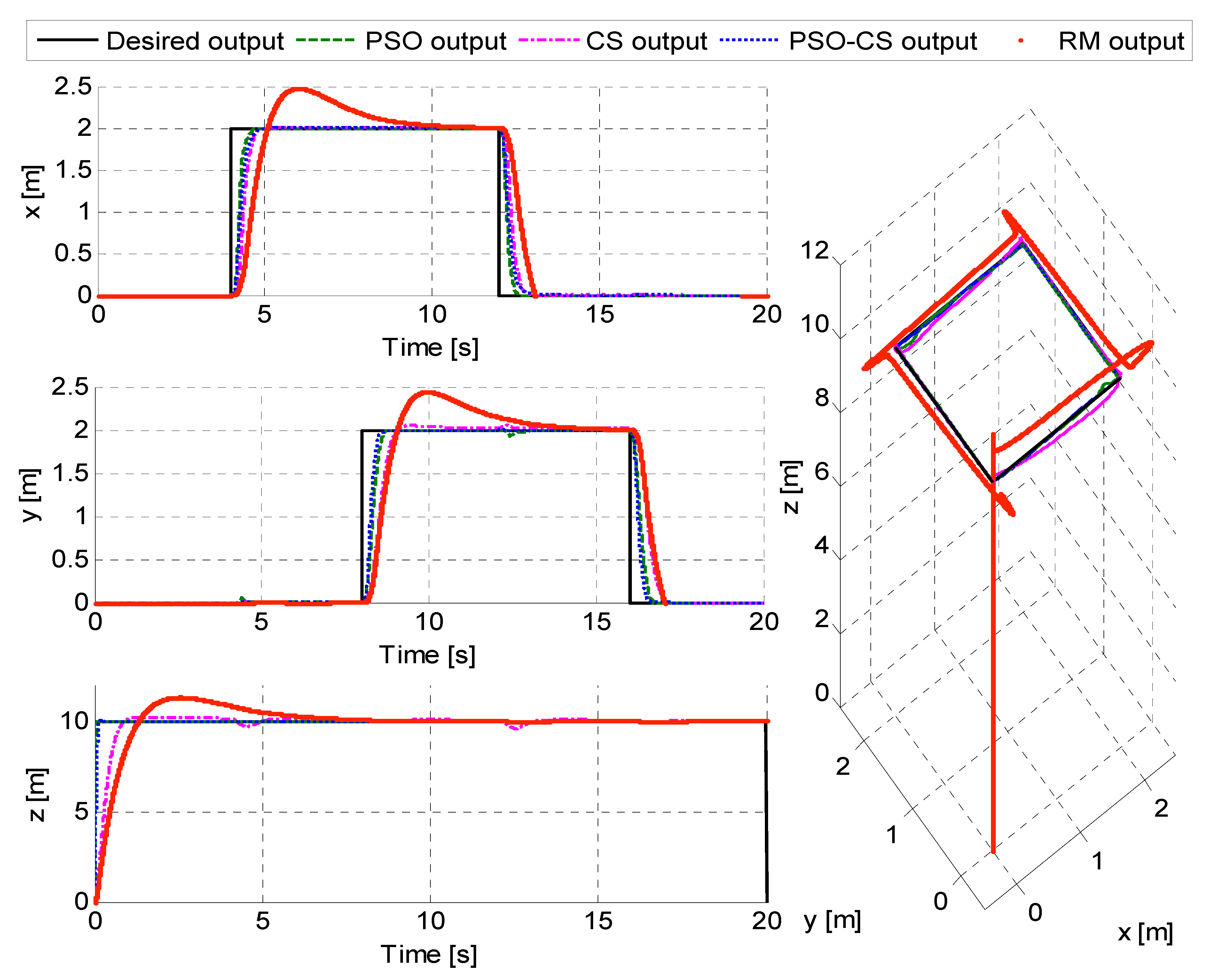
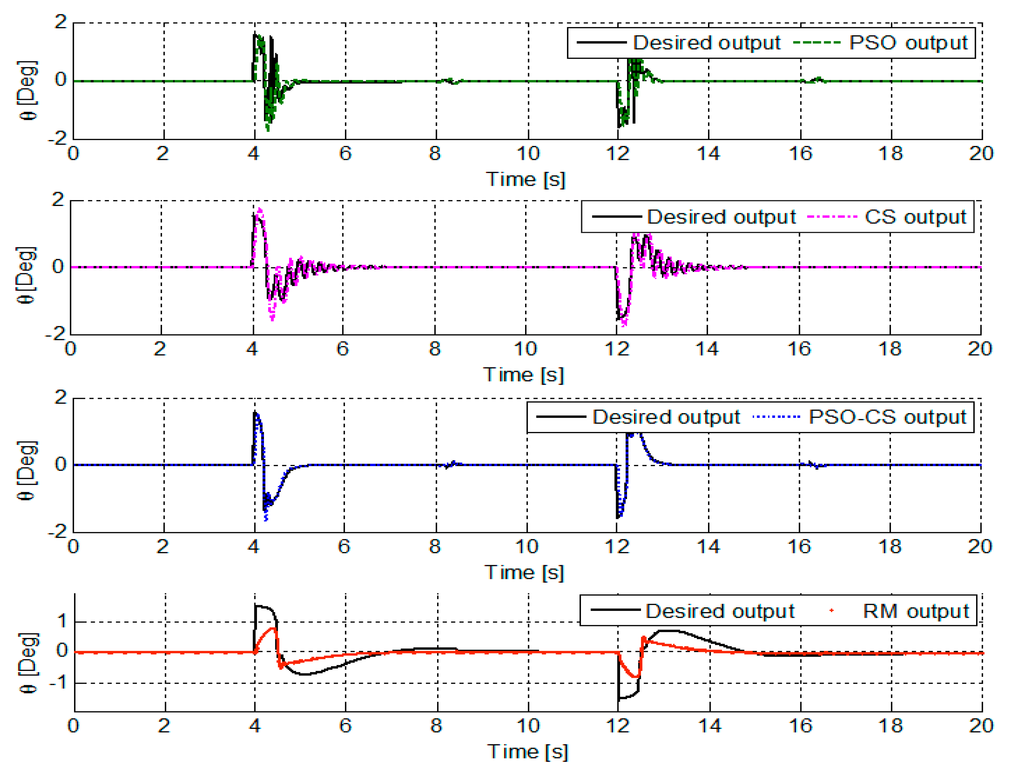
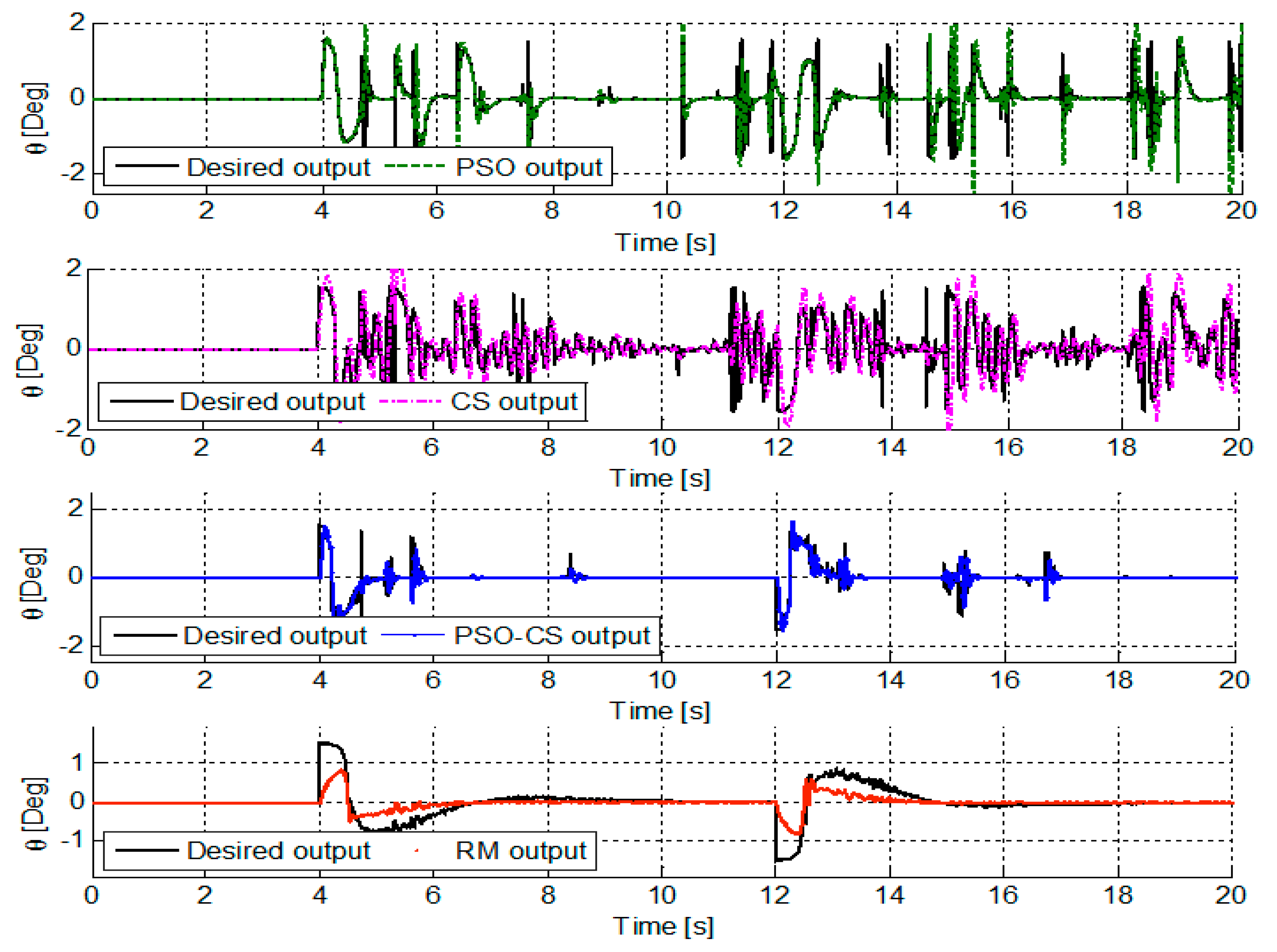
5.2. Rectangular Trajectory Tracking

This experimental simulation on the quadrotor engages to test the PIDs’ efficiency when the vehicle tracks a square trajectory without overturning. In this mode, inputs for desired positions (xd, yd, zd) are considered pulse signals and desired yaw attitude is set to 0°. Figure 9 shows the tracking of each position coordinate (x, y, z) and the tracking trajectories in 3D plan obtained using the proposed methods. Responses for desired and controlled roll (ϕ) and pitch (θ) attitudes are illustrated in Figure 6. Table 5 resumes the errors ISE used to compute fitness function.
It can be noticeably observed from Figure 9 and Table 5 that the adaptive autotuned controllers using PSO, CS, and PSO-CS have good performances (reduced errors) for positions (x, y, z) control. PSO-CS and PSO responses always lead to fast settling times with no overshoot for x position. RM presents overshoots for positions and CS shows few overshoots for y position and altitude z. The intelligent PSO and the cooperative PSO-CS drive the system toward perfect tracking of the prescribed square trajectory. Also, all these methods allowed maintaining the yaw angle in zero degrees: no overturning of the aircraft. Figure 10 and Figure 11 confirm that these intelligent approaches of PSO-CS nd PSO give controlled responses closed to the desired roll and pitch attitudes.
To test the robustness of these PID controllers, external disturbance was introduced. The most likely disturbance acting on the quadrotor is the wind disturbance along z axis. The external disturbance is modeled in this simulation by a random signal of variable amplitude inserted in the closed loop scheme of altitude z. It is noticed from Figure 12, Figure 13 and Figure 14 and the errors ISE presented in Table 6 that when random disturbance affects the quadrotor, PSO, CS, and PSO-CS controllers reject these undesirable effects and provide outputs responses close to the desired ones. Therefore, we can affirm that PSO, CS, and especially the cooperative PSO-CS, are able to tune optimally the six PID controllers and drive the quadrotor to the desired altitude z, positions x and y, and yaw angle.

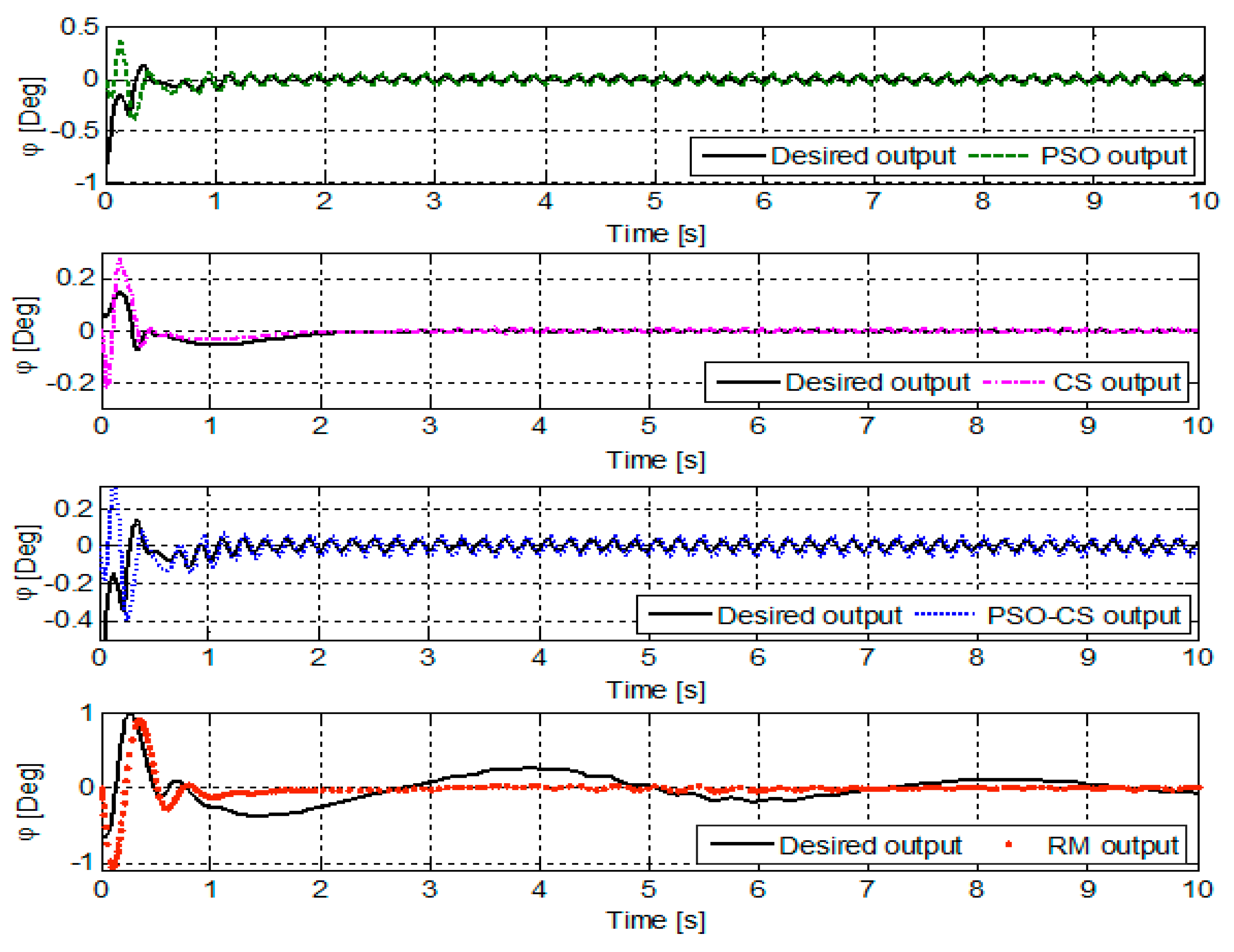
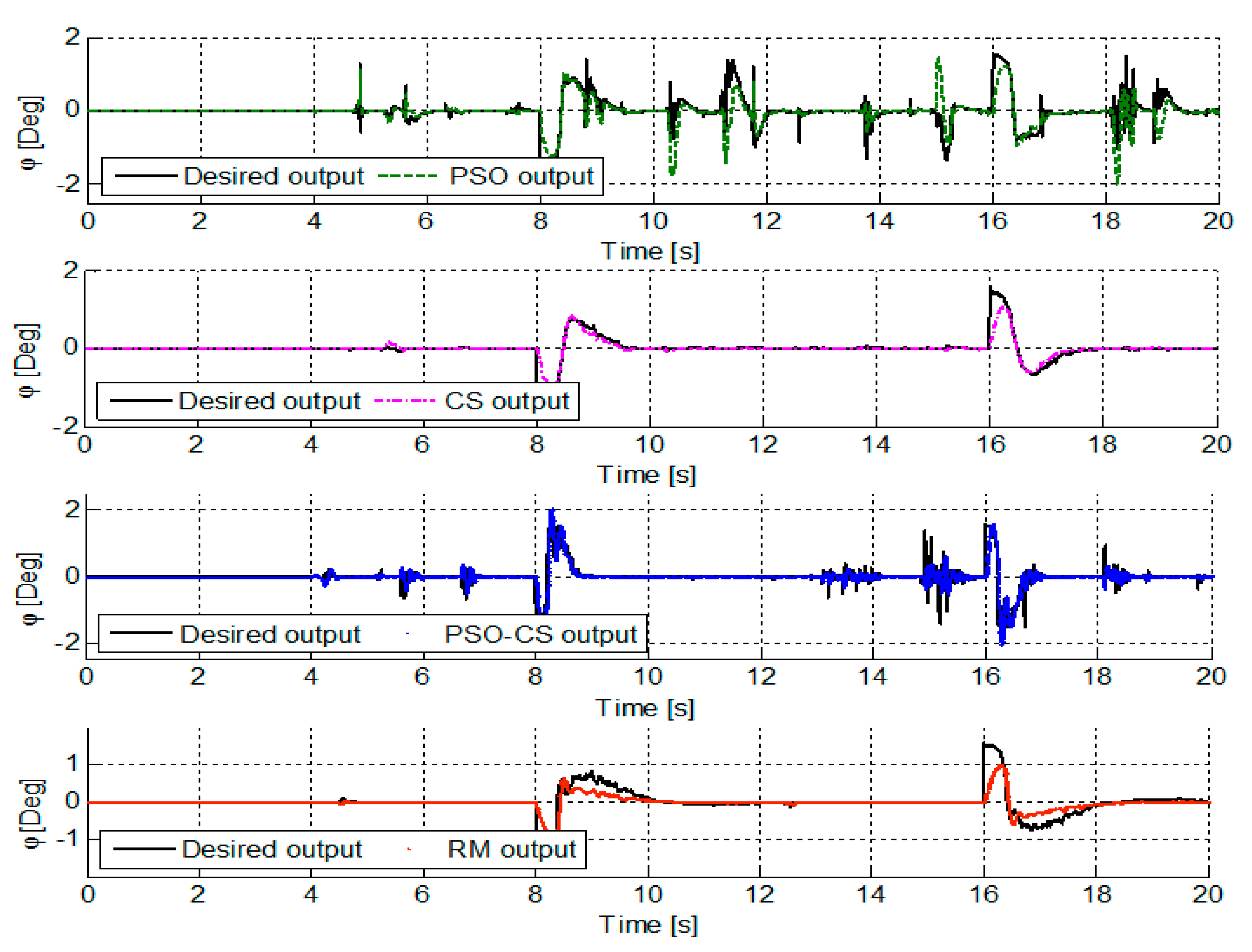
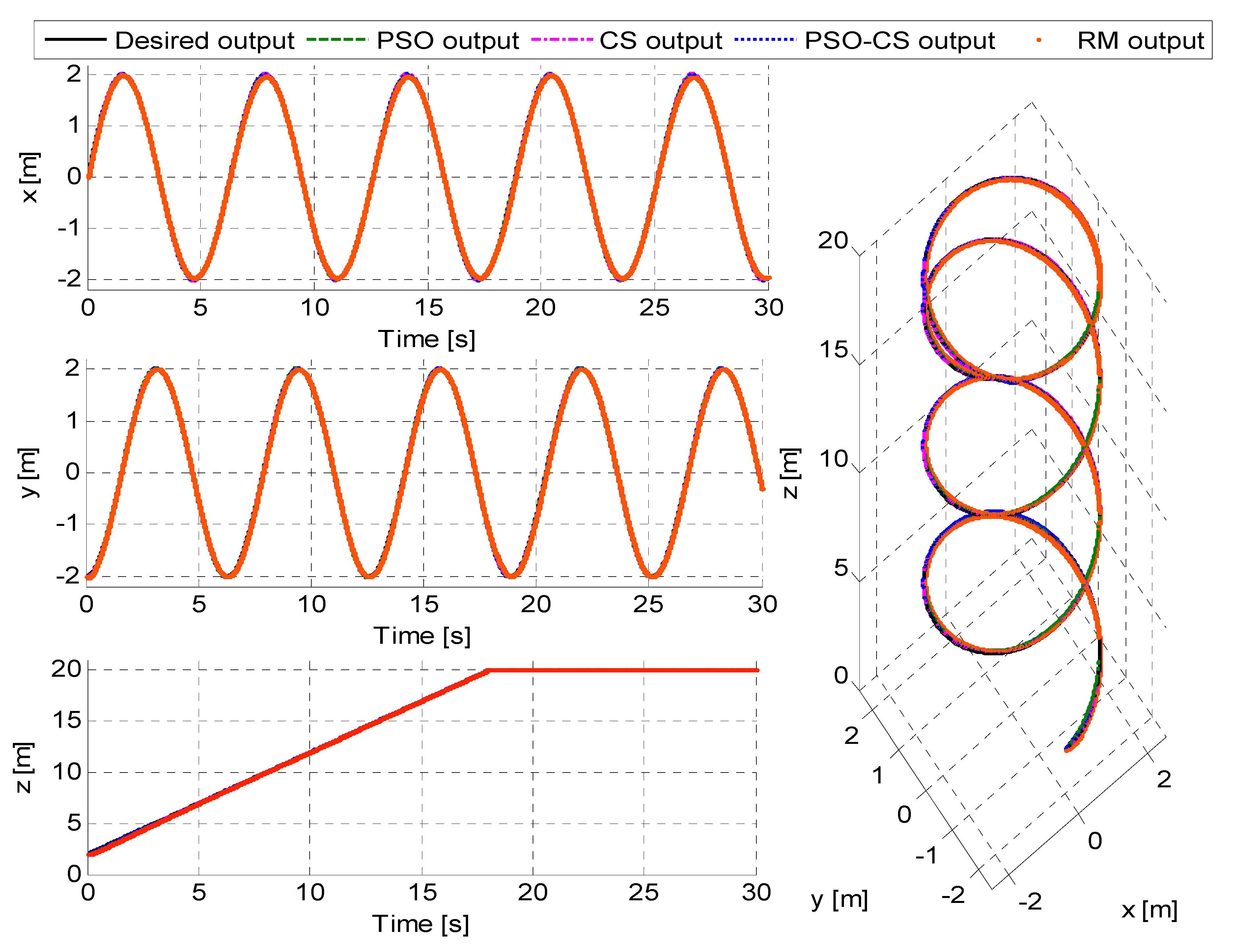
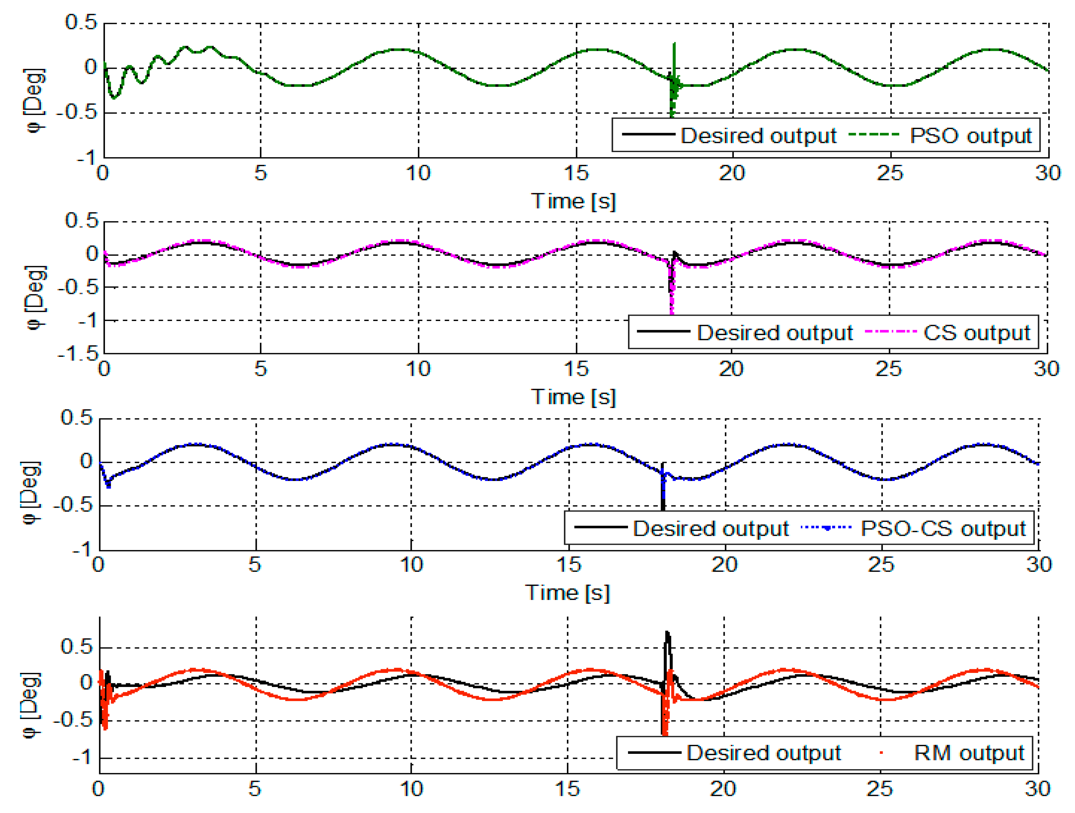
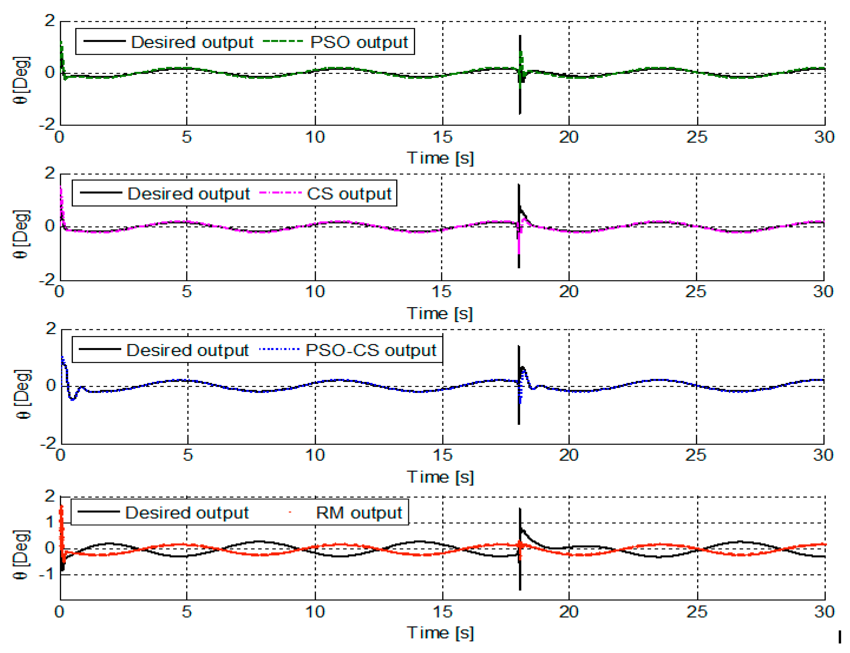
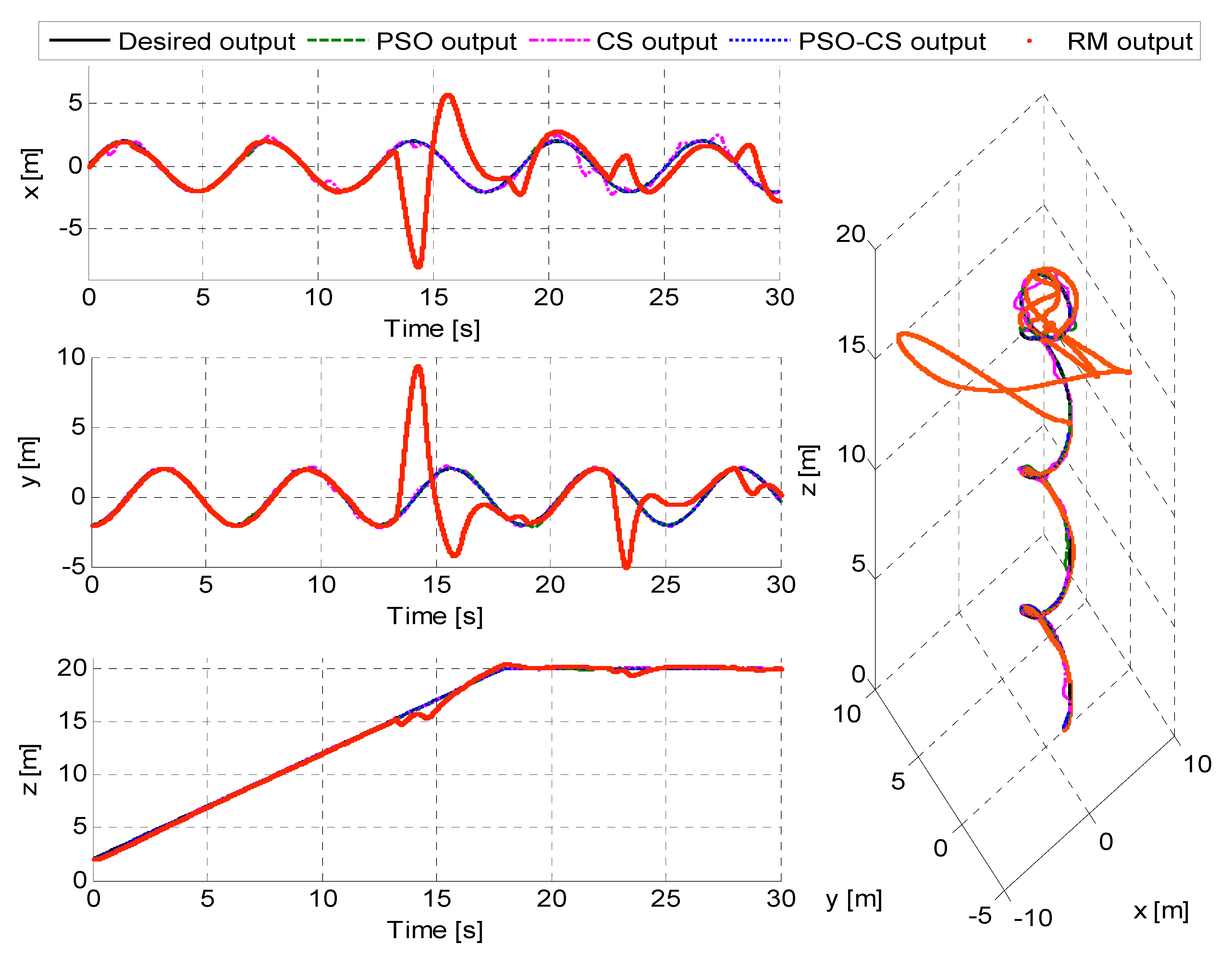
5.3. Helical Trajectory Tracking

Through the last simulation, we will investigate more the efficiency of the proposed intelligent control methods (PSO, CS, and PSO-CS) to search for optimal PID autotuned controllers for the quadrotor, when the desired trajectory is a helix. Simulation results of each position’s tracking (x, y, z), and the tracking in 3D plan are presented in Figure 15. The tracking of roll and pitch attitudes (ϕ and θ) are presented in Figure 16 and Figure 17. Table 7 summarizes the obtained ISE errors.
Figure 15 clearly shows the possibility of the quadrotor system to follow a linear movement in altitude z in the first mode from 0 to 18 s and to keep perfectly a stable attitude z of 20 m in the second mode from 18 to 30 s. For translation motion, the quadrotor makes a complete circle of 2 m of radius in 30 s, where we notice that the errors in x, y, and z axis are very small (from Table 7). The same figure illustrates in 3D plan that the quadrotor tracks the helix trajectory and ends by a circle form. Also, the quadrotor avoids with high precision the overturning and maintains exactly 0° in yaw attitude.
Figure 16 and Figure 17 and Table 7 illustrate that PSO, CS, and PSO-CS help to follow perfectly the sensor signals (ϕd and θd). These results prove the possibility of our system to follow the imposed combined trajectory form with precision, for all variables (positions (x and y), altitude z, and attitudes (ϕ, θ, and ψ).
These controllers are tested in order to evaluate their performances under the same disturbance (a random input of variable amplitude) inserted in the altitude z closed loop scheme of the quadrotor. It can be observed from Figure 18, Figure 19 and Figure 20 and Table 8 that PSO and PSO-CS controllers reject the disturbance effects and drive all variables to the desired ones. Therefore, we can affirm that despite the usage of a combined trajectory form and the presence of forcible disturbance, adaptive PSO-CS and PSO are proven as remarkably robust and efficient for quadrotor control.

6. Conclusions

In this paper, Particle Swarm Optimization (PSO), Cuckoo Search (CS), and the proposed cooperative PSO-CS were applied to control the quadrotor system. Results proved the efficiency of PSO approach and the cooperative PSO-CS to control optimally the quadrotor’s outputs (ϕ, θ, ψ, x, y, z) compared to CS and the classical Reference Model (RM) methods. Experimental simulations also confirm the effectiveness of the aircraft using the proposed intelligent PID controllers to track the imposed rectangular and helical trajectories. Indeed, the robustness and performances of the intelligent controllers are validated in presence of disturbance. The performances of PSO-CS showed not only the stability robustness against the external disturbance, but also the fast response and the excellent tracking capacity for the different trajectories. These achievements are the results of the good settings of PSO, CS, and PSO-CS parameters. The advantages of the proposed PSO-CS in seeking for the best solutions in control problem are the results of exploiting the local search capacity of CS and benefiting from the global intelligence offered by PSO.
Concerning the limitations of our PSO-CS, one more parameter is added to CS program, which is the acceleration constant C2. A wrong setting of this parameter can cause premature convergence. C2 makes the cuckoos move toward the global best solution and must ensure a compromise between local and global exploration of the search space. On the other hand, the PSO-CS program consumes additional CPU time to calculate the velocity update equation over generations in order to perform the search.

Author Contributions

Data curation, N.E.; Investigation, N.E. and M.M.; Methodology, N.E. and M.M.; Ressources, N.E.; built the Simulation program and was also responsible for writing the paper. M.M.; Supervision, M.M., A.E.K., and H.A.; Validation M.M; Writing–original draft, N.E; Writing–review and editing, N.E. and M.M.

Funding

This research received no external funding.

Conflicts of Interest

The authors declare no conflict of interest.

Abbreviations

ACSAdaptive Cuckoo Search
CSCuckoo Search
ISEIntegral Square Error
IAEIntegral Absolute Error
ITSEIntegral Time Square Error
ITAEIntegral Time Absolute Error
PIProportional and Integral
PIDProportional, Integral and Derivative
PDProportional and Derivative
PSOParticle Swarm Optimization
PSO-CSParticle Swarm Optimization-Cuckoo Search
RMReference Model
UAVUnmanned Aerial Vehicles

References

  1. Bouabdallah, S.; Murrieri, P.; Siegwart, R. Design and control of an indoor micro quadrotor. In Proceedings of the IEEE International Conference in Robotics and Automation, New Orleans, LA, USA, 26 April–1 May 2004; pp. 4393–4398. [Google Scholar]
  2. Bouabdallah, S. Design and Control of Quadrotors with Application to Autonomous Flying. Ph.D. Dissertation, Ecole Polytechnique Federale de Lausanne, Lausanne, Suisse, 2007. [Google Scholar]
  3. Bouabdallah, S.; Noth, A.; Siegwart, R. PID vs. LQ control techniques applied to an indoor micro quadrotor. In Proceedings of the IEEE International Conference in Intelligent Robots and Systems, Sendai, Japan, 28 September–2 October 2004; pp. 2451–2456. [Google Scholar]
  4. Naidoo, Y.; Stopforth, R.; Bright, G. Quadrotor Unmanned Aerial Vehicle Helicopter Modelling & Control. Int. J. Adv. Robot. Syst. 2011, 8, 139–149. [Google Scholar]
  5. Besnard, L.; Shtessel, Y.B.; Landrum, B. Quadrotor vehicle control via sliding mode controller driven by sliding mode disturbance observer. J. Frankl. Inst. 2012, 349, 658–684. [Google Scholar] [CrossRef]
  6. Honglei, A.; Jie, L.; Jian, W.; Jianwen, W.; Hongxu, M. Backstepping-based inverse optimal attitude control of quadrotor. Int. J. Adv. Robot. Syst. 2013, 10, 9. [Google Scholar] [CrossRef]
  7. Amin, R.; Aijun, L.; Shamshirband, S. A review of quadrotor UAV: Control methodologies and performance evaluation. Int. J. Autom. Control 2016, 10, 87–103. [Google Scholar] [CrossRef]
  8. Astrom, K.J. PID Controllers: Theory, Design and Tuning; Instrument Society of America: Research Triangle Park, NC, USA, 1995. [Google Scholar]
  9. Salih, A.L.; Moghavvemi, M.; Mohamed, H.; Gaeid, K.S. Flight PID controller design for a UAV quadrotor. Sci. Res. Essays 2010, 5, 3660–3667. [Google Scholar]
  10. Junior, J.C.V.; De Paula, J.C.; Leandro, G.V.; Bonfim, M.C. Stability control of a quadrotor using a PID controller. J. Appl. Instrum. Control 2013, 1, 15–20. [Google Scholar]
  11. Astrom, K.J.; Hagglund, T. Revisiting the Ziegler-Nichols step response method for PID control. J. Process Control 2004, 14, 635–650. [Google Scholar] [CrossRef]
  12. Graham, D.; Lathrop, R.C. The synthesis of optimum transient response: Criteria and standard forms. Trans. AIEE 1953, 72, 273–288. [Google Scholar] [CrossRef]
  13. Naslin, P. Essentials of Optimal Control; Iliffe & Sons Ltd.: London, UK, 1968. [Google Scholar]
  14. Mjahed, M. Control of Systems; Royal School of Aeronautics: Marrakech, Morocco, 2016. [Google Scholar]
  15. El gmili, N.; Mjahed, M.; EL Kari, A.; Ayad, H. An Improved Particle Swarm Optimization (IPSO) Approach for Identification and Control of Stable and Unstable Systems. Int. Rev. Autom. Control 2017, 10, 229–239. [Google Scholar] [CrossRef]
  16. Siti, I.; Mjahed, M.; El Kari, A.; Ayad, H. New Designing Approaches for Quadcopter PID Controllers Using Reference Model and Genetic Algorithm Techniques. Int. Rev. Autom. Control 2017, 10, 240–248. [Google Scholar] [CrossRef]
  17. Mjahed, M. Optimization of classification tasks by using genetic algorithms. In Proceedings of the 7th IEEE International Conference on Informatics and Systems, Cairo, Egypt, 28–30 March 2010; pp. 1–4. [Google Scholar]
  18. Kennedy, J.; Eberhart, R.C. Particle swarm optimization. In Proceedings of the IEEE International Conference on Neural Networks, Perth, Australia, 27 November–1 December 1995; pp. 1942–1948. [Google Scholar]
  19. Mohan, B.C.; Baskaran, R. A survey: Ant colony optimization based recent research and implementation on several engineering domain. Expert Syst. Appl. 2012, 39, 4618–4627. [Google Scholar]
  20. Karaboga, D.; Gorkemli, B.; Ozturk, C.; Karaboga, N. A comprehensive survey: Artificial bee colony (ABC) algorithm and applications. Artif. Intell. Rev. 2014, 42, 21–57. [Google Scholar]
  21. Joshi, A.S.; Kulkarni, O.; Kakandikar, G.M.; Nandedkar, V.M. Cuckoo Search Optimization—A Review. Mater. Today Proc. 2017, 4, 7262–7269. [Google Scholar] [CrossRef]
  22. Kamoona, A.M.; Patra, J.C.; Stojcevski, A. An Enhanced Cuckoo Search Algorithm for Solving Optimization Problems. In Proceedings of the IEEE Congress on Evolutionary Computation (CEC), Rio de Janeiro, Brazil, 8–13 July 2018; pp. 1–6. [Google Scholar]
  23. Chaine, S.; Tripathy, M. Design of an optimal SMES for automatic generation control of two-area thermal power system using cuckoo search algorithm. J. Electr. Syst. Inf. Technol. 2015, 2, 1–13. [Google Scholar] [CrossRef]
  24. Zamani, A.A.; Tavakoli, S.; Etedali, S. Fractional order PID control design for semi-active control of smart base-isolated structures: A multi-objective cuckoo search approach. ISA Trans. 2017, 67, 222–232. [Google Scholar] [CrossRef] [PubMed]
  25. Sona, D.R. PSO algorithm in quadcopter cluster for unified trajectory planning using wireless ad hoc network. In Proceedings of the International Conference on Soft Computing Systems; Springer: New Delhi, India, 2015; pp. 819–826. [Google Scholar]
  26. Noordin, A.; Basri, M.A.M.; Mohamed, Z.; Abidin, A.F.Z. Modelling and PSO Fine-tuned PID Control of Quadrotor UAV. Int. J. Adv. Sci. Eng. Inf. Technol. 2017, 7, 1367–1373. [Google Scholar] [CrossRef]
  27. Abbas, N.H.; Sami, A.R. Tuning of PID Controllers for Quadcopter System using Hybrid Memory based Gravitational Search Algorithm–Particle Swarm Optimization. Int. J. Comput. Appl. 2018, 172, 80–99. [Google Scholar]
  28. Naik, M.; Nath, M.R.; Wunnava, A.; Sahany, S.; Panda, R. A new adaptive Cuckoo search algorithm. In Proceedings of the 2nd International Conference on Recent Trends in Information Systems (ReTIS), Kolkata, India, 9–11 July 2015; pp. 1–5. [Google Scholar]
  29. Marini, F.; Walczak, B. Particle swarm optimization (PSO). A tutorial. Chemom. Intell. Lab. Syst. 2015, 149, 153–165. [Google Scholar] [CrossRef]
  30. Clerc, M.; Kennedy, J. The particle swarm-explosion, stability, and convergence in a multidimensional complex space. IEEE Trans. Evol. Comput. 2002, 6, 58–73. [Google Scholar] [CrossRef]
  31. Dréo, J.; Siarry, P. Métaheuristiques pour L’optimisation Difficile; Eyrolles: Paris, France, 2003. [Google Scholar]
  32. El Hamidi, K.; Mjahed, M.; El Kari, A.; Ayad, H. Neural and Fuzzy Based Nonlinear Flight Control for an Unmanned Quadcopter. Int. Rev. Autom. Control 2018, 11, 98–106. [Google Scholar] [CrossRef]
Figure 1. Quadrotor’s configuration.
Applsci 09 01719 g001
Figure 2. Complete control scheme for quadrotor.
Applsci 09 01719 g002
Figure 3. Quadrotor’s position x using Particle Swarm Optimization (PSO), Cuckoo Search (CS), Particle Swarm Optimization-Cuckoo Search (PSO-CS), and Reference Model (RM).
Applsci 09 01719 g003
Figure 4. Quadrotor’s position y using Particle Swarm Optimization (PSO), Cuckoo Search (CS), Particle Swarm Optimization-Cuckoo Search (PSO-CS), and Reference Model (RM).
Applsci 09 01719 g004
Figure 5. Quadrotor’s altitude z using Particle Swarm Optimization (PSO), Cuckoo Search (CS), Particle Swarm Optimization-Cuckoo Search (PSO-CS), and Reference Model (RM).
Applsci 09 01719 g005
Figure 6. Quadrotor’s yaw attitude (ψ) using Particle Swarm Optimization (PSO), Cuckoo Search (CS), Particle Swarm Optimization-Cuckoo Search (PSO-CS), and Reference Model (RM).
Applsci 09 01719 g006
Figure 7. Quadrotor’s roll attitude (ϕ) using Particle Swarm Optimization (PSO), Cuckoo Search (CS), Particle Swarm Optimization-Cuckoo Search (PSO-CS), and Reference Model (RM).
Applsci 09 01719 g007
Figure 8. Quadrotor’s pitch attitude (θ) using Particle Swarm Optimization (PSO), Cuckoo Search (CS), Particle Swarm Optimization-Cuckoo Search (PSO-CS), and Reference Model (RM).
Applsci 09 01719 g008
Figure 9. Quadrotor’s positions (x, y, z) using Particle Swarm Optimization (PSO), Cuckoo Search (CS), Particle Swarm Optimization-Cuckoo Search (PSO-CS), and Reference Model (RM) (rectangular trajectory).
Applsci 09 01719 g009
Figure 10. Quadrotor’s roll attitude (ϕ) using Particle Swarm Optimization (PSO), Cuckoo Search (CS), Particle Swarm Optimization-Cuckoo Search (PSO-CS), and Reference Model (RM) (rectangular trajectory).
Applsci 09 01719 g010
Figure 11. Quadrotor’s pitch attitude (θ) using Particle Swarm Optimization (PSO), Cuckoo Search (CS), Particle Swarm Optimization-Cuckoo Search (PSO-CS), and Reference Model (RM) (rectangular trajectory).
Applsci 09 01719 g011
Figure 12. Quadrotor’s positions (x, y, z) using Particle Swarm Optimization (PSO), Cuckoo Search (CS), Particle Swarm Optimization-Cuckoo Search (PSO-CS), and Reference Model (RM) with disturbance (rectangular trajectory).
Applsci 09 01719 g012
Figure 13. Quadrotor’s roll attitude (ϕ) using Particle Swarm Optimization (PSO), Cuckoo Search (CS), Particle Swarm Optimization-Cuckoo Search (PSO-CS), and Reference Model (RM) with disturbance (rectangular trajectory).
Applsci 09 01719 g013
Figure 14. Quadrotor’s pitch attitude (θ) using Particle Swarm Optimization (PSO), Cuckoo Search (CS), Particle Swarm Optimization-Cuckoo Search (PSO-CS), and Reference Model (RM) with disturbance (rectangular trajectory).
Applsci 09 01719 g014
Figure 15. Quadrotor’s positions (x, y, z) using Particle Swarm Optimization (PSO), Cuckoo Search (CS), Particle Swarm Optimization-Cuckoo Search (PSO-CS), and Reference Model (RM) (helical trajectory).
Applsci 09 01719 g015
Figure 16. Quadrotor’s roll attitude (ϕ) using Particle Swarm Optimization (PSO), Cuckoo Search (CS), Particle Swarm Optimization-Cuckoo Search (PSO-CS), and Reference Model (RM) (helical trajectory).
Applsci 09 01719 g016
Figure 17. Quadrotor’s pitch attitude (θ) using Particle Swarm Optimization (PSO), Cuckoo Search (CS), Particle Swarm Optimization-Cuckoo Search (PSO-CS), and Reference Model (RM) (helical trajectory).
Applsci 09 01719 g017
Figure 18. Quadrotor’s positions (x, y, z) Particle Swarm Optimization (PSO), Cuckoo Search (CS), Particle Swarm Optimization-Cuckoo Search (PSO-CS), and Reference Model (RM) with disturbance (helical trajectory).
Applsci 09 01719 g018
Figure 19. Quadrotor’s roll attitude (ϕ) using Particle Swarm Optimization (PSO), Cuckoo Search (CS), Particle Swarm Optimization-Cuckoo Search (PSO-CS), and Reference Model (RM) with disturbance (helical trajectory).
Applsci 09 01719 g019
Figure 20. Quadrotor’s pitch attitude (θ) using Particle Swarm Optimization (PSO), Cuckoo Search (CS), Particle Swarm Optimization-Cuckoo Search (PSO-CS), and Reference Model (RM) with disturbance (helical trajectory).
Applsci 09 01719 g020
Table 1. Quadrotor’s parameters.
Parameter (unit)Value
m (Kg)0.65
g (m/s2)9.806
l (m)0.4
b (N/rad/s)2.9842 × 10−5
d (N.m/rad/s)7.5 × 10−7
Ix, Iy (Kg.m2)7.5 × 10⁻³
Iz (Kg.m2)1.3 × 10⁻³
Jr (Kg.m2)2.8385 × 10⁻⁵
Kfax, Kfay (N/rad/s)5.567 × 10−4
Kfaz (N/rad/s)6.354 × 10−4
Kftx, Kfty(N/rad/s)5.567 × 10−4
Kftz (N/rad/s)3.354 ×10−4
Table 2. Trajectories’ conditions and dynamics.
Initial ConditionsTrajectory DescriptionAttitude’s Saturation
Rectangular
Trajectory
[ϕ, θ, ψ, x, y, z] =
[0, 0, 0, 0, 0, 10]
x d ( t ) = 2 [ u ( t 4 ) u ( t 12 ) ] y d ( t ) = 2 [ u ( t 8 ) u ( t 16 ) ] z d ( t ) = 10 u ( t 20 ) ψ d ( t ) = 0 −90° < ϕ, θ < 90
Helical Trajectory[ϕ, θ, ψ, x, y, z] =
[0, 0, 0, 0, 0, 2]
x d ( t ) = 2 sin ( 2 π t ) y d ( t ) = 2 sin ( 2 π t π / 2 ) z d ( t ) = t u ( t ) ( t 18 ) u ( t 18 ) ψ d ( t ) = 0
Table 3. Optimal Proportional, Integral and Derivative (PID) parameters obtained with Particle Swarm Optimization (PSO), Cuckoo Search (CS), Particle Swarm Optimization-Cuckoo Search (PSO-CS), and Reference Model (RM) for the quadrotor.
Quadrotor’s
Output
Optimal PID Gains
PSOCS
KpKiKdKpKiKd
x42.8290.16712.36627.3450.86514.023
y62.8810.22616.06536.7140.50514.056
z34.54514.5089.49814.7568.6478.077
ϕ14.7401.7490.97517.9480.1781.055
θ13.8720.8090.55519.4300.8671.806
ψ15.2990.7020.9947.9670.1980.278
PSO-CSRM
KpKiKdKpKiKd
x69.822−0.01116.97459.15029.25030.550
y45.8800.00815.06739.65019.50020.800
z31.85917.7246.71526.06610.39416.865
ϕ206.6173.9411.4932.7392.6080.783
θ121.842−1.6482.2173.2931.6301.695
ψ38.4690.4691.4661.0921.0400.31
Table 4. Performances obtained with Particle Swarm Optimization (PSO), Cuckoo Search (CS), Particle Swarm Optimization-Cuckoo Search (PSO-CS), and Reference Model (RM) for the quadrotor.
OutputPerformancesMethod
PSOCSPSO-CSRM
xTs (s)0.7301.3840.5223.779
Mp (%)0.4121.7690.44622.869
ISE0.2270.3460.16500.365
IAE0.3240.4920.2340.714
ITSE0.0340.0830.0180.176
ITAE0.0880.2620.0380.847
yTs (s)0.6751.0180.7823.517
Mp (%)0.4970.8980.01030.741
ISE0.2370.2960.2260.441
IAE0.3220.4100.3190.802
ITSE0.0360.0580.0340.245
ITAE0.0830.1520.0760.954
zTs (s)1.0701.8210.8131.855
Mp (%)0.1072.4630.0023.467
ISE0.2430.4060.2080.342
IAE0.3970.5870.3080.617
ITSE0.0500.1290.0310.122
ITAE0.1340.3120.0810.521
ϕISE0.0280.0060.0050.093
IAE0.1970.0530.0320.431
ITSE0.0160.0010.0000.076
ITAE0.3880.0360.0130.741
θISE0.3340.1290.0240.912
IAE0.8860.2710.0681.509
ITSE0.3860.0260.0011.238
ITAE2.0060.1340.0232.822
ψTs (s)0.1720.2070.0972.228
Mp (%)0.30020.4240.04716.129
ISE0.0360.0370.0220.138
IAE0.0730.0680.0380.331
ITSE0.00120.0120.0000.033
ITAE0.0380.0110.0060.244
Table 5. Errors (ISE-Integral Square Error) obtained with Particle Swarm Optimization (PSO), Cuckoo Search (CS), Particle Swarm Optimization-Cuckoo Search (PSO-CS), and Reference Model (RM) for the quadrotor (rectangular trajectory).
MethodErrors ISE for Output
xyzϕθψ
PSO1.0830.6773.2870.1190.0937.586 × 10−36
CS1.4471.32721.460.1520.3181.001 × 10−35
PSO-CS0.9550.7951.4530.1070.40221.651 × 10−36
RM2.5731.56133.7560.2770.7121.210 × 10−34
Table 6. Errors (ISE-Integral Square Error) obtained Particle Swarm Optimization (PSO), Cuckoo Search (CS), Particle Swarm Optimization-Cuckoo Search (PSO-CS), and Reference Model (RM) for the quadrotor with disturbance (rectangular trajectory).
MethodErrors ISE for Output
xyzϕθψ
PSO1.2541.16114.2120.5240.9821.056 × 10−28
CS1.4981.33421.6120.1472.4417.378 × 10−35
PSO-CS1.0790.6853.2870.1830.1958.157 × 10−36
RM2.5551.57333.7760.2720.7045.467 × 10−35
Table 7. Errors (ISE-Integral Square Error) obtained with Particle Swarm Optimization (PSO), Cucko Search (CS), Particle Swarm Optimization-Cuckoo Search (PSO-CS), and Reference Model (RM) for the quadrotor (helical trajectory).
MethodISE Errors for Output
xyzϕθψ
PSO0.0060.0130.0690.0100.0697.540 × 10−38
CS0.0130.0050.1210.0230.0896.982 × 10−36
PSO-CS0.0110.0100.0070.0010.0337.495 × 10−35
RM0.0060.0040.080.2381.5651.954 × 10−34
Table 8. Errors (ISE-Integral Square Error) obtained with Particle Swarm Optimization (PSO), Cuckoo Search (CS), Particle Swarm Optimization-Cuckoo Search (PSO-CS), and Reference Model (RM) for the quadrotor with disturbance (helical trajectory).
MethodISE Errors for Output
xyzϕθψ
PSO0.0720.0480.1631.0792.6062.001 × 10−34
CS0.7560.1880.1721.1556.0843.721 × 10−36
PSO-CS0.0090.0090.0070.0100.0231.128 × 10−35
RM55.22153.0520.9322.0166.7452.291 × 10−33

