Article

Model and Data-Driven System Portfolio Selection Based on Value and Risk

1
College of Information Science and Engineering, Northeastern University, Shenyang 110004, China
2
College of Systems Engineering, National University of Defense Technology, Changsha 410073, China
*
Author to whom correspondence should be addressed.
Appl. Sci. 2019, 9(8), 1657; https://doi.org/10.3390/app9081657
Submission received: 15 February 2019 / Revised: 17 April 2019 / Accepted: 18 April 2019 / Published: 22 April 2019
(This article belongs to the Special Issue Applied Sciences Based on and Related to Computer and Control)

Abstract

:

Featured Application

The work is potential to be applied to the weapon system portfolio selection and other project portfolio selection on the context of research and development.

Abstract

System portfolio selection is a kind of tradeoff analysis and decision-making on multiple systems as a whole to fulfill the overall performance on the perspective of System of Systems (SoS). To avoid the subjectivity of traditional expert experience-dependent models, a model and data-driven approach is proposed to make an advance on the system portfolio selection. Two criteria of value and risk are used to indicate the quality of system portfolios. A capability gap model is employed to determine the value of system portfolios, with the weight information determined by correlation analysis. Then, the risk is represented by the remaining useful life (RUL), which is predicted by analyzing time series of system operational data. Next, based on the value and risk, an optimization model is proposed. Finally, a case with 100 candidate systems is studied under the scenario of anti-missile. By utilizing the Non-dominated Sorting Differential Evolution (NSDE) algorithm, a Pareto set with 200 individuals is obtained. Some characters of the Pareto set are analyzed by discussing the frequency of being selected and the association rules. Through the conclusion of the whole procedures, it can be proved that the proposed model and data-driven approach is feasible and effective for system portfolio selection.

1. Introduction

Joint operations have become the main trend of modern warfare. The construction of “system of systems (SoS)” is not only a goal but also a basic guideline on the long-term weapon/equipment development. System portfolio selection is a widely used concept of weapon SoS construction, where a key step is evaluation [1]. Traditional evaluation models rely too much on subjective awareness, making assessment results inaccurate and unconvincing to some extent. With the rise of data science, an effective method to compensate for the low accuracy and implementing difficulty of relying on expert experience is making decisions according to real data. Therefore, the combination of data-driven methods and model-based approaches is a new trend to solving system portfolio selection problems.
Markowitz first proposed the portfolio theory in 1952, opening a new era of utilizing mathematical approaches in resource allocation problems [2,3]. In the field of management science and operation research, the portfolio theory is widely used in project research and development (R&D) [4], supplier selection [5], material selection etc. With the development of SoS science, portfolio theory shows increasing popularity in the field of weapon SoS construction, where the optimal system portfolio will be selected by evaluating system portfolio candidates through model-based methods. So far, there has been little research that measures weapon system portfolios without subjective criteria. Typical measurements in most literature, such as benefit-risk analysis [6], cost-efficiency analysis [7], and requirement-satisfaction analysis [8] are inaccurate and unconvincing to some extent because they usually require too much expert experience.
Motivated by solving issues mentioned above, data-driven methods are combined with traditional model-based approaches to improve the accuracy and credibility of evaluation results on system portfolios, by reducing dependence on artificial expertise. In addition, data-driven methods are complements of model-based approaches, instead of substitutions, because pure data without models cannot construct the bridge connecting scheme variable inputs and evaluation outputs.
In civilian fields, the portfolio selection theory has been mainly studied and applied on project portfolio problems [9]. From the perspective of modeling, the scenario-based models are frequently used to describe the boundary of possible cases, based on which, decision-makers evaluate and select the well-matched optimal system portfolio [10,11,12,13]. Robust models are also widely studied and applied in project portfolio problems to solve the difficulties in determining probabilities of future scenarios, aiming to select an ideal system portfolio that performances well at almost all possible situations [14,15,16]. As for the evaluation and trade-off of project portfolios, variant methods are proposed and studied, such as risk analysis methods [17], value evaluation methods [18], cost-efficiency methods [19], fuzzy assessment methods [4], preference-based methods [20], game theory, interactive decision methods [21], etc. A common ground of those methods is determining the value and risk of a system portfolio to abstractly indicate what decision-makers expect or not expect. As regard to portfolio planning and optimization, the goal is to select the optimal project portfolio by analyzing and comparing candidate project portfolios. The mixed integer model [22], multi-objective optimization [23], hybrid and dynamic planning are the most popular optimization methods. In addition, genetic algorithms [23], Monte Carlo simulation [24] and Lagrangian relaxation methods are also widely used in the solving process, when facing a large solution scale and specific constraints.
In military fields, most methods in system portfolio selection are based on specific evaluation models, where the most commonly investigated techniques include multiple objective analysis, multiple criteria analysis [25], value analysis [26], cost-efficiency analysis [27], expert judgment [27], Monte Carlo technique, risk analysis and etc. In detail, Yang et al. [26] formulize the weapon system portfolio problem with a mixed integer non-linear optimization model and solve the problem with an adaptive immune genetic algorithm. Greiner et al. [28] conclude challenges of the Department of Defense (DoD) in determining weapon system value during portfolio selection processes. Cheng et al. [29] use combat network and operation loop to analyze strategies of the weapon system portfolio selection problem, where the operational capability evaluation indexes of weapon systems are constructed. Zhou et al. [30] deal with weapon system portfolio selection problems based on fuzzy clustering, with the maximum deviation methods applied to rank all the candidates by calculating the weight of each weapon system. Kangaspunta J et al. [27] use the cost-efficiency method to decide the acquisition and maintenance of military equipment, aiming to build long-term capabilities in future military conflicts. Li et al. [31] adopt a network-based method to formulate and analyze weapon system portfolio architecting problem by embedding different types of systems into a network. Zhou et al. [32] study the evolving capability requirement-oriented portfolio planning problem with a capability-based approach from the perspective of operational research. Huang et al. [33] regard the weapon system portfolio as a constrained combinatorial optimization problem and use a self-adaptive memetic algorithm-based decision-making method to maximize the expected damage of hostile targets.
Whatever in civilian fields and military fields, the model-based portfolio selection methods have been elaborately studied. With the increase of requirements for more accurate and valid approaches, the data-driven idea is appropriate to be applied to the portfolio selection. In the paper, we focus mainly on system portfolio evaluation, where a key part is determining criteria that influence the evaluation result of an object. Herein, two criteria of value and risk are used to evaluate system portfolios, where the value criterion is decided according to capability gaps of system portfolios and the risk criterion is decided by the remaining useful life (RUL) of systems. Based on the two criteria, the optimization is to obtain the system portfolio with the maximal value and minimal risk, within the limitation of a certain cost. To increase the credibility and practicability, the weight information in value evaluation and the RUL are all decided according to simulation data, instead of expert experience.
The remaining parts of the paper are structured as follows. In the second section, the capability gap-based value decision method and the RUL-based risk decision method are studied. In the third section, a case is examined to verify the utility and effectiveness of the proposed methods and models. Then, the results are discussed by analyzing the frequency of being selected and the association rules.

2. Materials and Methods

2.1. Capability Gap Based Value Decision

2.1.1. Weight Decision Based on Correlation Analysis

Weight information determines the criteria importance, and thus influences the final evaluation results of systems portfolios. Typically, criteria weights tend to be determined according to expert experience, which is criticized for its subjectivity and infeasibility. Correlation analysis is a quantitative method to measure the correlations between independent and dependent variables, and therefore can be used to indicate the weights of independent variables.
The maximal information coefficient (MIC) is used to measure correlations among all kinds of data. Compared to other measurements, it is acknowledged that the MIC is more sensible to identify correlations among variables, whatever for linear relations or non-linear relations (cubic, exponential, sinusoidal, parabolic, etc.)
The correlation of variable X and Y can be indicated by the mutual information, as Equation (1) shows.
I ( X , Y ) = x , y p ( x , y ) log p ( x , y ) p ( x ) p ( y ) ,
Because the information entropy of discrete random variables is denoted as H ( p ) = i = 1 n p i log p i , where i = 1 n p i = 1 . Therefore, the I ( X , Y ) can be proved to be equivalent to Equation (2).
I ( X , Y ) = H ( X ) + H ( Y ) H ( X , Y ) = H ( X ) H ( X | Y ) = H ( Y ) H ( Y | X ) ,
With respect to MIC, it is assumed that the D = X × Y 2 is the variable space. Dividing the D into a grid G of x × y . The distribution of data D in grid G is represented by D | G . Executing multiple divisions on D and calculating the I ( D | G ) under different divisions. Then, the MIC can be obtained by calculating the max I ( D | G ) value from all possible division schemes.
Here, a grid of one row and one column is taken for example as Figure 1 shows. All data points are divided into four areas: top left, top right, bottom left, and bottom right. The numbers of data points belonging to each area are 1, 4, 4, and 1. Then, the normalized numbers of data point frequencies in the four regions are 0.1, 0.4, 0.4, and 0.1. Herein, X has two values: left and right, and Y has two values: upper and lower. The joint probabilities of the data in four regions can be calculated as p ( X = l e f t , Y = u p ) = 0.1 , P ( X = r i g h t , Y = u p ) = 0.4 , P ( X = l e f t , Y = d o w n ) = 0.4 , P ( X = r i g h t , Y = d o w n ) = 0.1 . Therefore, the point frequencies in X, Y are P ( X = l e f t ) = 0.5 , P ( X = r i g h t ) = 0.5 , P ( Y = u p p e r ) = 0.5 and P ( Y = l o w e r ) = 0.5 . According to the mutual information calculation formula introduced above, the mutual information of X and Y is obtained as Equation (3).
p ( X = l e f t , Y = u p ) log ( p ( X = l e f t , Y = u p ) p ( X = l e f t ) p ( Y = u p ) ) + p ( X = l e f t , Y = u p ) log ( p ( X = l e f t , Y = u p ) p ( X = l e f t ) p ( Y = u p ) ) I ( X , Y ) = + p ( X = l e f t , Y = u p ) log ( p ( X = l e f t , Y = u p ) p ( X = l e f t ) p ( Y = u p ) ) + p ( X = l e f t , Y = u p ) log ( p ( X = l e f t , Y = u p ) p ( X = l e f t ) p ( Y = u p ) ) = 0.1 × log ( 0.1 0.5 × 0.5 ) + 0.4 × log ( 0.4 0.5 × 0.5 ) + 0.4 × log ( 0.4 0.5 × 0.5 ) + 0.1 × log ( 0.1 0.5 × 0.5 ) ,
By using the traversal algorithm, we can find the maximal value from all possible division schemes as I ( D , x , y ) = max I ( D | G ) . Then, the characteristic matrix M ( D ) x , y is constructed through normalization operation on I ( D , x , y ) as M ( D ) x , y = I ( D , x , y ) / log min { x , y } . Whereupon the MIC can be obtained according to M I C ( D ) = max x , y < B ( n ) { M ( D ) x , y } .
Finally, for the relation of y = R ( x ) , x = [ x 1 , x 2 , , , x n ] , the weight information of elements in x can be obtained by calculating the MIC between each independent variable of [ x 1 , x 2 , , , x n ] and dependent variable y.

2.1.2. Value Model Construction

Value is a measurement to denote the importance degree of an object. In the military field, a frequently used measurement for denoting value is the capability gap, meaning the gap between system capabilities and capability requirements. Before calculating the capability gap, it’s necessary to obtain system portfolio capabilities, which are the combination of those of component systems.
Firstly, let C R = { c r 1 , , c r k } be the set of capabilities requirements, proposed by stakeholders, where c r j denotes the value of the jth capability requirement. The C ( s i ) = ( c i 1 , , c i k ) , C ( s i ) { 0 , 1 } m represents the capability value of the system s i , where c i j denotes the capability value of s i on the jth capability. The P C ( x i ) = ( p c 1 ( x i ) , , p c k ( x i ) ) denotes the capabilities values of the system portfolio corresponding to scheme x i , where p c j ( x i ) is the jth capability value.
In the combination process, one case must be considered is that certain systems in a system portfolio may have the same capabilities. It’s a key procedure to deal with the combination of this kind of capabilities. Hereon, four rules are introduced as follows to support this combination.
Assume there are n systems s i , i = 1 , , n in a system portfolio, providing the same capability t , with capability values: c i t , i = 1 , , n .
(1)
Additive rule: the combined capability value is c i t , i = 1 , n . E.g., Assuming that 3 transportation systems operate at the same time, the freight volume are 5t, 6t and 7t respectively, then the portfolio of the 3 systems can provide a freight capability of 18t.
(2)
Maximal rule: the combined capability value is m a x { c i t } ,   i = 1 , , n . E.g., Assuming that there are three bridges over a river, and each bridge can bear the weight of 100t, 120t and 130t respectively, then only object less than 130t can pass the river, because one object can only pass over one bridge at the same time.
(3)
Minimal rule: the combined capability value is m i n { c i t } ,   i = 1 , , n . E.g., Assuming that there are 3 tandem oil pipelines with oil flow of 5 t/hour, 6 t/hour and 3 t/hour, then the max oil flow of the 3 pipeline is 3 t/hour.
(4)
Average rule: the combined capability value is c i t / n ,   i = 1 , n . E.g., Assuming there are 3 forecast systems, with correctly predicting probability 50%, 60%, and 70%, then the overall correctly predicting probability is 60%.
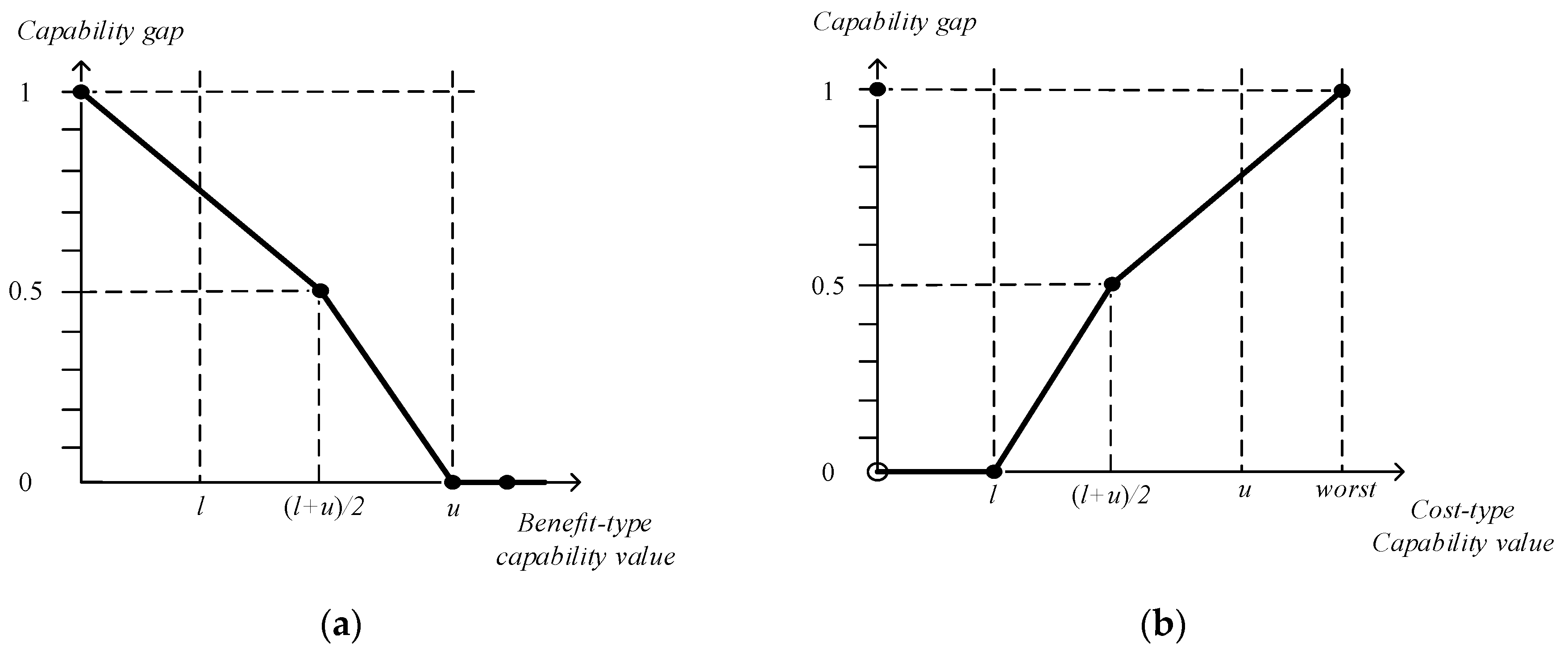
In addition, the capability can be classified into benefit and cost types. Firstly, the relation between a single capability of a solution and corresponding capability requirement is defined based on three premises: (1) When a capability of a solution is deficient or worse than the inferior value of the corresponding capability requirement interval, which means the solution absolutely cannot meet the capability requirement. Its capability gap is supposed to be 1. (2) When a solution can provide a capability, with its value falling in the interval of corresponding capability requirement, its capability gap should be a number between [ 0 , 1 ] . Especially when the solution’s capability value exactly falls in the middle of the capability requirement interval, the capability gap is supposed to be 0.5, which means the capability can meet the capability requirement by half. (3) When a capability of a solution equals to or better than the superior value of the corresponding capability requirement interval, it means that the capability can absolutely meet the corresponding capability requirement, and the capability gap is supposed to be 0.
A concrete case is given in Figure 2, reflecting the relation between a capability and corresponding capability requirement interval [ l , u ] . Four special points discussed above are marked by circle points. To mathematically model the relations with universal forms, a formula is defined to fit the linear line above, shown in Equation (4).
G ( c i , c r i ) = { { c i / ( 2 a ) + 1 , 0 c i < a ( c i + u ) / ( 2 b ) , a c i < u 0 , u < c i ; b e n e f i t t y p e { 1 , c i = 0 0 , 0 < c i < l ( c i l ) / ( 2 b ) , l c i < a ( c i + w o r s t 2 a ) / ( 2 × ( w o r s t a ) ) , a c i < w o r s t ; C o s t t y p e ,
where G ( c i , c r i ) represents the capability gap between the ith capability and corresponding capability requirement interval [ l , u ] . Two special notation a and b are defined to simplify the formula, where a = (l + u)/2, b = (ul)/2. The notation worst denotes the requirement threshold of cost-type capability that the capability gap will be judged to be 1 if a cost-type capability value exceeds worst.
Then, the capability gaps of all capabilities should be aggregated to compute the total capability gap of a system portfolio as i = 1 k w i G ( c i , c r i ) , where the w i denote the weight of the ith capability and is determined according to the method in Section 2.1.1. Then, according to capability gaps, the value is defined as Equation (5), which indicates that the bigger the total capability gap, the smaller the value of a system portfolio.
V ( x j ) = i = 1 k w i ( 1 G ( c i , c r i ) ) k , i = 1 k w i = 1 ,
Different to general “capability-based” evaluation methods, which are usually based on hierarchy structures such as a tree structure that the capabilities of all systems in bottom level are up-aggregated to an integrated value, capability gap is a criterion denoting the gap between capabilities and capability requirements. For general methods, an inevitable defect is that an extremely high capability will pull up the integrated capability value, which is obviously unreasonable. Whereas for the capability gap, it can mitigate the effects of extreme capability values. For example, even an infinitely high benefit-type capability can only result in corresponding capability gap of 0, instead of unreasonably extreme value.

2.2. Risk Decision Based on RUL Prediction

General risk assessment methods follow the steps of risk factor identification, risk analysis, risk assessment and risk management. However, for weapon systems, decision-makers mainly focus on the availability and stability of systems in the operation process. Therefore, the RUL, which denotes when a system is predicted to fault, is used as a weapon system risk criterion. The longer the RUL, the smaller the probability a risk will happen in the operational process. In addition, the RUL prediction method based on similarities of degradation characteristics is proved to perform better than other classical methods when there are sufficient historical samples. Therefore, the paper adopts degradation characteristics similarities to predict the RUL to indicate system portfolio risks.
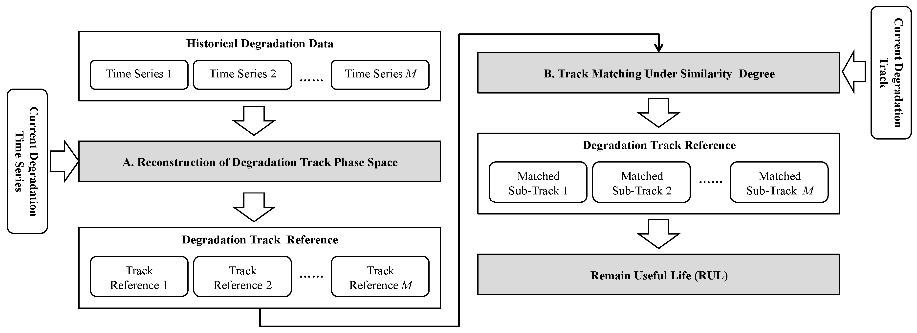
The key resource for predicting RUL is the operational data, which is typically obtained from embedded sensors with time series. In specific, the degradation data is analyzed to support the construction of the RUL prediction model and the main steps can be concluded as degradation track phase space construction, track matching, and RUL prediction. Detailed procedures are given in Figure 3.

2.2.1. Feature extraction based on variation coefficient

When multiple sensors are used to monitor the health of a system, a key step for predicting health states is selecting features from the multidimensional time series data, because only parameters without commonality can be treated as attributes features. Therefore, parameters screening is the prerequisite to ensure the non-commonality of parameters. Intuitively, practitioners should firstly deal with correlations of parameters to make the transformed parameters independent.
In this paper, the statistic of variation coefficients is used to select the parameters features. Similar to the concept of standard deviation and variance in statistics, the variation coefficient is described as the dispersion degree of observations. The variation coefficient is calculated by the ratio of the standard deviation to the mean, as Equation (6) shows. Therefore, it is dimensionless.
V C = ( S t a n d a r d D e v i a t i o n / M e a n ) × 100 % .
Variables with larger variation coefficients show more obvious features and therefore are more suitable for describing characteristics of data.

2.2.2. Reconstruction of Degradation Track Phase Space

According to Taken’s theorem, the potential dynamics laws of a system can be studied by constructing the phase space that preserves the topological properties of the original system. Coupled with the nonlinear characteristics of degradation, the time delay embedding theorem is often applied to construct high-dimensional phase space.
Assume that the time series is X = ( x 1 , x 2 , , x N ) , then the points in the phase space can be expressed as the following form of row vector.
X i = ( x i ( d 1 ) τ , x i ( d 2 ) τ , , x i τ , x i ) , i = 1 + ( d 1 ) τ , 2 + ( d 1 ) τ , , N ,
where d is the embedded dimension of phase space and τ is the time delay.
Embedded dimension d is the key parameter in phase space construction, whose value will be determined by the non-subjective algorithm. X i ( d ) is a point in the d dimension phase space. If the point X n ( i , d ) nearest to X i ( d ) exists, the following relation can be deduced.
X i ( d ) X n ( i , d ) ( d ) = min j = 1 + ( d 1 ) τ , , N , j i X i ( d ) X j ( d ) ,
For all points in the d and d + 1 dimensional phase spaces, the definitions for a ( i , d ) , E ( d ) E ( d ) , E 1 ( d ) , and E 2 ( d ) are given respectively.
a ( i , d ) = X i ( d + 1 ) X n ( i , d + 1 ) ( d + 1 ) X i ( d ) X n ( i , d ) ( d ) E ( d ) = 1 N d τ i = 1 + ( d 1 ) τ N τ a ( i , d ) E 1 ( d ) = E ( d + 1 ) E ( d ) E ( d ) = 1 N d τ i = 1 N τ | x i + d τ x n ( i , d ) + d τ | E 2 ( d ) = E ( d + 1 ) E ( d ) ,
Then the value of the embedded dimension d can be determined by finding the smallest spatial dimension that makes the d and d + 1 dimensional phase spaces topologically equivalent. The topological equivalence here refers to that the nearest neighbors in the d dimensional space still remain the closest in the d + 1 dimensional space, which means that the E 1 ( d ) tends to be a stable value when the d and d + 1 dimensional phase spaces are topologically equivalent. However, in reality, it is difficult to find the smallest d that makes E 1 ( d ) a stable value. That’s why the E ( d ) and E 2 ( d ) are defined. If x is a random time series, then E 2 ( d ) will vary with d, or E 2 ( d ) will approach 1. Then by combining E 1 ( d ) and E 1 ( d ) , the embedded dimension of the degradation track phase space can be determined. After the construction of the phase space, the time series can be transformed into the form of special track. By referring to the degradation data transformed from historical data and comparing the similarity of the new track with the reference track in phase space, the RUL can be predicted.

2.2.3. System Portfolio Risk Determination Based on RUL

Assume that Z = { Z 1 , Z 2 , , Z l 1 } represents the degradation reference track and Y = { Y 1 , Y 2 , , Y l 2 } , l 1 > l 2 , is the current degradation track. Then, the normalized cross correlation (NCC) is introduced to measure the similarity between tracks. The specific definition of NCC is given as follows:
s Y Z ( i ) = ( Y Y ¯ ) × ( Z i Z ¯ i ) Y Y ¯ 2 Z i Z ¯ i 2 ,
where Z i = { Z i , Z i + 1 , , Z i + l 2 1 } and Y are of the same length. Y ¯ and Z ¯ i are the mean vectors of Y and Z i respectively.
Taking the jth time series x j = { x 1 j , x 2 j , , x N j j } as an example, the time points of the time series are denoted as t j = { t 1 j , t 2 j , , t N j j } . Apparently, t N j j is the running life of the j th degradation process. Taking time delay τ as 1 and considering embedded dimension as d for all degradation track phase spaces (d is no less than the maximal embedded dimension of all phase spaces). Then the original time series of degradation process is transformed into the track of phase space. Denoting the reference track for the jth process as Z j = [ X d j , X d + 1 j , , X N j j ] T , the points in phase space are expressed as X i j = [ x i ( d 1 ) j , x i ( d 1 ) j , x i j ] .
Assuming the current degradation time series is y = { y 1 , y 2 , , y c } . Similarly, it is transformed into an incomplete degradation track form denoted as Y = [ Y d , Y 1 + d , , Y c ] , Y i = [ y i ( d 1 ) , y i ( d 2 ) , , y i 1 , y i ] .
When performing track matching, a track subset Y k = [ Y k l + 1 , , Y k ] is selected with a time window length of l in the current phase space. Then the NCC between the current track Y k and the reference track Z j should be modified as follows.
s k j = s Y Z + ( 1 | t k t k j | t k ) ,
If the s k j reaches the maximum at the time point T k j , then sub-tracks at time T k j are regarded as the best matching results in terms of degradation reference track Z j . This result also reflects the influence of the track shape to the degradation stage. Therefore, the RUL of the most similar part to the jth degradation reference track can be estimated as L k j = t N j j T k j .
On the basis of the above result of the best track matching, the weight of the remaining life calculated according to the jth degradation reference track is given as w k j = s k j ( T k j ) / ( j = 1 M s k j ( T k j ) ) , where M is the total number of the degradation processes. Then the remaining life of the system k is estimated as Equation (12).
R U L k = j = 1 M ω k j L k j ,
Then, the RUL should be transformed into risk according to the joint probability. It is identified as a risk event when any system in a system portfolio breaks. Therefore, for a system portfolio x i = ( s 1 , s 2 , , s n ) , the risk is calculated as Equation (13) shows.
R ( x i ) = 1 j = 1 n [ ( 1 1 R U L j ) x i j ] ,
In conclusion, the RUL is an important criterion for the weapon system research because longer RUL can reduce the failure risk of systems in combat. The availability of each component system is the basis to guarantee the normal operation of systems portfolios. An operation activity will be broken or even unsuccessful if any system of a system portfolio malfunctions in the operation process. This induces the demand for long RUL of systems.

2.3. System Portfolio Optimization

As discussed above, the paper tries to solve the system portfolio problem considering system values and risks. The corresponding notation is as follows. Let S = { s 1 , , s m } denotes the set of alternative systems, indicating m systems can be selected for a system portfolio. x i = ( x i 1 , , x i m ) , x i { 0 , 1 } m is one of system portfolio schemes, where x i j = 0 \ 1 , with x i j = 0 denoting the jth system in S is not selected in scheme x i , and x i j = 1 denoting the jth system in S is selected in scheme x i . All possible schemes compose the solution space X. Let E = ( e 1 , , e m ) represents the cost of systems, where e i is the cost of system s i , and B denotes the total budget.
Then, the system portfolio optimization model can be formulated as follows.
m a x V ( x j ) = i = 1 k w i ( 1 G ( c i , c r i ) ) k m i n R ( x j ) = 1 i = 1 k [ ( 1 1 R U L i ) x j i ] s . t . { i = 1 m x j i × e i B x j = ( x j 1 , , x j m ) , x j { 0 , 1 } m ,
where V ( x j ) and R ( x j ) are the value and risk of the system portfolio scheme x j . G ( c i , c r i ) represents the capability gap on the ith capability. In addition, the cost of scheme x j must within the budget limitation.
It can be seen that the optimization is a multi-objective problem and the 2 objectives are conflict with each other. Therefore, an optimal system portfolio with the best performance in both 2 objectives does not exist. The target is to obtain the Pareto optimal solutions of 2 objectives, also known as non-dominated solutions.

3. Results

3.1. Background Description

It is hypothesized that the problem aims to select an optimal system portfolio under the anti-missile scenario, where an object will suffer saturated missiles attacks. The objective is selecting a system portfolio from 100 alternative systems ( 2 100 1 candidate system portfolios in total) under the budget limitation to maximize the system portfolio value and simultaneously minimize the whole risk.
According to the operation process of OODA, capabilities discussed in the paper are c 1 detection range, c 2 communication range, c 3 striking range and c 4 decision time, where the former three capabilities are beneficial type and the last one is cost type. In a specific operation scenario, the capability requirements and combination rules are shown in Table 1.
In addition, for capabilities of systems, they are generated by executing a Monte Carlo simulation method according to truncated normal distribution functions. The histogram of generated data is shown in Figure 4. The worst value of cost-type capability decision time is 34.6853, which will be used in value calculation according to Section 2.1.2.

3.2. Value Calculation

3.2.1. Weight Determination

Based on simulations on the “Command: Modern Air/Naval Operations”, an ultimate military simulator for modern military conflicts, the weight information can be deduced by the correlation analysis.
The independent variables are four capabilities, that is detection range, communication range, striking range and decision time. The dependent variable is the intercepted missile number. By auto-simulating for 10,000 times, 10,000 sets of data are generated. Through the MIC algorithm, the corresponding results can be obtained, as Table 2 shows. Through normalization, the weight of four capabilities are determined as 0.276, 0.250, 0.174, and 0.300.

3.2.2. Value Calculation

Because it is impossible to calculate all values of 2 100 1 candidate system portfolios, an example of the value calculation process is introduced. Assuming a system portfolio SP1 have 5 component systems of S1, S2, S3, S4, and S5, with capability information shown in Table 3.
According to capability combination rules in Table 1, the combined capabilities of system portfolio SP1 are shown in the last column in Table 3.
Then, according to Equation (4), the capability gaps of four combined capabilities are calculated as Equation (15) shows. The value of any system portfolio can be calculated based on the same steps.
G ( c 1 , C r 1 ) = 0 G ( c 1 , C r 1 ) = ( 150.0713 100 + 250 ) + 1 = 0.571 G ( c 1 , C r 1 ) = ( 218.758 150 + 300 ) + 1 = 0.514 G ( c 1 , C r 1 ) = ( 18.44034 10 30 10 ) = 0.422 ,

3.3. Risk Determination Based on RUL Prediction

In the case study, the key component of weapon systems, the turbine engine, is taken as an example for analyzing risks. The data is derived from the experiment conducted by a commercial modular simulation software C-MAPSS as shown in Figure 5.
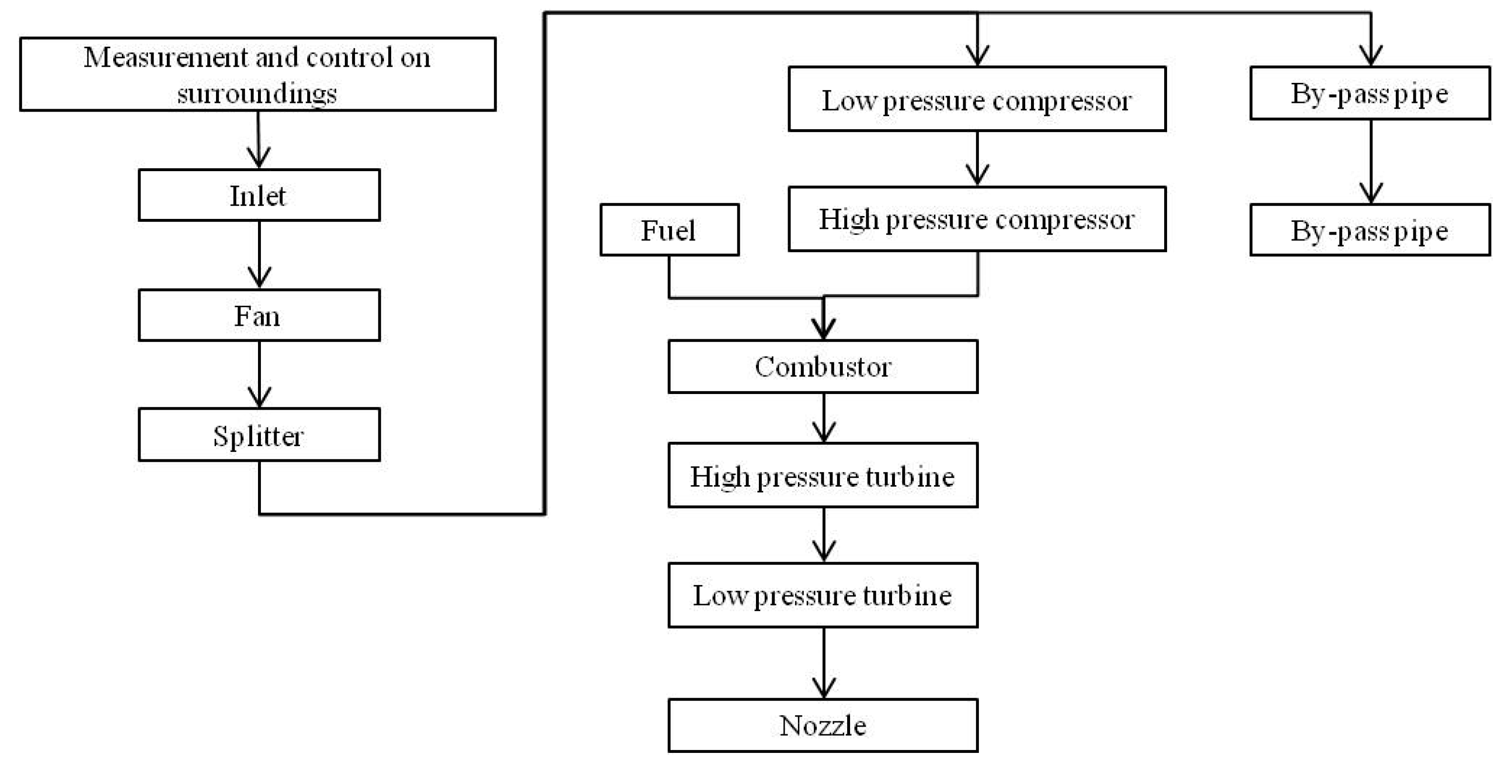
The C-MAPSS simulates the operation of a turbine engine with 900,000-pound thrust and records monitoring signals. Based on the principle of thermodynamics, two failure modes are designed: high-pressure compressor degradation and fan degradation. The main functional modules and connections are shown in Figure 6. The simulation runs in the following settings:
(1)
The simulation experiment data contains time series of 21 variables. It can be further divided into a training set and a testing set. Each multivariate time series corresponds to a specific engine, meaning that the data can be considered to be generated by engines of different systems.
(2)
The initial wear condition of each engine might not be identical and there are manufacturing variations, which are considered reasonable and not treated as reasons of engine failures.
(3)
There are 3 operational setting parameters that have a substantial impact on an engine’s performance.
(4)
There are noises in the data.
(5)
The engines operate normally at the initial moment and begin to degrade at some points in time series. In the training set, the cumulative degradation quantity continues to grow until it reaches or exceeds the preset threshold. In the testing set, the time series will terminate when engines fail.
As a result, 100 degradation tracks are obtained in the training set and 100 tracks before failure in the testing set. The training data is used to establish the RUL prediction model of engines, and the testing set is used to test the feasibility of the model.
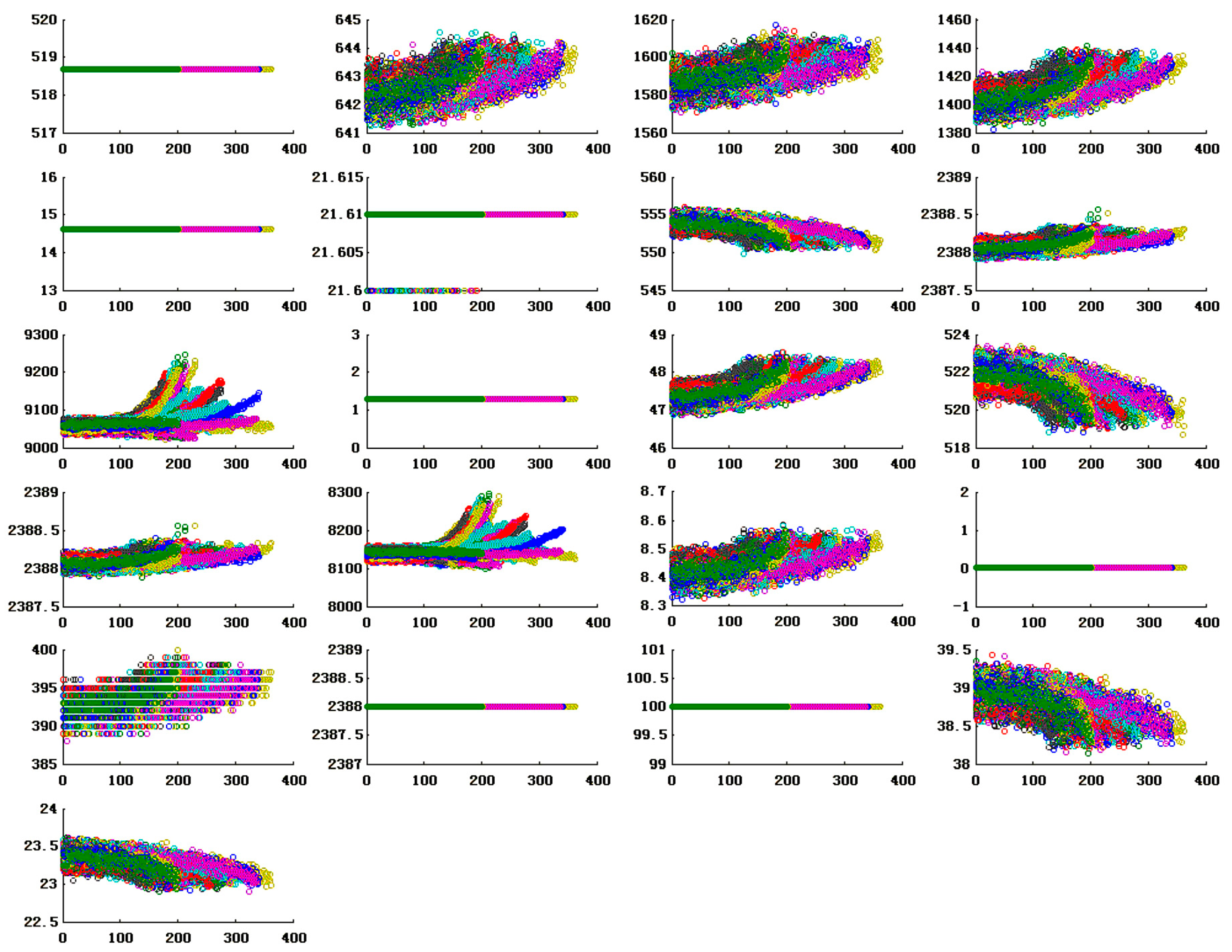
The monitoring data is shown in the scatter plots in Figure 7. Each plot visualizes the 100 degradation tracks of one variable in the training set. The engine code, the operation cycle and the 3 operational setting parameters are not shown in the figure.
Due to the fact that the constant variable is unable to reflect the evolution of engine degradations, variable 1, 5, 6, 10, 16, 18, and 19 are not regarded as feature variables. What’s more, the tracks exhibit different trends in terms of variable 9 and 14, so variable 9 and 14 are inadequate to describe the degradation process.
Then, the variation coefficients of the rest 12 variables are calculated based on the degradation data and the results are shown in Table 4. According to the rule of eliminating variables with small variation coefficients, variable 3, 4, 11, 15, 17, 20 and 21 are chosen as the base variables that represent engine degradation characters.
According to the RUL prediction method, the remaining life of the engines in the testing set can be estimated by matching the testing data with the reference tracks. Then, the risks can be obtained. The results are shown in Table 5.

3.4. Portfolio Selection Results Analysis

In total, there are 2 100 1 possible schemes, which is a huge number. Thus, a heuristic algorithm is necessary to be applied to the solving process. Considering the value and risk factors, the objectives are maximizing the value and minimize the risk of system portfolios. Therefore, a multi-objective algorithm is employed to solving the optimization problem. The non-dominated sorting generic algorithm (NSGA) is a kind of widely used multi-objective algorithm, which exhibits a good performance for retaining elites in offspring. On the other side, the differential evolution (DE) is a nice genetic operator, which plays really well on keeping population diversity. Thus, the paper uses the non-dominated differential evolution (NSDE) algorithm, which fuses the two advantages of NSGA and DE, to solve the system portfolio optimization problem. The corresponding parameters are set as follows. The population size is Pop = 100, the number of iterations is Gen = 1000, the mutation probability is 0.01 and the crossover probability is 0.2.
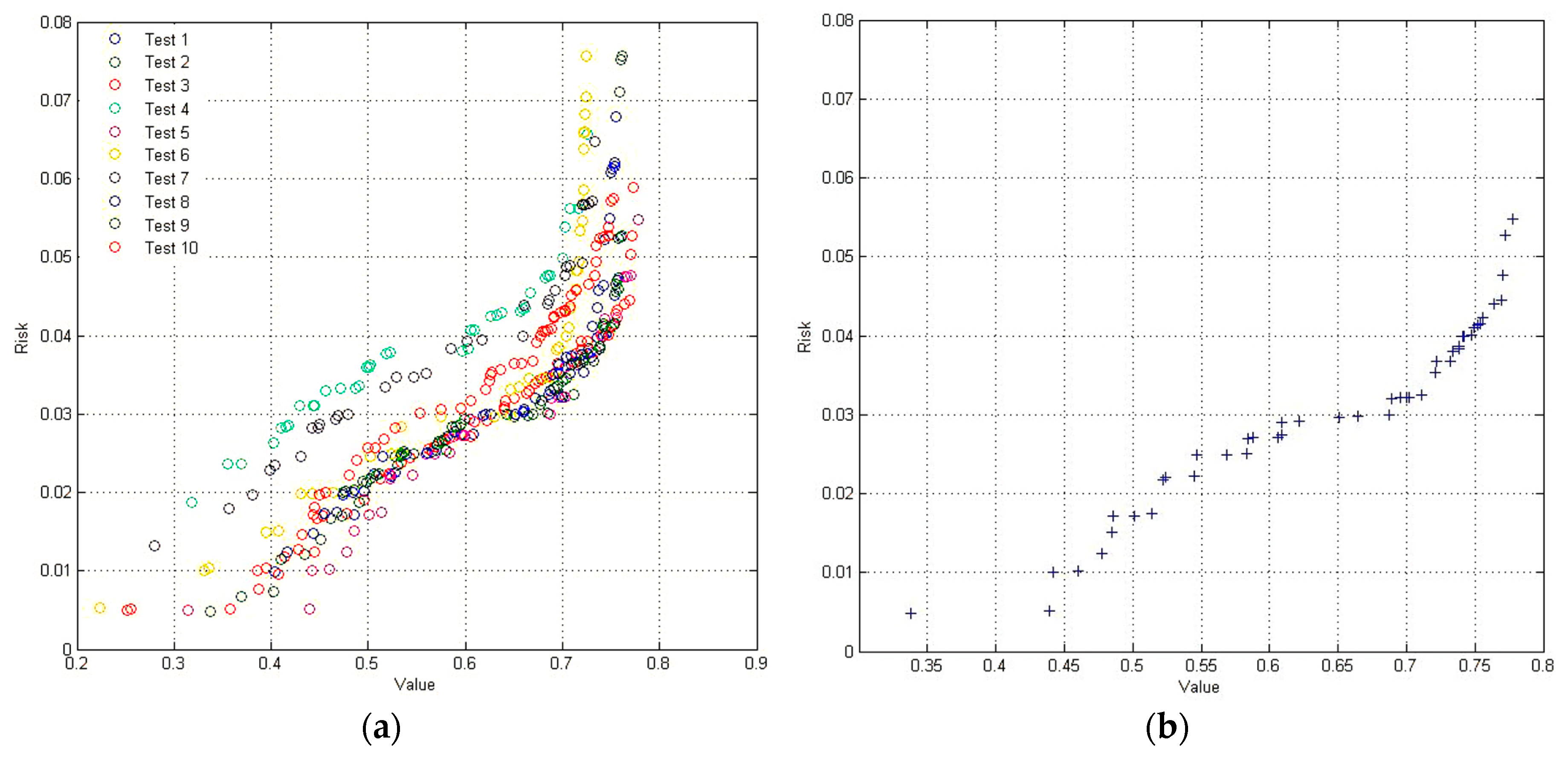
Due to the certain randomization of all genetic algorithms, The NSDE also generates results with certain fluctuant. A typical method to guarantee the optimality of generated result is running the algorithm for multiple times, and then select the best individuals by comparing the corresponding multiple results. In the case, the program is iterated for 10 times to generate 10 Pareto results with each containing 200 individuals, shown in (a) of Figure 8. Then, the 10 sets of Pareto results are combined together to obtain the best 200 individuals among them, as shown in (b) of Figure 8.
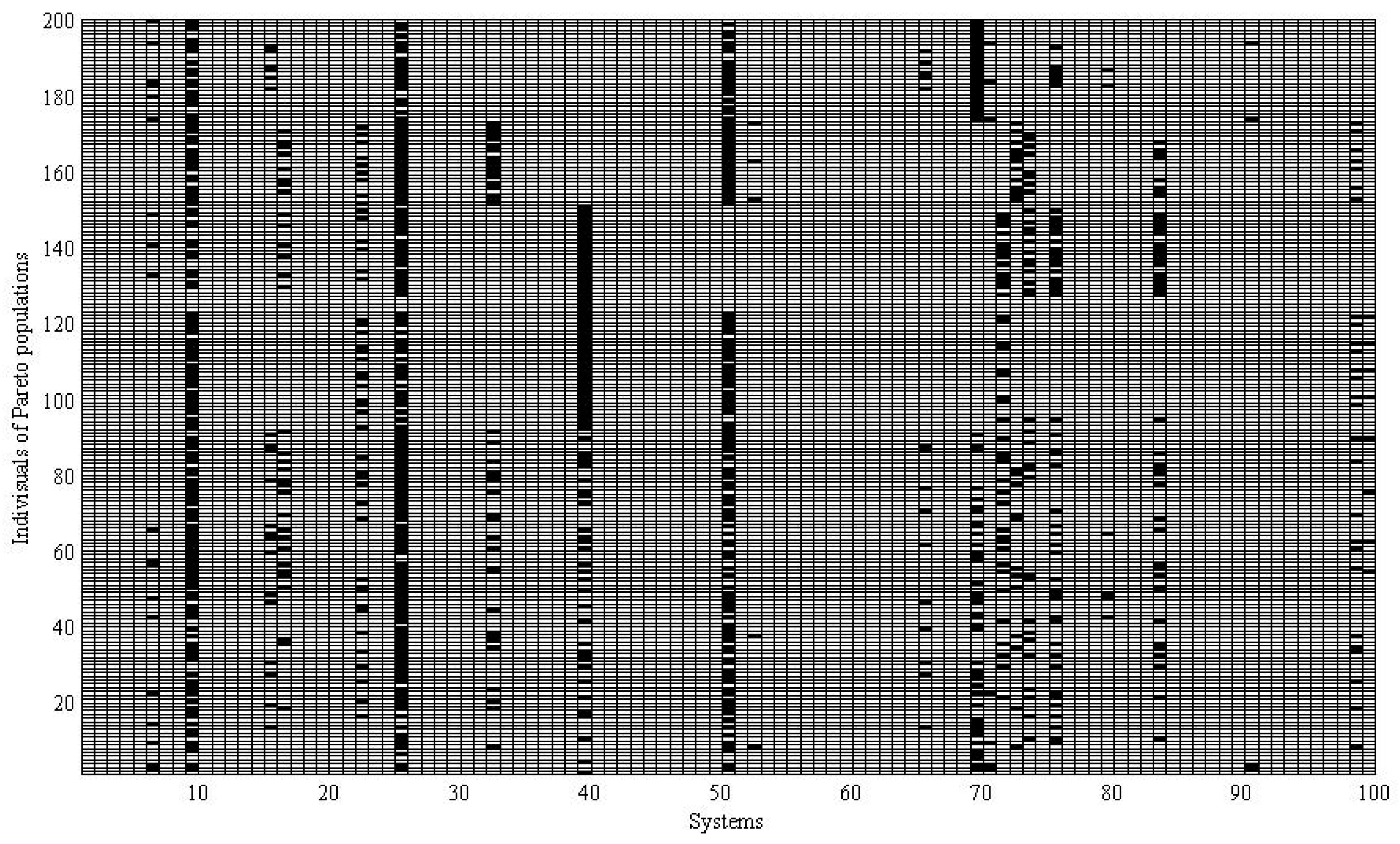
In detail, the 200 individuals of the best Pareto set are shown in the system option diagram in Figure 9. The rectangular area is divided into 100 × 200 rectangles according to the number of system candidates and the dimension of the non-dominated weapon system portfolios. Each rectangle represents whether a system candidate is selected in the Pareto set. If a weapon system i is selected by the j th non-dominated system portfolio, the i th row and j th column rectangular block will be colored black, otherwise, it is left blank.
From Figure 10, it can be seen that some systems are frequently selected in the Pareto set. However, some systems are seldom selected or even never selected. To compare the importance degree of different systems, the frequencies for all systems of being selected in the Pareto set is counted. Systems of S6, S9, S15, S16, S22, S25, S32, S39, S50, S52, S65, S69, S70, S71, S72, S73, S75, S79, S83, S90, S98, and S99 are selected by at least one system portfolio in the Pareto set. In addition, the systems S9, S25, S50 are quite important according to the high selected numbers in the Pareto set. Further, the rank of systems according to selected numbers is: S25 > S9 > S50 > S39 > S69 > S75 > S83 > S22 > S71 > S32 > S73 > S16 > S98 > S72 > S15 > S6 > S65 > S99 > S70 > S79 > S52 > S90, which to some extend indicates the importance degrees of selected systems. As regarding to the rest systems, they can be directly neglected in the system portfolio selection process.
By deeper analysis, it can be discovered that some systems tend to always be selected together. Therefore, a frequent item set mining algorithm of Apriori is applied to identify the association rules, shown in Table 6. The support parameter indicates the ratio between the simultaneously appearing frequency and all items, which means the probability of appearing simultaneously. The confidence of the rule of “A B” represents the ratio of s u p p o r t ( A B ) / s u p p o r t ( A ) , which means the probability of A B when A appears.
In Table 5, the association rules are ranked by the value of support and confidence respectively. Firstly, according to the ranking by support, it can be elicited that the “S9 S25” is the most frequent rule, which means they tend to be selected together. In addition, when system S75 is selected, the system S25 must also be selected according to the first rule in the ranking by confidence. Referring the association rules, decision-makers can have a deeper understanding of the significance of system portfolios.

4. Discussion

The paper shows the feasibility of replacing expert subjective expertise with knowledge obtained from data. Firstly, the weight information of capabilities is determined by analyzing correlations between capabilities and the intercepted missile numbers, based on operation simulation data. Then, as regards the risk criterion, the paper tries to determine the risk by mining information from system operation data. The data-driven methods are only components of the model-based approaches, aiming to increase the accuracy and credibility of results.
In the case study, 100 system candidates are provided to be optimized on the scenario of anti-missile. By automatically simulating the operation scenario for 10,000 times, 10,000 simulation results are generated, according to which, the maximal information coefficients between four capabilities and the variable of intercepted missile quantity are calculated as the weight of capabilities. It quantitatively indicates that the capability of decision time has the biggest impact on the interpreted missile quantity. In addition, by running the simulator of C-MAPSS for 200 times, 200 groups of system operation data are generated, according to which, systems risks are obtained through prediction of RUL.
In the system portfolio optimization, considering the great number of 2 100 1 candidate system portfolios, the NSDE algorithm is applied to solving the optimization problem. To guarantee the optimality of the result as far as possible, 10 Pareto sets are obtained by running the NSDE for 10 times. 200 non-dominated individuals are reserved by comparing the 10 Pareto sets. However, it can be not proved the best Pareto set, due to the almost infinity of candidate system portfolios and the randomness of genetic algorithms. By further analyzing the characters of generated Pareto set, 22 systems are selected at least one time, and 16 association rules are mined. These characters can play an assistant rule for decision-makers to make a deeper understanding of the system portfolios.
In conclusion, the system portfolio selection is the mainstream trend of future equipment development. Compared to other traditional system portfolio decision and optimization methods, the proposed model and data-driven approach provide a solution to avoid the excessive dependence on subjective expert experience in the evaluation and decision process. Traditionally, determining these parameters requires cumbersome processes of organizing experts, collecting expert opinions, analyzing expert scores etc., which are time and effort-consuming and more likely to be questioned. The model and data-driven methods can make use of models that have been proved to be effective on one hand, and on the other hand, it can determine the required parameter values in the model through data analysis. Therefore, it supports more efficient, more credible, and more practical evaluation and decisions in system portfolio selection and other fields applications.

Author Contributions

H.W. wrote the main parts of the paper; B.X. and Z.Z. designed and performed the simulations in the case study; Z.Y. and Z.Z. analyzed the result.

Funding

The work was funded by the National Natural Science Foundation of China, Grant 71690233 and 71571186.

Acknowledgments

We thank the C-MAPSS developers and the National Aeronautics and Space Administration (NASA) for providing the engine simulation data inputs.

Conflicts of Interest

The authors declare no conflict of interest.

References

  1. Xia, B.; Dou, Y.; Zhao, Q.; Ge, B.; Zhang, Y. Robust System Portfolio Selection with Multi-Function Requirements and System Instability. In Proceedings of the Proceedings of the Systems Conference (SysCon), Montreal, QC, Canada, 24–27 April 2017. [Google Scholar]
  2. Markowitz, H. Portfolio selection. J. Financ. 2012, 7, 77–91. [Google Scholar]
  3. Ľuboš, P. Portfolio Selection and Asset Pricing Models. J. Financ. 2000, 55, 179–223. [Google Scholar]
  4. Mohagheghi, V.; Mousavi, S.M.; Vahdani, B.; Shahriari, M.R. R&D project evaluation and project portfolio selection by a new interval type-2 fuzzy optimization approach. Neural Comput. Appl. 2017, 28, 3869–3888. [Google Scholar]
  5. Abdollahi, M.; Arvan, M.; Razmi, J. An integrated approach for supplier portfolio selection: Lean or agile. Expert Syst. Appl. 2015, 42, 679–690. [Google Scholar] [CrossRef]
  6. McCarthy, D.M. One Size Does Not Fit All-Right-Sized Signal Detection Systems That Are Appropriate for Your Portfolio Benefit-Risk Management Strategy. Pharmacoepidemiol. Drug Saf. 2016, 25, 404–405. [Google Scholar]
  7. Achillas, C.; Aidonis, D.; Iakovou, E.; Thymianidis, M.; Tzetzis, D. A methodological framework for the inclusion of modern additive manufacturing into the production portfolio of a focused factory. J. Manuf. Syst. 2015, 37, 328–339. [Google Scholar] [CrossRef]
  8. Dou, Y.; Zhang, P.; Ge, B.; Jiang, J.; Chen, Y. An integrated technology pushing and requirement pulling model for weapon system portfolio selection in defense acquisition and manufacturing. Proc. Inst. Mech. Eng. B J. Eng. 2015, 229, 1046–1067. [Google Scholar] [CrossRef]
  9. Chien, C.F.; Huynh, N.T. An Integrated Approach for IC Design R&D Portfolio Decision and Project Scheduling and a Case Study. IEEE Trans. Semiconduct. Manuf. 2018, 31, 76–86. [Google Scholar]
  10. Liesio, J.; Salo, A. Scenario-based portfolio selection of investment projects with incomplete probability and utility information. Eur. J. Oper. Res. 2012, 217, 162–172. [Google Scholar] [CrossRef]
  11. Li, Y.P.; Huang, G.H.; Chen, X. Multistage scenario-based interval-stochastic programming for planning water resources allocation. Serra 2009, 23, 781–792. [Google Scholar] [CrossRef]
  12. Xia, B.; Zhao, Q.; Yang, K.; Dou, Y.; Yang, Z. Scenario-Based Modeling and Solving Research on Robust Weapon Project Planning Problems. J. Syst. Eng. Electron. 2019, 30, 85–99. [Google Scholar]
  13. Rafiee, M.; Kianfar, F. A scenario tree approach to multi-period project selection problem using real-option valuation method. Int. J. Adv. Manuf. Tech. 2011, 56, 411–420. [Google Scholar] [CrossRef]
  14. Ben-Tal, A.; Chung, B.D.; Mandala, S.R.; Yao, T. Robust optimization for emergency logistics planning: Risk mitigation in humanitarian relief supply chains. Transp. Res. B Meth. 2011, 45, 1177–1189. [Google Scholar] [CrossRef]
  15. Ismail, A.; Pham, H. Robust Markowitz mean-variance portfolio selection under ambiguous covariance matrix. Math. Financ. 2019, 29, 174–207. [Google Scholar] [CrossRef]
  16. Hu, J.; Mehrotra, S. Robust and stochastically weighted multi-objective optimization models and reformulations. Oper. Res. 2012, 60, 939–953. [Google Scholar] [CrossRef]
  17. Quintana, D.; Denysiuk, R.; Garcia-Rodriguez, S.; Gaspar-Cunha, A. Implementation Risk Management Using Evolutionary Multiobjective Optimization. Appl. Sci. 2017, 7, 1079. [Google Scholar] [CrossRef]
  18. Poklepović, T.; Marasović, B.; Aljinović, Z. Portfolio selection model-based on technical, fundamental and market value analysis. In Proceedings of the European Conference on Operational Research, Vilnius, Litva, 8–11 July 2012. [Google Scholar]
  19. Liesiö, J.; Mild, P.; Salo, A. Robust portfolio modeling with incomplete cost information and project interdependencies. Eur. J. Oper. Res. 2008, 190, 679–695. [Google Scholar] [CrossRef] [Green Version]
  20. Golabi, K.; Kirkwood, C.W.; Sicherman, A. Selecting a portfolio of solar energy projects using multi-attribute preference theory. Manag. Sci. 1981, 27, 174–189. [Google Scholar] [CrossRef]
  21. Ge, B.; Hipel, K.W.; Fang, L.; Yang, K.; Chen, Y. An Interactive Portfolio Decision Analysis Approach for System-of-Systems Architecting Using the Graph Model for Conflict Resolution. IEEE Trans. Syst. Man Cybern. Syst. 2014, 44, 1328–1346. [Google Scholar] [CrossRef]
  22. Beraldi, P.; Violi, A.; Ferrara, M.; Ciancio, C.; Pansera, B.A. Dealing with complex transaction costs in portfolio management. Ann. Oper. Res. 2019. [Google Scholar] [CrossRef]
  23. Saborido, R.; Ruiz, A.B.; Bermúdez, J.D.; Vercher, E.; Luque, M. Evolutionary multi-objective optimization algorithms for fuzzy portfolio selection. Appl. Soft. Comput. 2016, 39, 48–63. [Google Scholar] [CrossRef]
  24. Nalpas, N.; Simar, L.; Vanhems, A. Portfolio selection in a multi-moment setting: A simple Monte-Carlo-FDH algorithm. Eur. J. Oper. Res. 2017, 263, 308–320. [Google Scholar] [CrossRef]
  25. Sands, C. Application of Multi-Criteria Decision Making Methods to the DLA Energy Military Construction Portfolio Selection Process. Ph.D. Thesis, Washington, DC, USA, 2016. [Google Scholar]
  26. Yang, S.; Yang, M.; Wang, S.; Huang, K. Adaptive immune genetic algorithm for weapon system portfolio optimization in military big data environment. Cluster Comput. 2016, 19, 1359–1372. [Google Scholar] [CrossRef]
  27. Kangaspunta, J.; Liesiö, J.; Salo, A. Cost-efficiency analysis of weapon system portfolios. Eur. J. Oper. Res. 2012, 223, 264–275. [Google Scholar] [CrossRef]
  28. Greiner, M.A.; Mcnutt, R.T.; Shunk, D.L.; Fowler, J.W. Selecting military weapon systems development portfolios: Challenges in value measurement. In Proceedings of the Portland International Conference on Management of Engineering & Technology, Portland, OR, USA, 29 July–2 August 2001. [Google Scholar]
  29. Cheng, C.; Li, J.; Zhao, Q.; Jiang, J.; Yu, L.; Shang, H. Research on weapon system portfolio selection based on combat network modeling. In Proceedings of the Systems Conference (SysCon), Montreal, QC, Canada, 24–27 April 2017. [Google Scholar]
  30. Zhou, Z.; Dou, Y.; Xia, B.; Jiang, J. Weapon systems portfolio selection based on fuzzy clustering analysis. In Proceedings of the IEEE International Conference on Control Science & Systems Engineering, Beijing, China, 17–19 August 2017. [Google Scholar]
  31. Li, M.H.; Li, M.J.; Yang, K.W.; Xia, B.Y.; Wan, C.Q. A Network-Based Portfolio Optimization Approach for Military System of Systems Architecting. IEEE Access 2018. [Google Scholar] [CrossRef]
  32. Yu, Z.; Tan, Y.J.; Yang, K.W.; Yu, Z.Y. Research on evolving capability requirements oriented weapon system of systems portfolio planning. In Proceedings of the International Conference on System of Systems Engineering, Genova, Italy, 16–19 July 2012. [Google Scholar]
  33. Huang, K. Combinatorial optimization and simulation for weapon system portfolio using self-adaptive Memetic algorithm. J. Eng. Res. 2017, 5, 124–139. [Google Scholar]
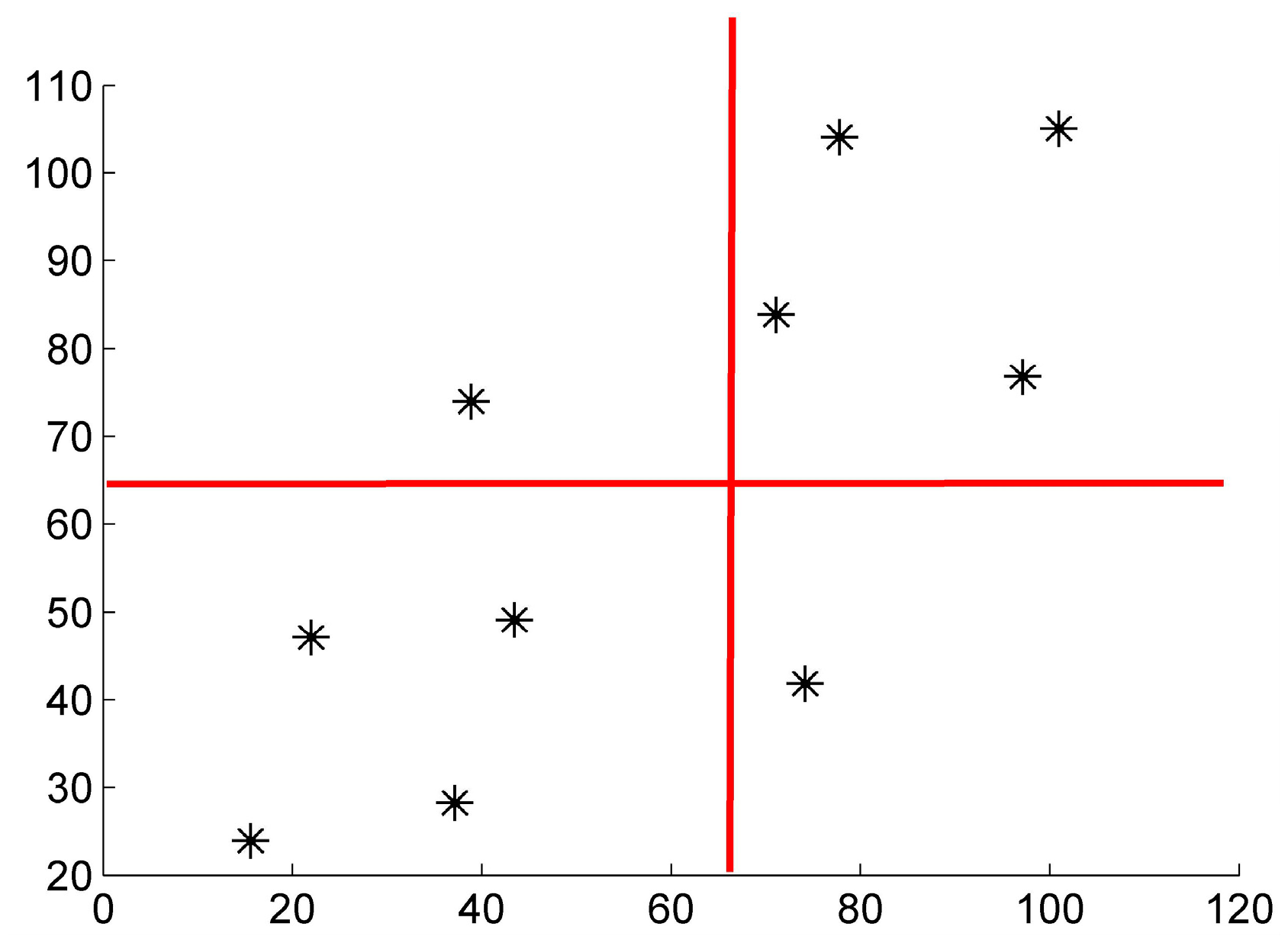
Figure 1. Division for variable X and Y.
Applsci 09 01657 g001
Figure 2. The gap function curve: (a) Benefit type capability, (b) cost type capability.
Applsci 09 01657 g002
Figure 3. RUL prediction procedures.
Applsci 09 01657 g003
Figure 4. Histogram of generated capability data.
Applsci 09 01657 g004
Figure 5. The interface of the simulation platform.
Applsci 09 01657 g005
Figure 6. The functional modules and their connection.
Applsci 09 01657 g006
Figure 7. Scatter plots of the time series in terms of the different monitoring signals.
Applsci 09 01657 g007
Figure 8. Result exhibition: (a) Result of 10 times of running; and (b) result of 200 best individuals.
Applsci 09 01657 g008
Figure 9. System option diagram.
Applsci 09 01657 g009
Figure 10. Frequencies for all systems of being selected in the Pareto set.
Applsci 09 01657 g010
Table 1. Capabilities requirements.
Capabilities c 1   ( Km ) c 2   ( Km ) c 3   ( Km ) c 4   ( Second )
CR[100,200][100,250][150,300][10,30]
RulesMaximalAdditionAdditionAverage
Table 2. Obtained maximal information coefficient (MIC) of input and output.
MICIntercepted Missile Number
Detection range0.854
Communication range0.772
Striking range0.537
Decision time0.928
Table 3. Capabilities of 5 systems.
SystemsDetection RangeCommunication RangeStriking RangeDecision Time
S1128.850201845.0022155941.9362617122.55909356
S2205.160469336.3594850450.0154132316.53053513
S3156.960028727.1132984643.2835739916.46184426
S4152.712094326.1907193553.5711512721.31900886
S5111.517014715.4055380429.9516114515.33123079
SP1205.1604693150.0713218.75818.44034
Table 4. Variation coefficients (VC) of the rest 12 variables.
VariableSensor 2Sensor 3Sensor 4Sensor 7Sensor 8Sensor 11Sensor 12Sensor 13Sensor 15Sensor 17Sensor 20Sensor 21
VC0.05670.27600.51100.12390.00200.45730.11170.00200.34080.29070.35190.3514
Table 5. The prediction results of the remaining life of different weapon systems.
SRULRiskSRULRiskSRULRiskSRULRisk
S11120.008929S261970.005076S511140.008772S76760.013158
S21040.009615S271620.006173S52720.013889S77780.012821
S3970.010309S28820.012195S53780.012821S781990.005025
S4920.01087S29750.013333S541870.005348S791670.005988
S51330.007519S30830.012048S551890.005291S801090.009174
S61050.009524S31750.013333S56750.013333S81750.013333
S7810.012346S321500.006667S57760.013158S82750.013333
S8610.016393S331210.008264S58750.013333S832020.00495
S91370.007299S34750.013333S591900.005263S84740.013514
S10660.015152S35740.013514S60870.011494S851620.006173
S111070.009346S36750.013333S61720.013889S861560.00641
S121070.009346S37990.010101S62680.014706S872030.004926
S13790.012658S38760.013158S63670.014925S881260.007937
S141360.007353S392080.004808S64740.013514S89790.012658
S151970.005076S40740.013514S652000.005S90790.012658
S161880.005319S41940.010638S66740.013514S91720.013889
S17790.012658S42730.013699S672000.005S92750.013333
S181010.009901S43790.012658S68750.013333S93690.014493
S191710.005848S441850.005405S691970.005076S94790.012658
S20750.013333S45780.012821S70870.011494S951870.005348
S211560.00641S46820.012195S712020.00495S961890.005291
S221820.005495S471190.008403S721300.007692S971760.005682
S231820.005495S481630.006135S731900.005263S981210.008264
S24750.013333S49280.035714S741170.008547S991890.005291
S252030.004926S501950.005128S751950.005128S100730.013699
Table 6. The association rules mined by frequent item set mining.
Ranking by SupportRanking by Confidence
Association RulesSupportConfidenceAssociation RulesSupportConfidence
9 250.6150.872375 250.2551.0000
25 90.6150.7593[9,39] 250.280.9032
50 250.570.8906[9,50] 250.4650.9029
25 500.570.703750 250.570.8906
50 90.5150.80479 250.6150.8723
9 500.5150.7305[25,50] 90.4650.8158
[9,50] 250.4650.902950 90.5150.8047
[25,50] 90.4650.8158[25,39] 90.280.7887
[9,25] 500.4650.756125 90.6150.7593
50 [9,25]0.4650.7266[9,25] 500.4650.7561
9 [25,50]0.4650.659669 500.250.7353
[9,39] 250.280.90329 500.5150.7305
[25,39] 90.280.788750 [9,25]0.4650.7266
39 [9,25]0.280.622225 500.570.7037
75 250.2551.00009 [25,50]0.4650.6596
69 500.250.735339 [9,25]0.280.6222