Article

An Intelligent Hybrid Energy Management System for a Smart House Considering Bidirectional Power Flow and Various EV Charging Techniques

by
Muhammad Kashif Rafique
1,
Saad Ullah Khan
2,
Muhammad Saeed Uz Zaman
1,
Khawaja Khalid Mehmood
3,
Zunaib Maqsood Haider
4,
Syed Basit Ali Bukhari
1 and
Chul-Hwan Kim
1,*
1
Department of Electrical and Computer Engineering, Sungkyunkwan University, Suwon 16419, Korea
2
Department of Electrical and Computer Engineering, Air University, Islamabad 44000, Pakistan
3
U.S.-Pakistan Center for Advanced Studies in Energy (USPCAS-E), National University of Sciences and Technology (NUST), H-12 Campus, Islamabad 44000, Pakistan
4
Department of Electrical Engineering, NFC Institute of Engineering and Technology, Multan 60000, Pakistan
*
Author to whom correspondence should be addressed.
Appl. Sci. 2019, 9(8), 1658; https://doi.org/10.3390/app9081658
Submission received: 12 March 2019 / Revised: 14 April 2019 / Accepted: 15 April 2019 / Published: 22 April 2019
(This article belongs to the Special Issue Smart Home and Energy Management Systems 2019)

Abstract

:
Compelled by environmental and economic reasons and facilitated by modern technological advancements, the share of hybrid energy systems (HES) is increasing at modern smart house (SH) level. This work proposes an intelligent hybrid energy management system (IHEMS) for an SH connected to a power network that allows a bidirectional power flow. The SH has electrical and thermal power loops, and its main components include renewable energy from wind and photovoltaics, electric vehicle (EV), battery energy storage system, a fuel cell which serves as a micro-combined heat and power system, and a boiler. The proposed IHEMS models the components of the SH, defines their constraints, and develops an optimization model based on the real coded genetic algorithm. The key features of the developed IHEMS are highlighted under six simulation cases considering different configurations of the SH components. Moreover, the standard EV charging techniques are compared, and it is observed that the charging method which is flexible in timing and power injection to the EV is best suited for the economic operation of the SH. The simulation results reveal that the proposed IHEMS minimizes the 24-hour operational cost of the SH by optimally scheduling the energy resources and loads.

1. Introduction

1.1. Background and Motivation

The contribution of hybrid energy systems (HES) is increasing in the world at industrial, commercial, and domestic levels to address environmental and economic concerns [1]. A HES consists of two or more energy resources operated together to obtain an improved efficiency and a better energy balance. Due to advanced technology, compact and high-efficiency micro-combined heat and power systems (micro-CHP) are gaining popularity at domestic level [2,3,4,5,6,7]. According to the American Council for an Energy-Efficient Economy’s report, the modern CHP systems can work at an efficiency as high as 80% in contrast to the commonly prevailing methods of generating electricity and thermal power separately, which have a lower combined efficiency of 45% [8]. Similar to HES, electric vehicles (EVs) are another important and eminent element of modern life. Despite being eco-friendly and less reliant on scarce petroleum products, EVs are challenging to the power grid’s stability and economy. They require ample power to charge their batteries resulting in an increased demand on the network and potentially worsening peak power demand events. This situation has called for various charging techniques and other strategies to enable increased penetration [9,10,11].
In addition to HES and EVs, the modern power system has an increased share of inexhaustible renewable energy systems (RES) which are human- and eco-friendly. Due to technological advancements, their integration at household level is increasing and results in improved economy and reliability especially when the power systems allow a bidirectional power flow. Moreover, the role of RES is also attractive for the power system operator as it reduces the requirement of network expansion, especially when many EVs are integrated.
Keeping in view the higher penetration of RES and EV at a smart house (SH) level which is equipped with a micro-CHP system, this work fulfills the need for a comprehensive study that explores their optimal operation in a bidirectional utility grid. Moreover, the possibility of combined operation of HES and EVs will increase if their economic operation is analyzed and optimized carefully. As such, this work presents an intelligent hybrid energy management system (IHEMS) for an SH which has an EV and a RES that are connected to a bidirectional utility grid.

1.2. Literature Review

The idea of an SH is an emerging topic in the recent research, and it has a great potential of improvement due to its diverse nature. Though the impression of SH is very attractive, it faces diverse challenges, especially associated with energy management [12,13]. There are several studies that address the energy management system (EMS) of an SH, and a comprehensive survey of the existing literature is presented as follows:
The application of micro-CHP systems for domestic use is reported to yield benefits such as reduced CO 2 emission [2], and an improved operational economy [3,4,5]. The study in [6] analyzes different design options of fuel cell (FC) working as micro-CHP systems in residential buildings. Developing a discrete optimization model, Xie et al. reported the operation of a CHP system in [14], and showed that an increased CHP loading does not guarantee a profitable operation because yield of a CHP system is affected by the thermal to electric power ratio ( r T E ). When the thermal power demand was higher than electrical demand at night, the CHP was operated at low value of r T E (e.g., 0.8). In the day, when electricity requirement was much higher than thermal requirement, the CHP was operating at a high value of r T E (e.g., 1.4 or 2.2). A model containing a battery energy storage system (BESS) and a micro-CHP system was reported in [7], and the study concluded that the system’s efficiency decreases gradually as the load reduces.
A review of techniques used for EV charging is presented in [11,15]. The charging methods are broadly categorized as follows: charging without following any controlled mechanism, charging during off-peak hours, charging for the sake of peak-shaving and load factor improvement. It is observed that the first two techniques are easy to implement but result in low benefits as compared to the last two strategies. The last two methods help the power system obtain an improved voltage and frequency profile, a flattened load profile, and a better integration of RES. In [16], the impact of EVs loading on the distribution system voltage is reviewed, and a scheme is proposed to reduce the effects of EV loading. An EMS that uses the EVs as source of ancillary services to regulate the voltage profile of a power grid is proposed in [10]. An intelligent technique for EV charging is proposed in [17] where a variable tariff of energy cost is considered. A hybrid EMS based on Monte Carlo simulation is proposed in [18] for an SH with a photovoltaic (PV) and a BESS to schedule the controllable loads. A closed-form solution which addresses the scheduling of responsive loads and EV charging with uncertain departure times is provided in [19]. The benefits of the responsive nature of electric loads in grid stability and system economy are discussed in [20,21]. The strategy proposed in [22] optimally schedules the charging and discharging times of EVs in a parking lot equipped with BESS and PV to minimize the operating cost.
A combined operation of an EV with a micro-CHP system generally results in an improved economy as compared to their individual operation as reported in several studies (e.g., [23,24,25,26]). Their combined operation for a typical semidetached home in two different sites of Italy is reported in [23], and results in a cost saving of up to 60% compared to their individual operation. Similarly, a model for their combined operation is proposed and evaluated using mixed-integer linear programming in [24]. This study shows that due to an improved thermal power supply rate and electric power capacity factor, this combined operation results in a better efficiency. Furthermore, the impact on annual energy consumption for their combined operation is reported in [25], and the results show an energy saving of up to 3.7% compared to their separate operation.
The intermittent behavior of RES and stochastic nature of departure and arrival times of EVs pose a challenge to the power system. However, researchers are developing strategies to technically and economically optimize their combined operation [27,28]. In [29], an optimal design of an EV fast-charging station integrated with RES and ESS is proposed using Monte Carlo and Genetic Algorithm methods. An adaptive and robust optimization-based combined operation of EVs and RES is proposed in [30] with the consideration of uncertainties in arrival and departure times of EVs. An optimization scheme for the cost minimization of EV charging is presented in [31], which models the stochastic behavior of parameters related to EVs. In [32], a real-time EV charging strategy is proposed for the commercial building’s EMS with on-site PV generation and EV charging facilities. The proposed scheme considers the uncertainties of PV generation and EV parking, and maximizes the building’s profit in a real-time operation by scheduling its net electricity exchange with the power grid. An FC-based micro-CHP system for an SH with EV, boiler and BESS is presented in [33] for electrical and thermal power loops. However, the RES installation was not considered.
The preceding work provides a helpful contribution to the literature and forms a basis for future research. However, a combined operation of HES and EVs in a bidirectional power network requires further attention as the present environmental and economic concerns call for their integrated operation at the SH level. The studies mentioned above do not address their combined role and/or do not present an optimized schedule of electrical and thermal loads (e.g., [3,4,5,6,7,10,11,14,16,17,18,19,20,21,22]). Similarly, the increased role of EV loading and impact of its charging methods require special attention as the EVs make up a major part of the electric load in an SH.

1.3. Contribution and Paper Organization

The highlights and contributions of this study are:
  • A detailed model of an SH is developed whose components include an EV, a micro-CHP system, a BESS, and an RES. The RES includes solar and wind energy conversion systems. The SH is connected to a bidirectional utility for which two typical types of tariffs (i.e., flat and variable tariff) are considered.
  • Since the EV has special characteristics (i.e., it is a heavy electric load which raises electric demand significantly without affecting the thermal loads), there are several charging techniques to harmonize its impacts on the system. A comprehensive comparison of four charging methods is presented in this work.
  • An optimization model for the IHEMS is defined, and the constraints are modeled for the components of a SH. The problem is designed to apply the real coded genetic algorithm (RCGA) which optimizes the scheduling and use of energy resources and responsive loads.
  • To model and explain the role of various components of the SH, a comprehensive set of six case studies is developed. The simulation results demonstrated the interesting features of the optimization process and the developed model. The necessary conditions for optimal operation of the energy resources are also explored.
The paper is organized as follows: Section 2 is devoted to the model development of the SH with its various components. Section 3 defines the optimization problem and the constraints associated with the loads and the components of the SH. A description of the RCGA and its application to the proposed model is explained in Section 4. The test cases and simulation results are discussed in Section 5. Finally, Section 6 concludes the paper.

2. Development of SH Model

Figure 1 shows the model of the SH used in this study. To meet the electrical and thermal demands, the SH incorporates a HES consisting of electrical and gas resources. The electrical power from the utility, BESS, FC, wind, and PV energizes the household appliances and charges the EV batteries. The FC and the auxiliary boiler use natural gas as their energy source. The thermal loads use the recovered heat from the FC. The auxiliary boiler provides the deficient heat if the FC cannot meet the thermal load demand of the SH. In this work, bidirectional power flow between the utility and the SH is considered. Therefore, electrical power is purchased from the utility when required, and the SH can export surplus power to the utility.

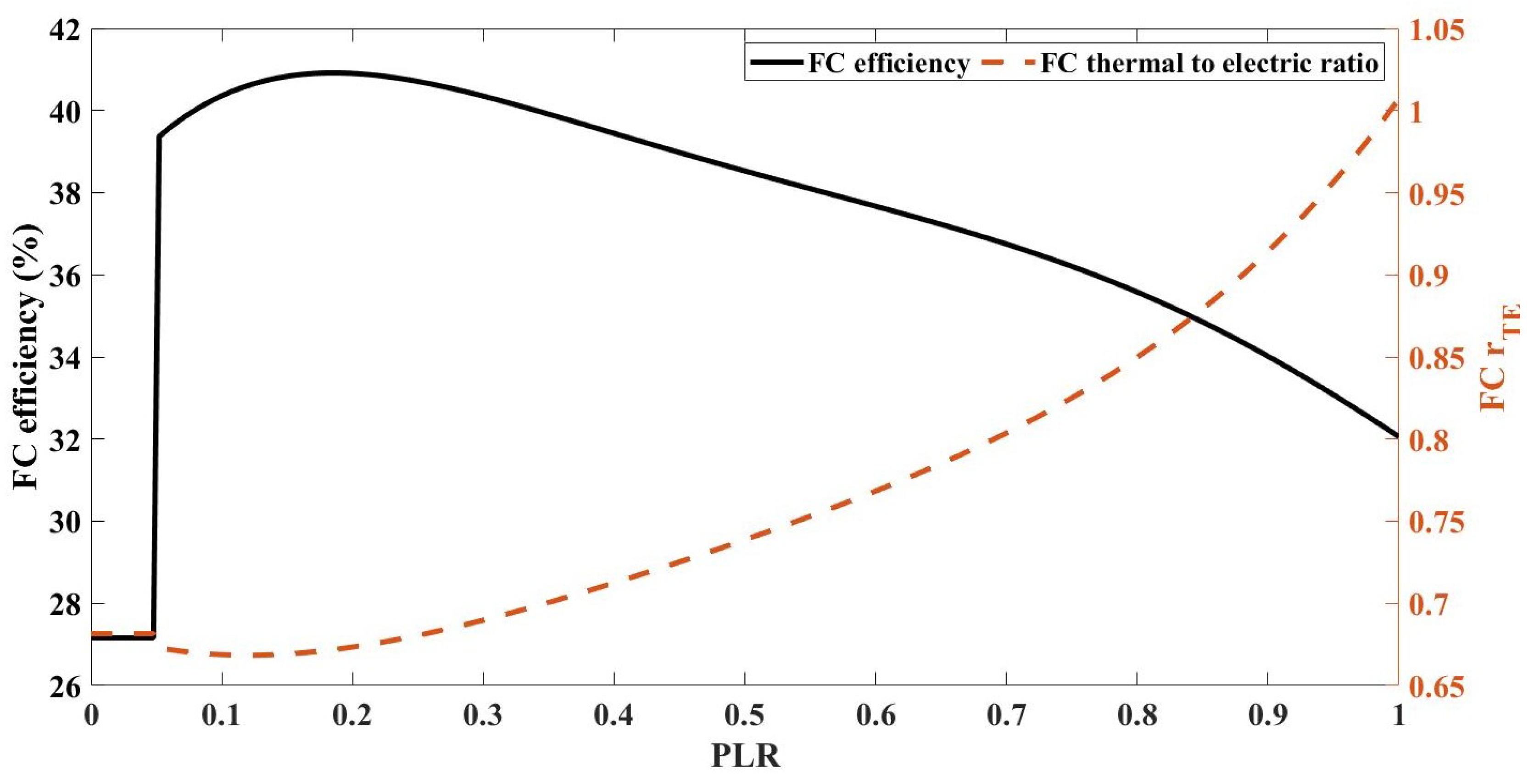
2.1. Modeling the FC

FCs have various types depending on their fuel types and construction. Figure 2 shows the main components of a typical FC. It consists of a fuel processing unit, a stack, and a power conditioning unit. A proton exchange membrane FC is used in this work whose input is natural gas and outputs are electrical power and heat.
The efficiency of an FC depends on its part load ratio (PLR). The PLR is the ratio of electrical power generated by the FC at the i-th interval to its power capacity rating as given in Equation (1):
P L R i = P F C . i / P F C m a x
where P L R i is the PLR at i-th interval for P F C . i output in this interval.
Mathematically, FC’s efficiency η F C and its thermal to electrical power ratio ( r T E . i ) are represented for the i-th interval as follows:
When P L R i < 0.05 :
η F C . i = 0.2716
r T E . i = 0.6816
When P L R i > 0.05 :
η F C . i = 0.9033 P L R i 5 2.9996 P L R i 4 + 3.6503 P L R i 3 2.0704 P L R i 2 + 0.4623 P L R i + 0.3747
r T E . i = 1.0785 P L R i 4 1.9739 P L R i 3 + 1.5005 P L R i 2 0.2817 P L R i + 0.6838
Next, the thermal power ( H F C . i ) generated by the FC at interval i is determined as:
H F C . i = r T E . i P F C . i
Figure 3 shows the relationship between PLR and the efficiency of FC. At low PLR (<5%), the efficiency of FC is low due to high parasitic losses [34]. Beyond this low PLR region, the FC works at 30–40% efficiency. Looking at the efficiency curve, it is evident that η F C is comparatively higher at lower PLR regions in contrast to the regions of FC’s peak power operation.

2.2. Modeling the EV

The model of an EV depends on various factors such as EV driving style, distance traveled, type of route, and SOC at plugged-out time. This work models the EV initial SOC at plugged-in time depending upon the daily traveled distance [31] and uses the data available in [35,36].
S O C E V . p i = S O C E V m i n i f S O C E V p o d η E V E V c a p S O C E V m i n S O C E V p o d η E V C E V O t h e r w i s e
where
P E V i , S O C E V . i Charging power (kW), and resultant SOC of EV (%) at interval i
S O C E V p i , S O C E V p o , S O C E V m i n Plugged-in, Plugged-out, and Minimum SOC of EV(%)
d,ηEVDaily traveled distance (km) and, Net drive efficiency (km/kWh) of EV
CEVEV battery capacity (kWh)
If d and S O C E V p o are known, then S O C E V p i is computed using Equation (7). It is evident from this equation that a lower boundary condition is applied to S O C E V p i to safeguard the EV batteries.
Equation (8) governs the EV charging process:
S O C E V . i = S O C E V . i 1 + P E V . i C E V × T × 100

2.3. Modeling the BESS

The charging and discharging of the BESS is governed by Equation (9).
W B . i = W B . i 1 + T η B . c h T η B . d c h μ i
where W B . i is the BESS energy at i-th interval, μ i = P B . i , c h P B . i , d c h is a column vector that contains charging and discharging powers of the BESS while η B . c h and η B . d c h are the respective charging and discharging efficiencies. T is the step time for simulation. P B . i , c h is the positive (+ve) value of P B . i and P B . i , d c h is the negative value of P B . i whenever it occurs. It should be noted that at any time interval only one value will exist in the μ i vector and the other value will be zero.

2.4. Electricity Import and Export Tariffs

A variable time-of-use tariff offers different electricity prices at different hours of the day to reduce the stress on electrical network and to improve the load factor of the power grid. In this work, a variable tariff known as ’peak-valley tariff’ is deployed for both import (buying) and export (selling) of the electrical energy [37,38]. This tariff has three rates (i.e., peak, plain, and valley) for different time slots of the day as explained in Table 1. Comparing the buying ( T b ) and selling ( T s ) tariffs in Table 1, it is evident that the values of both tariffs are different for their respective time intervals. The value of T s is actually less than T b to incentivize the buyer (in this case utility) to purchase electricity from the SH. The values of T b and T s are normalized with respect to the peak tariff and are used in Equation (13).

3. Optimization Model

The main purpose of an EMS is to optimize the power generation and use of different sources and loads to minimize the total cost while satisfying the load and devices constraints. This operating schedule of devices is performed one day ahead to ensure their effective use. The current section proposes an IHEMS for the SH optimization model. The 24-hour operational cost minimization of the SH is the ultimate objective of this paper subject to the following assumptions:
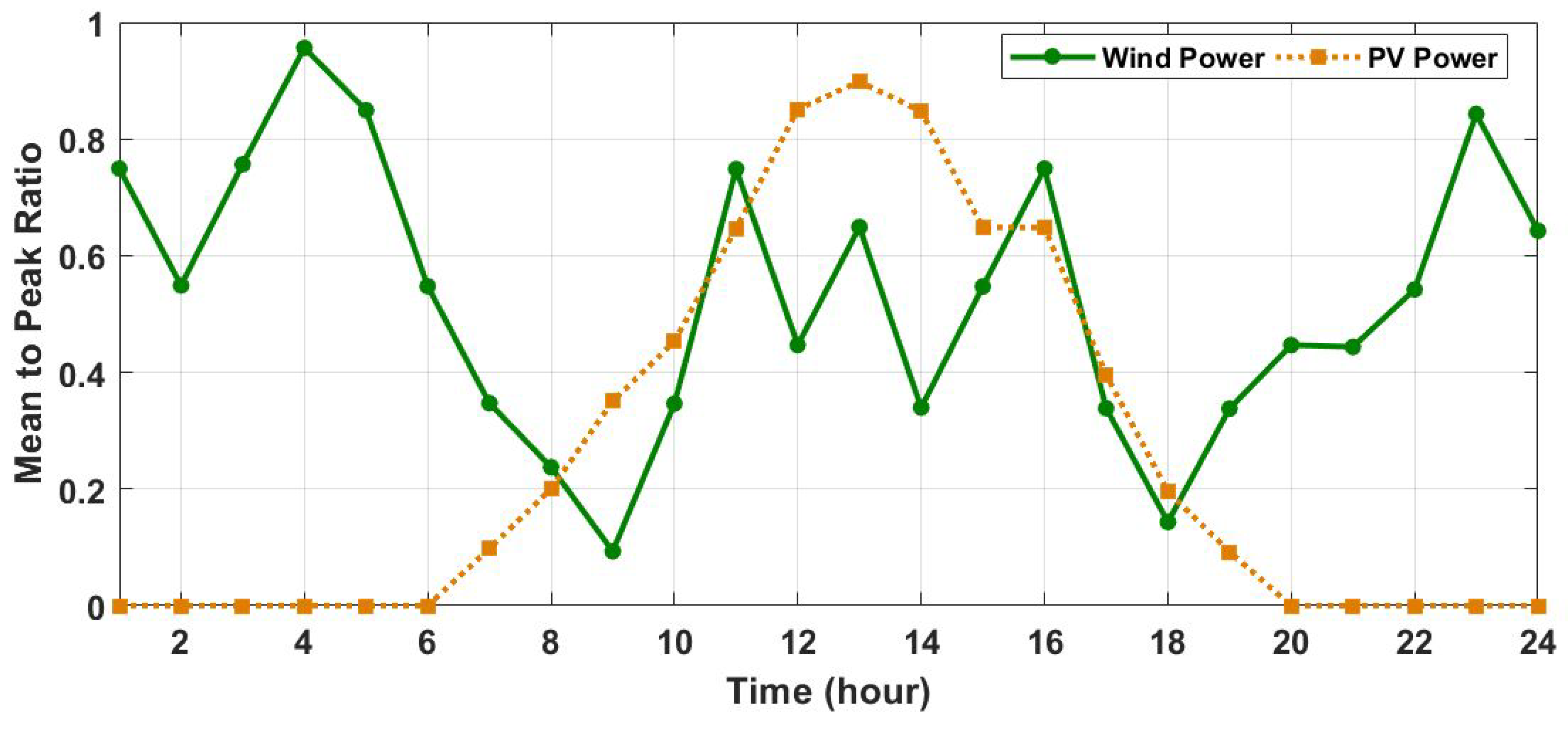
  • The forecasted data for wind and PV, and the thermal and electrical loads is available.
  • The EV daily trip distance as well as the initial energy levels of the BESS, are known.
  • The system installation costs are neglected.

3.1. Objective Function

The objective function is to minimize the total operating cost of the SH for 24-hours, as expressed in (10).
min i = 1 n C F C . i + C B L . i + C U . i + C B . i
C F C . i = T · C g a s P F C . i η F C . i + α if P F C . i 1 = 0 , and P F C . i > 0 β if P F C . i 1 > 0 , and P F C . i = 0 T · C g a s P F C . i η F C . i e l s e
C B L . i = T · C g a s · H B L . i
C U . i = T · T b · C U b · P U . i if P U . i 0 T · T s · C U s · P U . i if P U . i < 0
C B . i = C B o m · P B . i · T if P B . i 0 C B o m · P B . i · T if P B . i < 0
where
n,TTotal time, Span of the time interval (h)
α,βFC Startup, Shutdown costs ( $ )
CFC.i, CBL.i, CU.i, CB.iTotal cost of the FC, Boiler, Utility, BESS at interval i ( $ )
CgasCost for purchasing natural gas ( $ /kW)
CUb, CUbBase cost for Buying, Selling utility electricity ( $ /kW)
CBomOperation and maintenance cost of BESS ( $ /kW)
PFC.iFC electrical power output at interval i (kW)
HBL.iThermal power produced by the boiler at interval i (kW)
PU.iElectrical power purchased from, or sold to, the utility at interval i (kW).
Tb,TsMultipliers for Buying, Selling tariff as described in Table 1
ηFC.iFC efficiency
It should be noted that P U . i will be positive for purchasing and negative for selling electrical power to the utility.

3.2. Constraints

The devices installed and power requirements in the SH have certain mechanical and electrical operating limits. Therefore, constraints related to power balance and devices are defined in the following subsections.

3.2.1. Power Balance Constraints

Electrical Power Balance

If load shedding is to be avoided, the system should meet the electrical demand completely.
When BESS is charging, the electrical power balance should be:
P D . i + P E V . i P F C . i P W . i P P V . i P B . i η c h P U . i = 0
and in the discharging interval of the BESS, the electrical power balance should be:
P D . i + P E V . i P F C . i P W . i P P V . i η d c h P B . i P U . i = 0
where
PD.iElectrical demand at interval i (kW)
PW.i, PPV.iWind, PV powers at i-th interval (kW)
PB.iBESS charging or discharging power at i-th interval (kW).
PEV.iEV charging power at i-th interval (kW)
ηchdchCharging, Discharging efficiencies of the BESS ( p . u )
Here P B . i is negative in the charging interval of BESS and positive otherwise.

Thermal Power Balance

The thermal power is provided by FC and auxiliary boiler, therefore, following constraint must be satisfied to balance the thermal power requirements of the SH.
H D . i H F C . i H B L . i = 0
where H F C . i is the heating produced by FC (kW) and H B L . i is the auxiliary boiler output (kW) at interval i. H D . i is the thermal demand of the SH.

3.2.2. Constraints of Devices

The constraints applying to the devices in the SH are given as below.

Constraints of FC

For the smooth operation of the FC, the rate of change in its output power is subjected to ramp rate constrains.
P F C . i P F C . i 1 < Δ P F C u p
P F C . i 1 P F C . i < Δ P F C d n
Similarly, FC output is also bound by the minimum and maximum limits of power generation.
P F C m i n < P F C . i < P F C m a x
where
ΔPFCup, ΔPFCdnFC ramp up, ramp down rates
PFCmin, PFCmaxFC minimum, maximum power limit

Constraints of EV

The following EV charging and SOC limit must be taken into account to prevent damage to the EV battery.
P E V . i < P E V c h m a x
S O C E V m i n S O C E V . i S O C E V m a x
where P E V c h m a x is the upper limit of EV charging power in (kW) and S O C E V m a x denotes the maximum possible SOC of the EV battery.

Constraints of BESS

The following constraints for minimum and maximum energy of the BESS must be fulfilled.
W B m i n < W B . i < W B m a x
Depending on whether the BESS is charging or discharging, the rate of change of energy in the BESS in succeeding hours is limited by the maximum charging and discharging rates of the BESS power.
During charging interval:
W B . i W B . i 1 < P B c h m a x × T
During discharging interval:
W B . i 1 W B . i < P B d c h m a x × T
where
WB.iEnergy level in the BESS at i-th interval (kWh)
WBmin, WBmaxMinimum, Maximum energy limits in BESS (kWh)
PBchmax, PBdchmaxMaximum rates of Charging, Discharging of BESS (kW)

3.3. Renewable Energy Generation

The powers from wind and PV systems depend on the weather. Figure 4 shows a typical power curve of wind and PV [39]. During the daytime (10:00–17:00), wind power fluctuates sharply, while PV generates at its peak. PV stops working during the night because of the unavailability of the irradiance from the sun, while wind power generates its peak output energy. These two curves are used as estimated (forecasted) curves for wind and PV power in this model and mean to peak ratios of the values in these curves are 53.16%, 26.46% respectively.
Figure 5 presents the IHEMS. Its left section shows three main parts: forecast, optimization, and online control. The forecast model uses external forecasting data and foretells the generations from PV and wind, and predicts the electrical and thermal demands. The optimization model uses these predicted values and produces the optimized schedule for these devices to minimize the operational costs. The control model gets input from the online measurements, and balances the generation and load because of the inherent difference between the forecasted data and the actual requirement.
However, the forecasting of loads and renewable energy resources is a complex task. The data obtained from the forecast has a direct influence on the scheduling of system devices performed in the optimization model. The prediction modeling of renewable power generation has been a hot issue and it requires numerous factors to be considered. Researchers have developed a variety of prediction models. A wind-prediction framework based on chaotic time series and singular spectrum analysis is presented in [40]. Barque et al. presented the use of retraining machine learning algorithms to improve wind power prediction [41]. Results suggest a 17% increase in the prediction accuracy compared to persistence approach. A hybrid model for renewable energy and load prediction based on data mining is proposed in [42]. The outputs of these models (and others like them) enable us to use the optimization model to work out the power generations of energy resources for the forthcoming day. The main focus of this paper is to develop the optimization model for the SH. Therefore, it neglects the prediction and control models.
The right section of Figure 5 presents the flowchart for the RCGA-based optimal scheduling process. The details of these modules are presented in the next section.

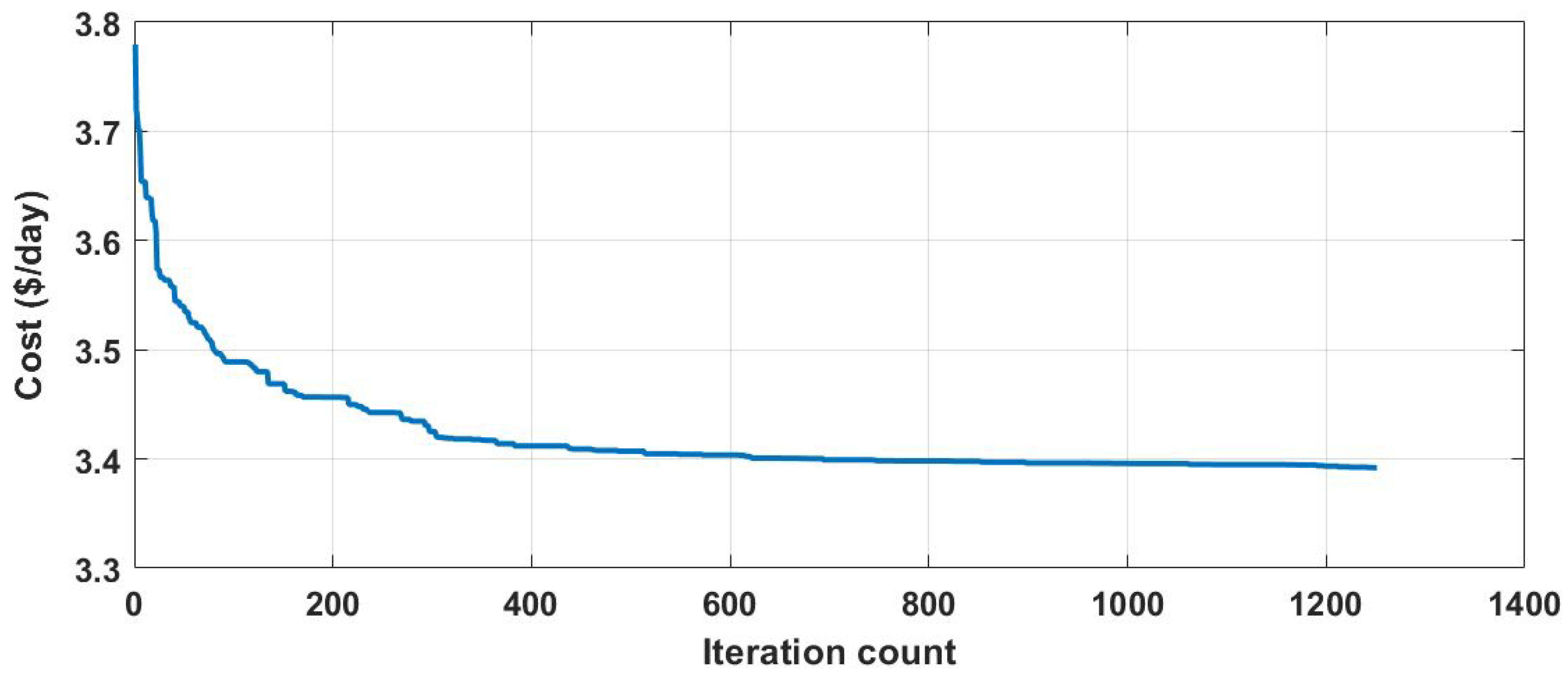
4. Real Coded Genetic Algorithm

The optimization models based on modern heuristics show better results in comparison to the conventional derivative-based models. Based on evolution in nature, Genetic Algorithm (GA) is one of the most popular algorithms used in power system applications. RCGA is an improved version of the GA which yields comparatively better results for real-valued numerical optimization problems. In RCGA, the population variables are represented by floating point or integer values in contrast to the GA which represents them as binary variables. Studies show that the RCGA generally result in faster convergence, more consistency, and higher precision in comparison to the GA [43,44,45,46]. This work uses RCGA to model and solve the optimization problem of IHEMS, and a summary of the steps involved in this process is presented in the following sections:

4.1. Step I: Initialization

Like other global optimization techniques, the first step in RCGA is to generate the initial population. This initial population is called chromosomes. The chromosomes are composed of genes where each gene represents power (kW) of a certain device installed in the SH. If N is the total number of genes in a chromosome, then the position of i-th gene is represented as:
C h r o m o s o m e i = x 1 , x 2 , x 3 , , x i , x N i = 1 , 2 , , N
It is important to take into account the dimensionality of the IHEMS. The system presented in this work is constitutes of dependent and independent variables. The independent variables are used by the RCGA for optimization. Here P F C , P E V , and P B are the independent variables. With their use, and with the use of fixed variables of power demands and renewable resources, the remaining dependent variables of H F C , P U , H B L , P L R , η F C , r T E etc. are computed. Finally, these variables are used in Equations (11)–(16) to calculate the cost.
The RCGA calculates the cost of the SH for a 24 h period. The time interval used in this study is 1 h. Therefore, the IHEMS is studied for 24 time sections with 3 variables ( P F C , P E V , P B ) in each interval resulting in the size of optimization problem N = 24 × 3 = 72 .
Expression below represents one chromosome of the RCGA with each power denoting one gene of the chromosome.
P E V 1 1 P E V 1 2 P E V 1 24 P F C 1 1 P F C 1 2 P F C 1 24 P B 1 1 P B 2 P B 1 24

4.2. Step 2: Implementation of the Constraints

The system constraints for P F C . i , H B L . i and P E V . i are checked during each time interval. The equations governing this step are given in Section 3.2.2. The logical process and variable operations in the RCGA for the fulfillment of these constraints are given in the flow chart in Figure 5.

4.3. Step 3: Using RCGA Operators

4.3.1. Selection

The selection of the fittest individual to the successive generation is a significant process in the RCGA. The individuals (chromosomes) are carefully chosen for the succeeding generations based on their fitness value. Ranking, tournament, and roulette-wheel are some commonly used selection strategies. In this work, the selection procedure is carried out by the roulette-wheel selection method [47].

4.3.2. Crossover

For the RCGA to be able to successfully search the promising solution, the search space must be reachable by the initial population. To ensure this global search property of the GA, a crossover operation is used. This operator performs a crucial role in RCGAs. In reality, it is regarded as its defining characteristic [48]. It should be observed that during the process of generating intermediate populations, all chromosomes are not subject to this operator. An arbitrary choice is made, where the chance of crossover application on a chromosome pair is determined by the crossover rate also known as the crossover probability, P c [49].

4.3.3. Mutation

The mutation operator randomly modifies one or more genes of a certain chromosome to enhance the fundamental variability of the population. Without mutation RCGA can prematurely converge to sub-optimal solutions. The role of this operator is to reinstate the unexplored or lost; but possible solutions into search space of the population. Mutation ensures a non-zero probability of the RCGA algorithm to arrive at any solution in the search space. All positions of each chromosome in the population has an arbitrary chance of undergoing into a random alteration. This alteration chance is defined by a mutation rate, or mutation probability, P m . Muhlenbeins Mutation operator described in [50] is used in this work.
With crossover and mutation, another selection approach, called elitism is also adopted to make certain that the best performing chromosomes always survive unharmed from the previous to the subsequent generations [51].

5. Simulation Results

This section presents multiple simulation scenarios to demonstrate the important features of the proposed optimization model. The RES, FC, BESS, variable tariff and EV are added incrementally into the IHEMS as summarized in Table 2. In all the cases, the electric power can be purchased from and sold to the utility and the auxiliary boiler is available for thermal power requirements.
Figure 6 shows the normalized electrical and thermal load requirements of a typical SH [52]. The peak electricity and thermal demands are 1.8 kW and 2 kW, respectively for the SH. For the EV, a Mitsubishi’s compact i-MiEV is used in this work [53]. The U.S. National Household Travel Survey (NHTS) is used to select EV parameters of T i , T o and d [35,36]. The numerical values of the parameters used in this study are summarized in Table 3.

5.1. Base Case

In this mode of operation, electrical load is powered by the utility and the thermal load is supplied by the gas boiler. No other devices are available in this case as shown in Table 2. The operating cost of the house in this case is $6.84 per day, and it will be used as a reference for later cases.

5.2. Case 1: Addition of RES

In this mode of operation, a solar and wind-based RES is installed in the SH with the following considerations:
  • In supplying the electrical loads, the wind and solar power resources must be given priority.
  • Heating is still provided by the auxiliary boiler.
  • Bidirectional power flow is considered. In this way, the consumers can sell surplus electric energy to the utility.
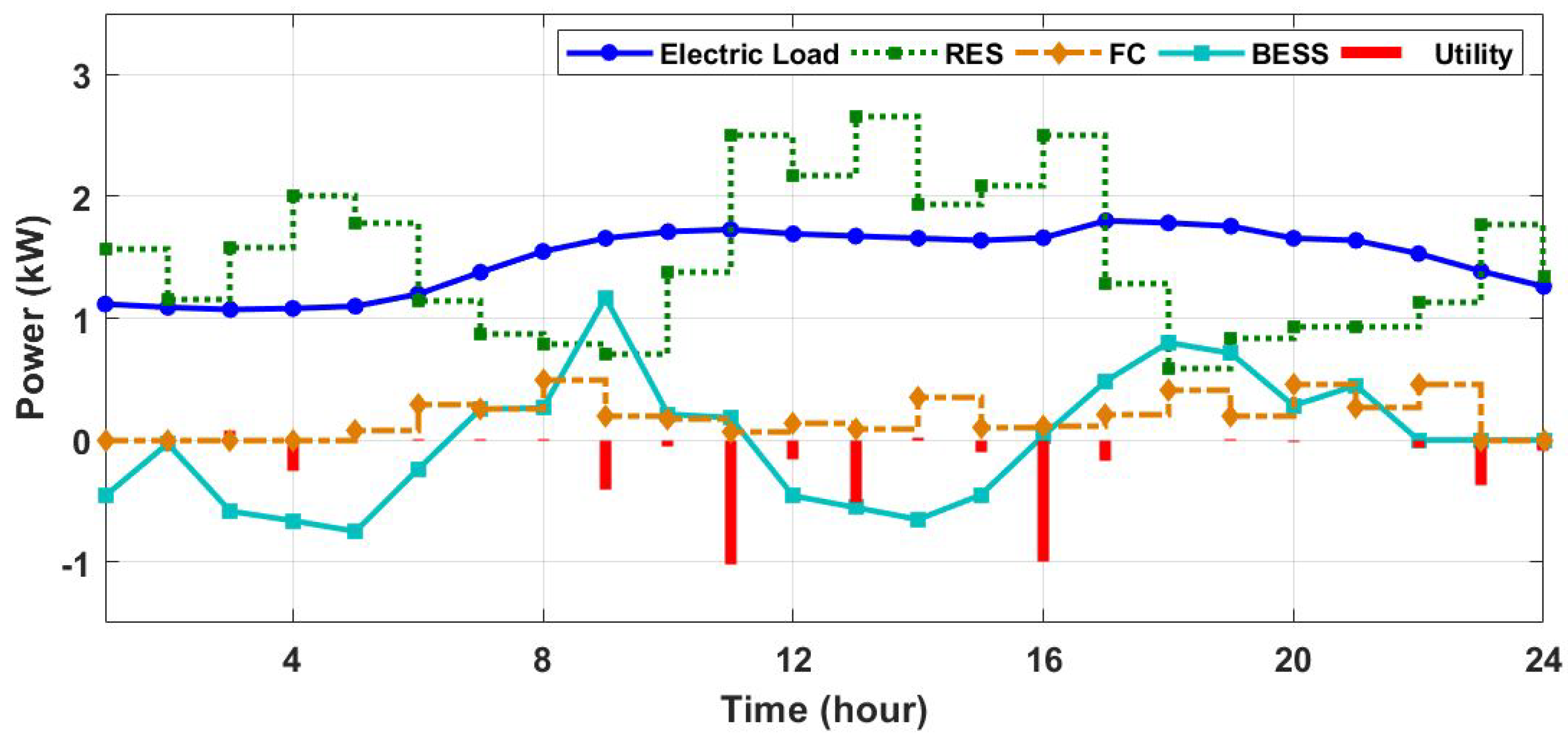
  • The RES curve in the subsequent figures is the summation of both wind and PV output powers in each time interval.
Figure 7 shows the optimal allocation of HES where the negative utility powers indicate the utility power purchase from the SH. In the intervals 01:00–05:00, 11:00–16:00 and 23:00–24:00 the electrical load is less than the total RES generation, and the SH is selling excessive energy to the utility. The peak loading in the system occurs in 06:00–10:00 and 17:00–22:00 when the RES cannot fulfill the demand, therefore, the power is purchased from the utility. The daily operational expenses of the SH are $2.6272 in this case.

5.3. Case 2: FC Included

In this case, the FC-based micro-CHP system is included in the IHEMS. Thermal output of the FC and the boiler satisfy the thermal load demand, while the RES and electrical output of the FC supply the electrical load of the house in combination with the utility.
As shown in Figure 8, the FC is idle in the early hours of the day. At 6:00 A.M., when the load demand exceeds the RES power, the FC starts its operation to meet the load demand. Most of the time, no power is purchased from the utility in this mode while selling the surplus power during 01:00–05:00, 11:00–16:00 and 23:00–24:00 time intervals. However, at 18:00 the combined output of the FC and the RES is unable to meet the load demand. Therefore, electric power is purchased from the utility during this hour.
An important observation in this case is the low power operation of the FC during 11:00–16:00. The reason behind this behavior of the FC is the consideration of startup and shutdown costs of the FC in the developed model. The inherent nature of the RCGA is to move towards an optimal cost; therefore, the algorithm calculates and compares if it is beneficial to shut down the FC or to keep it operating at a lowest optimum level. During this time period, the FC is running at its minimum possible output described as P F C m i n . The daily operational cost of the SH is $2.3968 in this case which is a decrease of 8% as compared to Case 1.

5.4. Case 3: BESS Included

In this case, a BESS is added to the SH which can store the surplus power available in the SH. Figure 9 shows the optimal hourly allocation of the BESS proposed by the IHEMS. A detailed explanation of BESS charging and discharging and its energy routing dependence upon the efficiency has already been presented in [33] by the same authors. The operational cost of the SH is $2.337 in this case which is a reduction of 3% compared to case 2.

5.5. Case 4: Variable Tariff Considered

In this case, a peak-valley tariff is considered for the purchase and sale of electricity as given in Table 1. The hourly allocation of the HES is similar to what was observed in Case 3. However, total cost in this case is $2.30 which is a drop of 2% in comparison to the cost in case 3. This difference is comparatively small although a substantial cost saving was anticipated because of peak-valley tariff. This is due to the fact that price for selling the excessive electricity has reduced too in intermediate and valley periods of the tariff to incentivize the buyer.
Case 5 and 6 evaluate the impacts of EV charging on the utility loading and the SH’s daily energy cost. The study of EV charging is divided into two cases: Case 5 considers the EV charging without any scheduling, and Case 6 has three charging strategies which consider the schedulable EV charging. Table 4 summarizes the characteristics of four electric vehicle supply equipment (EVSE) for EV charging. The impact of these charging techniques on charging powers of EV and utility loading are presented in Figures 11 and 12.

5.6. Case 5: EV Included

In this case, an EV is added to the SH which is charged by a charging strategy named as EVSE-1. The EV charges with a constant rate of maximum charging capability of the charger which is 3.3 kW. It presents itself as a constant load from the time it is plugged-in ( T I ) until it gets fully charged as shown in Figure 10. A comparative view of this charging technique with others EVSEs is depicted in Figure 11. This is the simplest charging strategy, termed as “dumb charging”.
In this case, the cost has increased to $3.58 due to power demand by the EV. This type of charging method exerts a significant loading on the utility. The maximum utility loading in this case is 3.02 kW at 20:00 as shown in Figure 12.

5.7. Case 6: Scheduling of the EV Charging

In this case, EV is modeled as a schedulable load and gets scheduled considering it a responsive demand. An EVSE type is selected from Table 4 from EVSE 2 to 4. Under this case, the EV is scheduled and charged in such a way that the overall cost of powering the SH decreases. The demand response algorithm shifts the EV charging considering multiple factors. These factors are prioritized according to the cost of power. The first priority is the availability of power from the RES. The EV gets charged in those hours when RES generation is available after fulfilling critical load demand. The second priority is to shift the EV charging to the hours of valley tariff. The proposed IHEMS schedules the charging of the EV using various EVSEs as explained in the following subsections:

5.7.1. EVSE-2

In this charging strategy, the EV is charged with the same charger as that of EVSE-1 with an added capability of turning on and off at a particular hour as commanded by the IHEMS. This mode shifts the charging of the EV on the time axis as shown in Figure 11. The charging time is shifted depending upon the utility tariff or status of HES.
Figure 11 shows that the charging time is shifted from ( T I ) to the low utility tariff window (i.e., 23:00 to 08:00). The EV is charged from 22:00 to 23:00 and then charging is stopped from 23:00 to 02:00 due of the unavailability of surplus power from the RES. Although the RES power is not zero from 23:00 to 02:00, it must meet the demand of critical loads (please refer to Figure 7 for the RES generation and load demand curves). The charging starts again at 03:00 when surplus wind energy is available.
In this mode of charging, the peak utility loading occurs at 23:00, but this peak is less than the peak observed for EVSE-1 in Case 5. The maximum utility loading of 2.49 kW is noted in this case which is a 17.6% reduction compared to EVSE-1 as shown in Figure 12. The energy cost is $3.30 which is an 8% reduction in comparison to EVSE-1.

5.7.2. EVSE-3

This charging strategy implements a variable charger with discrete charging powers. An example is the Siemens VersiCharge systems [54]. This work considers the discrete power values of {3.3, 3, 2.7, 2.4, 2.1} kW, and the charger can turn on and off according to the signals from the IHEMS. Figure 11 shows that EV charging has expanded to 5 h as compared to EVSE-1 and EVSE-2. This charging strategy enables the EV to get charged more from the RES, and consequently, the utility loading decreases as shown in Figure 12. The peak utility load decreases to 1.14 kW at 01:00, which is a 62% decrease as compared to EVSE-1.

5.7.3. EVSE-4

This charging strategy considers an adaptive charger and EV gets charged rigorously according to the continuous values of power given by the IHEMS. Intuitively, the algorithm tries to follow the RES power availability trend to charge the EV as shown in Figure 11. The RES power is used at its maximum level, and the utility loading decreases further to 0.31 kW at 05:00 as shown in Figure 12. This is a decrease of 90% compared to EVSE-1. The reason for this large reduction in utility loading is the adaptive nature of EVSE-4 that resulted in the EV charging time expansion to 14 h in search for the surplus power from the RES. The cost of 24-hours operation of the SH decreases to $3.24 which is 9.5% less than the cost for EVSE-1. Figure 13 presents the electrical powers of each device installed in the SH, and Figure 14 shows the thermal powers from the FC and boiler for this case.
The cost comparison between EVSE-1 and EVSE-2 shows a cost reduction of 8% although EVSEs for the two cases have the same constant charging powers. This difference is due to considering the EV as a schedulable load. The impact of different chargers on cost is minimal as the difference between EVSE-4 and EVSE-2 is only 1.5%. However, in comparison to EVSE-1, the peak load on the utility decreases by 17.6%, 62% and 90% by using EVSE-2, EVSE-3, and EVSE-4, respectively. Therefore, the scheduling of the EV is beneficial for the power system operator as it reduces the urgent need for generation capacity enhancement and expansion of transmission and distribution networks. This is the case in many places around the world. Toronto, Canada [55] and Perth, Western Australia [56], are the examples of two places where this is a big concern and researchers advised using the controlled charging schemes for reducing the loading impacts of the EVs.
A summary of the costs of the boiler, the FC and the utility is presented in Table 5 for each case. Savings in the net cost relative to the previous and the base case is also presented at the end of this table. A negative utility cost shows a net profit to the SH for 24 h. A negative saving value relative to the previous case represents an increase in the SH operating cost as shown by −55 % for case 5.
Figure 15 shows the convergence of RCGA for Case 6. It is evident that the algorithm moves rapidly towards the optimal solution in the initial generations, and takes around 600 generations to converge at the optimal cost.
Table 6 provides the numerical values of the power demands and generations, and the costs for the 24-hours operation of the SH. The costs for the FC, boiler, and utility make a major part of the total cost of the SH. The total cost for the operation and maintenance of the BESS is very small (i.e., $0.0062 per day), and is not shown in the cost table. This table can serve as a look up table for the comparison purpose by the future researchers if they work on similar simulation conditions.

6. Conclusions

The present climatic and economic circumstances of the world necessitate an increased role of HES and EVs at domestic levels, and a significant research work is devoted to effectively accommodate their role. Adding to the existing literature, this work defined and modeled an IHEMS in the framework of modern SHs to optimize their economic operation using RCGA. To meet the thermal and electrical demands, the developed SH model included a HES which (in an all-inclusive case) consisted of natural gas-based micro-CHP system and electric power from a utility, a BESS, a wind turbine, and a PV system. In this study, a modern utility grid which allows a bidirectional power flow was considered where the customer can sell their surplus energy to the utility. Keeping in view the high loading impacts of the EV, typical EV charging methods were incorporated, and their impact on the SH’s economy was discussed. The developed IHEMS optimally scheduled the energy resources and EV charging simultaneously, and resulted in a cost-effective economic operation of the SH as indicated by the simulation results. A comparison of costs and savings of SH devices was summarized to show the features of the developed model. Moreover, a comparison of different EVSEs showed that flexible charging mechanism was beneficial for both the customer and the utility. The work revealed that optimal use of HES improved the economy of SHs while reducing the utility loading in the presence of EVs. This work may be extended in future to include stochastic behavior of various components of SH. Similarly considering thermal energy storage devices and a bidirectional flow of thermal energy in the proposed model may yield interesting results.

Author Contributions

Conceptualization, M.K.R.; Resources, S.U.K., S.B.A.B. and C.-H.K.; Software, K.K.M. and Z.M.H.; Writing—original draft, M.K.R. and M.S.U.Z.; Writing— review & editing, M.K.R., S.U.K. and M.S.U.Z.

Funding

This research was funded by "National Research Foundation of Korea(NRF) grant funded by the Korea government(MSIP), grant number 2018R1A2A1A05078680” and “The APC was funded by the authors”.

Conflicts of Interest

The authors declare no conflict of interest.

References

  1. Rolfsman, B. CO2 emission consequences of energy measures in buildings. Build. Environ. 2002, 1421–1430. [Google Scholar] [CrossRef]
  2. Murugan, S.; Horák, B. A review of micro combined heat and power systems for residential applications. Renew. Sustain. Energy Rev. 2016, 64, 144–162. [Google Scholar] [CrossRef]
  3. Benam, M.R.; Madani, S.S.; Alavi, S.M.; Ehsan, M. Optimal Configuration of the CHP System Using Stochastic Programming. IEEE Trans. Power Deliv. 2015, 30, 1048–1056. [Google Scholar] [CrossRef]
  4. El-Sharkh, M.Y.; Rahman, A.; Alam, M.S.; El-Keib, A.A. Thermal energy management of a CHP hybrid of wind and a grid-parallel PEM fuel cell power plant. In Proceedings of the 2009 IEEE/PES Power Systems Conference and Exposition, Seattle, WA, USA, 15–18 March 2009; pp. 1–6. [Google Scholar]
  5. Nehrir, M.H.; Wang, C. Hybrid Fuel Cell Based Energy System Case Studies. In Modeling and Control of Fuel Cells: Distributed Generation Applications; Wiley-IEEE Press: Hoboken, NJ, USA, 2009; pp. 219–264. [Google Scholar] [CrossRef]
  6. Adam, A.; Fraga, E.S.; Brett, D.J.L. Options for residential building services design using fuel cell based micro-CHP and the potential for heat integration. Appl. Energy 2015, 138, 685–694. [Google Scholar] [CrossRef]
  7. Feng, Z.B.; Jin, H.G. Part-load performance of CCHP with gas turbine and storage system. Proc. CSEE 2006, 26, 25–30. [Google Scholar]
  8. Combined Heat and Power (CHP). Available online: http://aceee.org/topics/combined-heat-and-power-chp (accessed on 25 February 2019).
  9. Khan, S.U.; Mehmood, K.K.; Haider, Z.M.; Rafique, M.K.; Kim, C.H. A Bi-Level EV Aggregator Coordination Scheme for Load Variance Minimization with Renewable Energy Penetration Adaptability. Energies 2018, 11, 2809. [Google Scholar] [CrossRef]
  10. Khan, S.U.; Mehmood, K.K.; Haider, Z.M.; Bukhari, S.B.A.; Lee, S.J.; Rafique, M.K.; Kim, C.H. Energy Management Scheme for an EV Smart Charger V2G/G2V Application with an EV Power Allocation Technique and Voltage Regulation. Appl. Sci. 2018, 8, 648. [Google Scholar] [CrossRef]
  11. García-Villalobos, J.; Zamora, I.; San Martín, J.I.; Asensio, F.J.; Aperribay, V. Plug-in electric vehicles in electric distribution networks: A review of smart charging approaches. Renew. Sustain. Energy Rev. 2014, 38, 717–731. [Google Scholar] [CrossRef]
  12. Sanguinetti, A.; Karlin, B.; Ford, R.; Salmon, K.; Dombrovski, K. What’s energy management got to do with it? Exploring the role of energy management in the smart home adoption process. Energy Effic. 2018, 11, 1897–1911. [Google Scholar] [CrossRef]
  13. Ford, R.; Pritoni, M.; Sanguinetti, A.; Karlin, B. Categories and functionality of smart home technology for energy management. Build. Environ. 2017, 123, 543–554. [Google Scholar] [CrossRef]
  14. Xie, D.; Lu, Y.; Sun, J.; Gu, C.; Li, G. Optimal Operation of a Combined Heat and Power System Considering Real-time Energy Prices. IEEE Access 2016, 4, 3005–3015. [Google Scholar] [CrossRef]
  15. Ashique, R.H.; Salam, Z.; Aziz, M.J.B.A.; Bhatti, A.R. Integrated photovoltaic-grid dc fast charging system for electric vehicle: A review of the architecture and control. Renew. Sustain. Energy Rev. 2017, 69, 1243–1257. [Google Scholar] [CrossRef]
  16. Dubey, A.; Santoso, S. Electric Vehicle Charging on Residential Distribution Systems: Impacts and Mitigations. IEEE Access 2015, 3, 1871–1893. [Google Scholar] [CrossRef]
  17. Cao, Y.; Tang, S.; Li, C.; Zhang, P.; Tan, Y.; Zhang, Z.; Li, J. An Optimized EV Charging Model Considering TOU Price and SOC Curve. IEEE Trans. Smart Grid 2012, 3, 388–393. [Google Scholar] [CrossRef] [Green Version]
  18. Romano, R.; Siano, P.; Acone, M.; Loia, V. Combined Operation of Electrical Loads, Air Conditioning and Photovoltaic-Battery Systems in Smart Houses. Appl. Sci. 2017, 7, 525. [Google Scholar] [CrossRef]
  19. Mohsenian-Rad, H.; Ghamkhari, M. Optimal Charging of Electric Vehicles With Uncertain Departure Times: A Closed-Form Solution. IEEE Trans. Smart Grid 2015, 6, 940–942. [Google Scholar] [CrossRef]
  20. Saeed Uz Zaman, M.; Bukhari, S.B.A.; Hazazi, K.M.; Haider, Z.M.; Haider, R.; Kim, C.H. Frequency Response Analysis of a Single-Area Power System with a Modified LFC Model Considering Demand Response and Virtual Inertia. Energies 2018, 11, 787. [Google Scholar] [CrossRef]
  21. Haider, Z.M.; Mehmood, K.K.; Rafique, M.K.; Khan, S.U.; Soon-Jeong, L.; Chul-Hwan, K. Water-filling algorithm based approach for management of responsive residential loads. J. Mod. Power Syst. Clean Energy 2018, 6, 118–131. [Google Scholar] [CrossRef]
  22. Yao, L.; Damiran, Z.; Lim, W.H. Optimal Charging and Discharging Scheduling for Electric Vehicles in a Parking Station with Photovoltaic System and Energy Storage System. Energies 2017, 10, 550. [Google Scholar] [CrossRef]
  23. Angrisani, G.; Canelli, M.; Roselli, C.; Sasso, M. Integration between electric vehicle charging and micro-cogeneration system. Energy Convers. Manag. 2015, 98, 115–126. [Google Scholar] [CrossRef]
  24. Yokoyama, T.W.N.W.R. Energy-saving effect of a residential polymer electrolyte fuel cell cogeneration system combined with a plug-in hybrid electric vehicle. Energy Convers. Manag. 2014, 77, 40–51. [Google Scholar] [CrossRef]
  25. Yokoyama, T.W.N.W.R. Feasibility study on combined use of residential SOFC cogeneration system and plug-in hybrid electric vehicle from energy-saving viewpoint. Energy Convers. Manag. 2012, 170–179. [Google Scholar] [CrossRef]
  26. Entchev, H.R.E. Exploring the potential synergy between micro-cogeneration and electric vehicle charging. Appl. Therm. Eng. 2014, 677–685. [Google Scholar] [CrossRef]
  27. Liu, H.; Wang, B.; Wang, N.; Wu, Q.; Yang, Y.; Wei, H.; Li, C. Enabling strategies of electric vehicles for under frequency load shedding. Appl. Energy 2018, 228, 843–851. [Google Scholar] [CrossRef]
  28. Jin, C.; Sheng, X.; Ghosh, P. Energy efficient algorithms for Electric Vehicle charging with intermittent renewable energy sources. In Proceedings of the 2013 IEEE Power Energy Society General Meeting, Vancouver, BC, Canada, 21–25 July 2013; pp. 1–5. [Google Scholar] [CrossRef]
  29. Domínguez-Navarro, J.; Dufo-López, R.; Yusta-Loyo, J.; Artal-Sevil, J.; Bernal-Agustín, J. Design of an electric vehicle fast-charging station with integration of renewable energy and storage systems. Int. J. Electr. Power Energy Syst. 2019, 105, 46–58. [Google Scholar] [CrossRef]
  30. Choi, S.H.; Hussain, A.; Kim, H.M. Adaptive Robust Optimization-Based Optimal Operation of Microgrids Considering Uncertainties in Arrival and Departure Times of Electric Vehicles. Energies 2018, 11, 2646. [Google Scholar] [CrossRef]
  31. Wu, X.; Hu, X.; Yin, X.; Moura, S.J. Stochastic Optimal Energy Management of Smart Home With PEV Energy Storage. IEEE Trans. Smart Grid 2018, 9, 2065–2075. [Google Scholar] [CrossRef]
  32. Liu, Z.; Wu, Q.; Shahidehpour, M.; Li, C.; Huang, S.; Wei, W. Transactive Real-time Electric Vehicle Charging Management for Commercial Buildings with PV On-site Generation. IEEE Trans. Smart Grid 2018. [Google Scholar] [CrossRef]
  33. Rafique, M.K.; Haider, Z.M.; Mehmood, K.K.; Saeed Uz Zaman, M.; Irfan, M.; Khan, S.U.; Kim, C.H. Optimal Scheduling of Hybrid Energy Resources for a Smart Home. Energies 2018, 11, 3201. [Google Scholar] [CrossRef]
  34. Gunes, M.B. Investigation of a Fuel Cell Based Total Energy System for Residential Applications. Ph.D. Thesis, Virginia Tech, Blacksburg, VA, USA, 2001. [Google Scholar]
  35. Methipara, J.; Reuscher, T.; Santos, A. Electric Vehicle Feasibility: Can EVs Take US Households to Where They Need to Go? Technical Report; National Household Travel Survey: Washington, DC, USA, 2016.
  36. Santos, A.; McGuckin, N.; Nakamoto, H.Y.; Gray, D.; Liss, S. Summary of Travel Trends; Technical Report; National Household Travel Survey, Department of Transportation: Washington, DC, USA, 2009.
  37. Hu, Z.; Han, X.; Wen, Q. Integrated Resource Strategic Planning and Power Demand-Side Management; Power Systems; Springer: Berlin, Germany, 2013. [Google Scholar]
  38. Gianfreda, A.; Grossi, L. Zonal price analysis of the Italian wholesale electricity market. In Proceedings of the 2009 6th International Conference on the European Energy Market, Leuven, Belgium, 27–29 May 2009; pp. 1–6. [Google Scholar] [CrossRef]
  39. Gu, W.; Wu, Z.; Yuan, X. Microgrid economic optimal operation of the combined heat and power system with renewable energy. In Proceedings of the 2010 IEEE Power and Energy Society General Meeting, Minneapolis, MN, USA, 25–29 July 2010; pp. 1–6. [Google Scholar] [CrossRef]
  40. Safari, N.; Chung, C.Y.; Price, G.C.D. Novel Multi-Step Short-Term Wind Power Prediction Framework Based on Chaotic Time Series Analysis and Singular Spectrum Analysis. IEEE Trans. Power Syst. 2018, 33, 590–601. [Google Scholar] [CrossRef]
  41. Barque, M.; Martin, S.; Vianin, J.E.N.; Genoud, D.; Wannier, D. Improving wind power prediction with retraining machine learning algorithms. In Proceedings of the 2018 International Workshop on Big Data and Information Security (IWBIS), Jakarta, Indonesia, 12–13 May 2018; pp. 43–48. [Google Scholar] [CrossRef]
  42. Dou, C. Hybrid model for renewable energy and loads prediction based on data mining and variational mode decomposition. IET Gener. Transm. Distrib. 2018, 12, 2642–2649. [Google Scholar] [CrossRef]
  43. Michalewicz, Z. Genetic Algorithms + Data Structures = Evolution Programs, 3rd ed.; Springer-Verlag: London, UK, 1996. [Google Scholar]
  44. Damousis, I.G.; Bakirtzis, A.G.; Dokopoulos, P.S. Network-constrained economic dispatch using real-coded genetic algorithm. IEEE Trans. Power Syst. 2003, 18, 198–205. [Google Scholar] [CrossRef] [Green Version]
  45. Kuri-Morales, A.F.; Gutiérrez-García, J. Penalty Function Methods for Constrained Optimization with Genetic Algorithms: A Statistical Analysis. In Proceedings of the MICAI 2002: Advances in Artificial Intelligence: Second Mexican International Conference on Artificial Intelligence Mérida, Yucatán, Mexico, 22–26 April 2002; Coello Coello, C.A., de Albornoz, A., Sucar, L.E., Battistutti, O.C., Eds.; Springer: Berlin/Heidelberg, Germany, 2002; pp. 108–117. [Google Scholar] [CrossRef]
  46. Amjady, N.; Nasiri-Rad, H. Economic dispatch using an efficient real-coded genetic algorithm. IET Gener. Transm. Distrib. 2009, 3, 266–278. [Google Scholar] [CrossRef]
  47. Goldberg, D. Genetic Algorithms in Search, Optimization, and Machine Learning; Artificial Intelligence; Addison-Wesley Publishing Company: Boston, MA, USA, 1989. [Google Scholar]
  48. Blasco Ferragud, F.X. Control Predictivo Basado en Modelos Mediante Tecnicas de Optimizacion Heuristica. Aplicacion a Procesos no Lineales y Multivariables. Ph.D. Thesis, Universitat Politècnica de València, València, Spain, 1999. [Google Scholar]
  49. Herrera, F.; Lozano, M.; Verdegay, J. Tackling Real-Coded Genetic Algorithms: Operators and Tools for Behavioural Analysis. Artif. Intell. Rev. 1998, 12, 265–319. [Google Scholar] [CrossRef]
  50. Mühlenbein, H.; Schlierkamp-Voosen, D. Predictive Models for the Breeder Genetic Algorithm–I. Continuous Parameter Optimization. Evolut. Comput. 1993, 1, 25–49. [Google Scholar] [CrossRef]
  51. De Jong, K.A. An Analysis of the Behavior of a Class of Genetic Adaptive Systems. Ph.D. Thesis, University of Michigan, Ann Arbor, MI, USA, 1975. [Google Scholar]
  52. Linkevics, O.; Sauhats, A. Formulation of the objective function for economic dispatch optimisation of steam cycle CHP plants. In Proceedings of the 2005 IEEE Russia Power Tech, St. Petersburg, Russia, 27–30 June 2005; pp. 1–6. [Google Scholar] [CrossRef]
  53. Mitsubihsi i-MiEV Specifications. Available online: https://www.mitsubishi-motors.com/en/showroom/i-miev/specifications/ (accessed on 25 February 2019).
  54. Charging Unit VersiCharge IEC. Available online: https://www.siemens.com/global/en/home/products/energy/low-voltage/components/electric-vehicle–ev–charging/versicharge-iec.html (accessed on 25 February 2019).
  55. Awadallah, M.A.; Singh, B.N.; Venkatesh, B. Impact of EV Charger Load on Distribution Network Capacity: A Case Study in Toronto. Can. J. Electr. Comput. Eng. 2016, 39, 268–273. [Google Scholar] [CrossRef]
  56. McCarthy, D.; Wolfs, P. The HV system impacts of large scale electric vehicle deployments in a metropolitan area. In Proceedings of the 2010 20th Australasian Universities Power Engineering Conference, Christchurch, New Zealand, 5–8 December 2010; pp. 1–6. [Google Scholar]
Figure 1. A smart house overview.
Applsci 09 01658 g001
Figure 2. Typical Model of an FC.
Applsci 09 01658 g002
Figure 3. Representation of part load ratio’s role on efficiency and thermal to electrical ratio of FC.
Applsci 09 01658 g003
Figure 4. Wind and PV Power Curve.
Applsci 09 01658 g004
Figure 5. Flow chart of the proposed IHEMS with RCGA.
Applsci 09 01658 g005
Figure 6. Daily thermal and electric power demands.
Applsci 09 01658 g006
Figure 7. Installation of RES and Utility Bidirectional Power Flow.
Applsci 09 01658 g007
Figure 8. Hybrid energy supply with the FC.
Applsci 09 01658 g008
Figure 9. Optimized generation schedule with BESS included.
Applsci 09 01658 g009
Figure 10. Optimized generation schedule with EV included but unscheduled.
Applsci 09 01658 g010
Figure 11. EV charging powers for different EVSE.
Applsci 09 01658 g011
Figure 12. Power purchased from the utility with different EVSE.
Applsci 09 01658 g012
Figure 13. Optimized generation schedule with adaptive EVSE.
Applsci 09 01658 g013
Figure 14. Contribution of FC and the boiler to satisfy the thermal demand in system.
Applsci 09 01658 g014
Figure 15. Characteristics of RCGA convergence.
Applsci 09 01658 g015
Table 1. Electricity Import and Export Variable Tariffs.
TypeTime SpanNormalized Import Price T b ( p . u ) Normalized Export Price T s ( p . u )
Peak Tariff[09:00–12:00]11
[17:00–22:00]
Plain Tariff[13:00–16:00]0.90.8
Valley Tariff[01:00–08:00]0.780.6
[23:00–24:00]
Table 2. Illustration of the test cases.
Case NoRESFCBESSVariable TariffInclusion of EVScheduling of EV
Base
1
2
3
4
5
6
Note: =’yes’, =’no’.
Table 3. System Parameters.
Symbol ValueUnit Symbol ValueUnit
EV
d40mi S O C E V m a x 100%
η E V 6.2- S O C E V p o 100%
C E V 16(kWh) T i 17:00hour
P E V c h m a x 3.3(kW) T o 07:00hour
S O C E V m i n 20%
FC
P F C m a x 1.2(kW) Δ P F C d n 0.9(kW)
P F C m i n 0.05(kW) α 0.15$
Δ P F C u p 0.75(kW) β 0$
BESS
W B m a x 3(kWh) P B d c h m a x 2.25(kW)
W B m i n 0(kWh) η B . c h , η B . d c h 1-
P B c h m a x −0.75(kW) C B o m 0.001 ( $ /kW)
GeneralRCGA Parameters
n24hour P c 0.5-
T1hour P m 0.1-
C g a s 0.05 ( $ /kW)Renewables
C U b 0.13 ( $ /kW) P w 2(kW)
C U s 0.07 ( $ /kW) P p v 1.3(kW)
Table 4. Description of EVSEs.
NameTypeCharging RateTime EventSchedulingRemarks
EVSE-1Normal/ ConstantFixed at maximumContinuousNOA continuous charging starts at ( T I ) at maximum rate
EVSE-2Constant schedulingFixed at maximumDiscontinuous/ ContinuousYESON & OFF capability is added to EVSE-1 for discontinuous charging for various time intervals
EVSE-3Discrete schedulingDiscrete valuesDiscontinuous/ ContinuousYESEV is charged using discrete powers in the set {3.3, 3, 2.7, 2.4, 2.1} with ON & OFF capability
EVSE-4Adaptive schedulingContinuousDiscontinuous/ ContinuousYESEV gets charged with powers in the continuous range from minimum to maximum rating of the charger with ON & OFF capability
Table 5. Summary of costs and savings for each case.
DevicesBase CaseCase 1Case 2Case 3Case 4Case 5Case 6
Boiler Cost ($/day)2.192.191.902.042.021.921.79
FC Cost ($/day)000.980.540.600.931.41
Utility Cost ($/day)4.650.44−0.49−0.24−0.320.720.04
Net Cost ($/day)6.842.632.42.342.303.563.24
Saving relative to the previous case (%) 62932−559
Saving relative to Base Case (%) 61.5564.9165.7966.3747.9552.63
Table 6. Powers and Costs.
Power Demand and GenerationCosts
T I P D e P E V P W + P P V P F C P B P U H D H F C H B L C F C C B L C U Total
h(kW)(kW)(kW)(kW)(kW)(kW)(kW)(kW)(kW)($/day)($/day)($/day)($/day)
11.120.891.570.56−0.130.001.960.411.550.080.0700.15
21.090.701.150.52−0.030.161.930.371.560.080.070.020.16
31.071.361.580.680.160.011.900.511.390.070.0900.16
41.081.582.000.66−0.030.041.870.501.370.070.0900.16
51.101.481.780.460.030.311.840.321.520.080.060.030.16
61.200.691.150.600.000.141.820.441.380.070.080.010.16
71.380.170.870.560.000.121.800.401.400.070.070.010.15
81.550.000.790.48−0.010.301.830.341.490.070.060.030.17
91.660.000.700.930.000.021.840.781.060.050.1300.19
101.710.001.380.370.01−0.051.560.251.310.070.0500.11
111.730.002.500.16−0.74−0.201.580.111.470.070.02−0.010.08
121.690.002.170.08−0.01−0.541.720.051.670.080.01−0.040.06
131.670.002.660.08−0.67−0.401.760.051.710.090.01−0.020.07
141.660.001.940.18−0.460.001.780.121.660.080.0200.11
151.640.002.080.16−0.670.071.780.101.680.080.020.010.11
161.660.002.510.09−0.33−0.601.780.061.720.090.01−0.030.06
171.800.001.280.180.36−0.021.780.121.660.080.0200.1
181.780.530.580.561.170.001.790.411.380.070.0700.14
191.760.040.840.500.420.041.810.361.450.070.0600.14
201.660.000.930.590.130.001.830.441.390.070.0800.15
211.640.270.930.700.280.001.920.531.390.070.0900.16
221.530.721.130.740.380.001.960.581.380.070.100.17
231.391.361.760.680.120.182.000.521.480.070.090.020.18
241.260.521.340.370.000.071.960.261.700.090.050.010.14

