Unsupervised Learning of Total Variability Embedding for Speaker Verification with Random Digit Strings

Abstract

Recently, the increasing demand for voice-based authentication systems has encouraged researchers to investigate methods for verifying users with short randomized pass-phrases with constrained vocabulary. The conventional i-vector framework, which has been proven to be a state-of-the-art utterance-level feature extraction technique for speaker verification, is not considered to be an optimal method for this task since it is known to suffer from severe performance degradation when dealing with short-duration speech utterances. More recent approaches that implement deep-learning techniques for embedding the speaker variability in a non-linear fashion have shown impressive performance in various speaker verification tasks. However, since most of these techniques are trained in a supervised manner, which requires speaker labels for the training data, it is difficult to use them when a scarce amount of labeled data is available for training. In this paper, we propose a novel technique for extracting an i-vector-like feature based on the variational autoencoder (VAE), which is trained in an unsupervised manner to obtain a latent variable representing the variability within a Gaussian mixture model (GMM) distribution. The proposed framework is compared with the conventional i-vector method using the TIDIGITS dataset. Experimental results showed that the proposed method could cope with the performance deterioration caused by the short duration. Furthermore, the performance of the proposed approach improved significantly when applied in conjunction with the conventional i-vector framework.

1. Introduction

Speaker verification is the task of verifying the claimed speaker identity in the input speech. The speaker verification process is composed of three steps: acoustic feature extraction, utterance-level feature extraction, and scoring. In the first step, spectral parameters—also referred to as acoustic features—are extracted from short speech frames. One of the most popular acoustic features are the Mel-frequency cepstral coefficients (MFCCs), which represent the spectral envelope of the speech within the given time-frame [1]. However, since most classification or verification algorithms operate on fixed dimensional vectors, acoustic features cannot be directly used with such methods due to the variable duration property of speech [1]. Therefore, in the second step, the frame-level acoustic features are aggregated to obtain a single utterance-level feature, which is also known as an embedding vector. The utterance-level feature is a compact representation of the given speech segment or utterance, conveying information on the variability (variability refers to the spread of the data distribution) caused by various factors (e.g., speaker identity, recording channel, environmental noise). In the final step, the system compares two utterance-level features and measures the similarity or the likelihood of the given utterances produced by the same speaker.

Many previous studies on utterance-level features focused on efficiently reducing the dimensionality of a Gaussian mixture model (GMM) supervector, which is a concatenation of the mean vectors of each mixture component [2], while preserving the speaker-relevant information via factorization (e.g., eigenvoice adaptation and joint factor analysis) [3,4]. Particularly the i-vector framework [5,6], which projects the variability within the GMM supervector caused by various factors (e.g., channel and speaker) onto a low-dimensional subspace, has become one of the most dominant techniques used in speaker recognition. The i-vector framework is essentially a linear factorization technique which decomposes the variability of the GMM supervector into a total variability matrix and a latent random variable. However, since these linear factorization techniques assume the variability as a linear function of the latent factor, the i-vector framework is not considered to fully capture the whole variability of the given speech utterances.

Recently, various studies [7,8,9,10,11,12,13] have been carried out for non-linearly extracting utterance-level features via deep learning. In [7], a deep neural network (DNN) for frame-level speaker classification was trained and the activations of the last hidden layer—namely, the d-vectors—were taken as a non-linear speaker representation. In [8,9], a time delay neural network (TDNN) utterance embedding technique is proposed where the embedding (i.e., the x-vector) is obtained by statistically pooling the frame-level activations of the TDNN. In [10], the x-vector framework was further improved by incorporating long short-term memory (LSTM) layers to obtain the embedding. In [11], gradient reversal layer and adversarial training were employed to extract an embedding vector robust to channel variation. In [12,13], the embedding neural networks were trained to directly optimize the verification performance in an end-to-end fashion. However, since most of the previously proposed deep learning-based feature extraction models are trained in a supervised manner (which requires speaker or phonetic labels for the training data), it is impossible to use them when little to no labeled data are available for training.

At present, due to the increasing demand for voice-based authentication systems, verifying users with a randomized pass-phrase with constrained vocabulary has become an important task [14]. This particular task is called random digit-string speaker verification, where the speakers are enrolled and tested with random sequences of digits. The random digit string task highlights one of the most serious causes of feature uncertainty, which is the short duration of the given speech samples [15]. The conventional i-vector is known to suffer from severe performance degradation when short duration speech is applied to the verification process [16,17,18]. It has been reported that the i-vectors extracted from short-duration speech samples are relatively unstable (as the duration of the speech is reduced, the vector length of the i-vector decreases and its variance increases; this may cause low inter-speaker variation and high intra-speaker variation of the i-vectors) [16,17,18]. The short duration problem can be critical when it comes to real-life applications, since in most practical systems, the speech recording for enrollment and trial is required to be short [16].

In this paper, we propose a novel approach to speech embedding for speaker recognition. The proposed method employs a variational inference model inspired by the variational autoencoder (VAE) [19,20] to non-linearly capture the total variability of the speech. The VAE has an autoencoder-like architecture which assumes that the data are generated through a neural network driven by a random latent variable (more information on the VAE architecture is covered in Section 3). Analogous to the conventional i-vector adaptation scheme, the proposed model is trained according to the maximum likelihood criterion given the input speech. By using the mean and variance of the latent variable as the utterance-level features, the proposed system is expected to take the uncertainty caused by short-duration utterances into account. In contrast to the conventional deep learning-based feature extraction techniques, which take the acoustic features as input, the proposed approach exploits the resources used in the conventional i-vector scheme (e.g., universal background model and Baum–Welch statistics) and remaps the relationship between the total factor and the total variability subspace through a non-linear process. Furthermore, since the proposed feature extractor is trained in an unsupervised fashion, no phonetic or speaker label is required for training. Detailed descriptions of the proposed algorithm are given in Section 4.

In order to evaluate the performance of the proposed system in the random digits task, we conducted a set of experiments using the TIDIGITS dataset (see Section 5.1 for details on the TIDIGITS dataset). Moreover, we compared the performance of our system with the conventional i-vector framework, which is the state-of-the-art unsupervised embedding technique [21]. Experimental results showed that the proposed method outperformed the standard i-vector framework in terms of equal error rate (EER), classification error, and detection cost function (DCF) measurements. It is also interesting that a dramatic performance improvement was observed when the features extracted from the proposed method and the conventional i-vector were augmented together. This indicates that the newly proposed feature and the conventional i-vector are complementary to each other.

2. I-Vector Framework

Given a universal background model (UBM), which is a GMM representing the utterance-independent distribution of the frame-level features, an utterance-dependent model can be obtained by adapting the parameters of the UBM via a Bayesian adaptation algorithm [22]. The GMM supervector is obtained by concatenating the mean vectors of each mixture component, summarizing the overall pattern of the frame-level feature distribution. However, since the GMM supervector is known to have high dimensionality and contains variability caused by many different factors, various studies have focused on reducing the dimensionality and compensating the irrelevant variability inherent in the GMM supervector.

Among them, the i-vector framework is now widely used to represent the distinctive characteristics of the utterance in the field of speaker and language recognition [23]. Similar to the eigenvoice decomposition [3] or joint factor analysis (JFA) [4] techniques, i-vector extraction can be understood as a factorization process decomposing the GMM supervector as

$$\mathbf{m}\left(\mathbf{X}\right)=\mathbf{u}+\mathbf{T}\mathbf{w}\left(\mathbf{X}\right),$$

(1)

where $\mathbf{m}\left(\mathbf{X}\right)$, $\mathbf{u}$, $\mathbf{T}$, and $\mathbf{w}\left(\mathbf{X}\right)$ indicate the ideal GMM supervector dependent on a given speech utterance $\mathbf{X}$, UBM supervector, total variability matrix, and i-vector, respectively. Hence, the i-vector framework aims to find the optimal $\mathbf{w}\left(\mathbf{X}\right)$ and $\mathbf{T}$ to fit the UBM parameters to a given speech utterance. Given an utterance $\mathbf{X}$, the 0^th and the 1^st-order Baum–Welch statistics are obtained as

$$n_c\left(\mathbf{X}\right)=\sum _{l=1}^L{\gamma }_l\left(c\right),$$

(2)

$${\tilde{\mathbf{f}}}_c\left(\mathbf{X}\right)=\sum _{l=1}^L{\gamma }_l\left(c\right)({\mathbf{x}}_l-{\mathbf{u}}_c),$$

(3)

where for each frame l within $\mathbf{X}$ with L frames, ${\gamma }_l\left(c\right)$ denotes the posterior probability that the $l^{\mathrm{th}}$ frame feature ${\mathbf{x}}_l$ is aligned to the $c^{\mathrm{th}}$ Gaussian component of the UBM, ${\mathbf{u}}_c$ is the mean vector of the $c^{\mathrm{th}}$ mixture component of the UBM, and $n_c\left(\mathbf{X}\right)$ and ${\tilde{\mathbf{f}}}_c\left(\mathbf{X}\right)$ are the 0^th and the centralized 1^st-order Baum–Welch statistics, respectively.

The extraction of the i-vector can be thought of as an adaptation process where the mean of each Gaussian component in the UBM is altered to maximize the likelihood with respect to a given utterance. Let ${\mathbf{\Sigma }}_c$ denote the covariance matrix of the $c^{\mathrm{th}}$ mixture component of the UBM and F be the dimensionality of the frame-level features. Then, the log-likelihood given an utterance $\mathbf{X}$ conditioned on $\mathbf{w}\left(\mathbf{X}\right)$ can be computed as

$$\begin{array}{c}logP\left(\mathbf{X}\right|\mathbf{T},\mathbf{w}\left(\mathbf{X}\right))=\sum _{c=1}^C(n_c\left(\mathbf{X}\right)log\frac{1}{{\left(2\pi \right)}^{F/2}{\left|{\mathbf{\Sigma }}_c\right|}^{1/2}}\hfill \\ -\frac{1}{2}\sum _{l=1}^L{\gamma }_l\left(c\right){({\mathbf{x}}_l-{\mathbf{m}}_c\left(\mathbf{X}\right))}^t{\mathbf{\Sigma }}_c^{-1}({\mathbf{x}}_l-{\mathbf{m}}_c\left(\mathbf{X}\right))),\hfill \end{array}$$

(4)

where ${\mathbf{m}}_c\left(\mathbf{X}\right)$ is the mean of the $c^{\mathrm{th}}$ mixture component of $\mathbf{m}\left(\mathbf{X}\right)$ and the superscript t indicates matrix transpose. From lemma 1 in [3], the log-likelihood given $\mathbf{X}$ obtained by marginalizing (4) over $\mathbf{w}\left(\mathbf{X}\right)$ turns out to be

$$\begin{array}{cc}\hfill logP\left(\mathbf{X}\right|\mathbf{T})=& log{\mathbb{E}}_{\mathbf{w}}\left[P\left(\mathbf{X}\right|\mathbf{T},\mathbf{w})\right]\hfill \\ \hfill =& log\int P(\mathbf{X}|\mathbf{T},\mathbf{w})\mathcal{N}(\mathbf{w}|0,\mathbf{I})d\mathbf{w}\hfill \\ \hfill =& G\left(\mathbf{X}\right)-\frac{1}{2}log\left|\xi \left(\mathbf{X}\right)\right|\hfill \\ & +\frac{1}{2}\sum _{c=1}^C{({\tilde{\mathbf{m}}}_c\left(\mathbf{X}\right)-{\mathbf{u}}_c)}^t{{\mathbf{\Sigma }}_c}^{-1}{\mathbf{q}}_c\left(\mathbf{X}\right),\hfill \end{array}$$

(5)

where $G\left(\mathbf{X}\right)$ represents the log-likelihood of the UBM, ${\xi }^{-1}\left(\mathbf{X}\right)$ is the covariance matrix of the posterior distribution of the i-vector given utterance $\mathbf{X}$, ${\tilde{\mathbf{m}}}_c\left(\mathbf{X}\right)$ is the $c^{\mathrm{th}}$ component of the GMM supervector conditioned on $\mathbb{E}\left[\mathbf{w}\right(\mathbf{X}\left)\right]$, and ${\mathbf{q}}_c\left(\mathbf{X}\right)$ is the averaged frame of $\mathbf{X}$ centralized by the $c^{\mathrm{th}}$ Gaussian component which is defined by:

$${\mathbf{q}}_c\left(\mathbf{X}\right)=\sum _{l=1}^L({\mathbf{x}}_l-{\mathbf{u}}_c).$$

(6)

Analogous to the eigenvoice method, the total variability matrix $\mathbf{T}$ is trained to maximize the log-likelihood (5) using the expectation-maximization (EM) algorithm [3], assuming that each utterance is spoken by a separate speaker.

Once the total variability has been obtained, the posterior covariance and mean of the i-vector can be computed as follows [3]:

$$\mathbb{E}\left[\mathbf{w}\left(\mathbf{X}\right){\mathbf{w}}^t\left(\mathbf{X}\right)\right]={(\mathbf{I}+\sum _{c=1}^C{n}_c\left(\mathbf{X}\right){\mathbf{T}}_c^t{\mathbf{\Sigma }}_c^{-1}{\mathbf{T}}_c)}^{-1},$$

(7)

$$\mathbb{E}\left[\mathbf{w}\left(\mathbf{X}\right)\right]=\mathbb{E}\left[\mathbf{w}\left(\mathbf{X}\right){\mathbf{w}}^t\left(\mathbf{X}\right)\right]\sum _{c=1}^C{\mathbf{T}}_c^t{\mathbf{\Sigma }}_c^{-1}{\tilde{\mathbf{f}}}_c\left(\mathbf{X}\right),$$

(8)

where ${\mathbf{T}}_c$ is a partition matrix of $\mathbf{T}$ corresponding to the $c^{\mathrm{th}}$ GMM component. Usually, the posterior mean $\mathbb{E}\left[\mathbf{w}\right(\mathbf{X}\left)\right]$ is used as the utterance-level feature of $\mathbf{X}$. Interested readers are encouraged to refer to [5,6] for further details of the i-vector framework.

3. Variational Autoencoder

The VAE is an autoencoder variant aiming to reconstruct the input at the output layer [19]. The main difference between the VAE and an ordinary autoencoder is that the former assumes that the observed data $\mathbf{x}$ is generated from a random latent variable $\mathbf{z}$ which has a specific prior distribution, such as the standard Gaussian. The VAE is composed of two directed networks: encoder and decoder networks. The encoder network outputs the mean and variance of the posterior distribution $p\left(\mathbf{z}\right|\mathbf{x})$ given an observation $\mathbf{x}$. Using the latent variable distribution generated by the encoder network, the decoder network tries to reconstruct the input pattern of the VAE at the output layer.

Given a training sample $\mathbf{x}$, the VAE aims to maximize the log-likelihood, which can be written as follows [19]:

$$log{p}_{\theta }\left(\mathbf{x}\right)=D_{\mathit{KL}}(q_{\varphi }\left(\mathbf{z}\right|\mathbf{x})\Vert p_{\theta }\left(\mathbf{z}\right|\mathbf{x}))+\mathcal{L}(\theta ,\varphi ;\mathbf{x}).$$

(9)

In (9), $\varphi$ denotes the variational parameters and $\theta$ represents the generative parameters [19]. The first term on the right-hand side (RHS) of (9) means the Kullback–Leibler divergence (KL divergence) between the approximated posterior $q_{\varphi }\left(\mathbf{z}\right|\mathbf{x})$ and the true posterior $p_{\theta }\left(\mathbf{z}\right|\mathbf{x})$ of the latent variable, which measures the dissimilarity between these two distributions. Since the KL divergence has a non-negative value, the second term on the RHS of (9) becomes the variational lower bound on the log-likelihood, which can be written as:

$$\begin{array}{cc}\hfill log{p}_{\theta }\left(\mathbf{x}\right)\ge & \mathcal{L}(\theta ,\varphi ;\mathbf{x})\hfill \\ \hfill =& -D_{\mathit{KL}}(q_{\varphi }\left(\mathbf{z}\right|\mathbf{x})\Vert p_{\theta }\left(\mathbf{z}\right))\hfill \\ & +{\mathbb{E}}_{q_{\varphi }\left(\mathbf{z}\right|\mathbf{x})}[log{p}_{\theta }\left(\mathbf{x}\right|\mathbf{z})],\hfill \end{array}$$

(10)

where $q_{\varphi }\left(\mathbf{z}\right|\mathbf{x})$ and $p_{\theta }\left(\mathbf{x}\right|\mathbf{z})$ are respectively specified by the encoder and decoder networks of the VAE.

The encoder and the decoder networks of the VAE can be trained jointly by maximizing the variational lower bound, which is equivalent to minimizing the following objective function [24]:

$$\begin{array}{cc}\hfill E_{\mathit{VAE}}\left(\mathbf{x}\right)=& D_{\mathit{KL}}(q_{\varphi }\left(\mathbf{z}\right|\mathbf{x})\Vert p_{\theta }\left(\mathbf{z}\right))\hfill \\ & -{\mathbb{E}}_{q_{\varphi }\left(\mathbf{z}\right|\mathbf{x})}[log{p}_{\theta }\left(\mathbf{x}\right|\mathbf{z})].\hfill \end{array}$$

(11)

The first term on the RHS of (11) is the KL divergence between the prior distribution and the posterior distribution of the latent variable $\mathbf{z}$, which regularizes the encoder parameters [19]. On the other hand, the second term can be interpreted as the reconstruction error between the input and output of the VAE. Thus, the VAE is trained not only to minimize the reconstruction error but also to maximize the similarity between the prior and posterior distributions of the latent variable.

4. Variational Inference Model for Non-Linear Total Variability Embedding

In the proposed algorithm, it is assumed that the ideal GMM supervector corresponding to a speech utterance $\mathbf{X}$ is obtained through a non-linear mapping of a hidden variable onto the total variability space. Based on this assumption, the ideal GMM supervector is generated from a latent variable $\mathbf{z}$ as follows:

$$\mathbf{m}\left(\mathbf{X}\right)=\mathbf{u}+\mathbf{g}\left(\mathbf{z}\right(\mathbf{X}\left)\right),$$

(12)

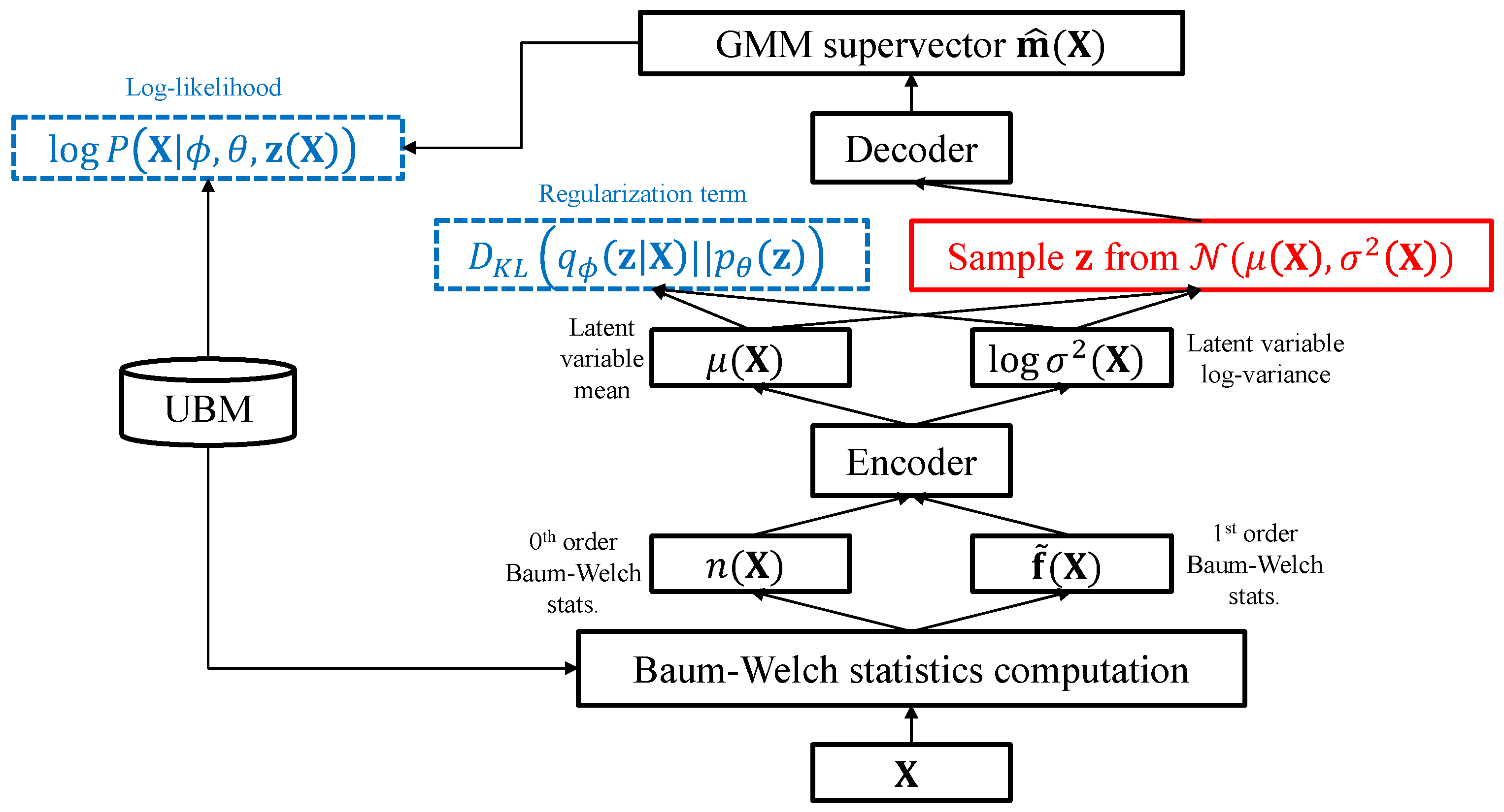
where $\mathbf{g}$ is a non-linear function which transforms the hidden variable $\mathbf{z}\left(\mathbf{X}\right)$ to the adaptation factor representing the variability of the ideal GMM supervector $\mathbf{m}\left(\mathbf{X}\right)$. In order to find the optimal function $\mathbf{g}$ and the hidden variable $\mathbf{z}\left(\mathbf{X}\right)$, we apply a VAE model consisting of an encoder and a decoder network as shown in Figure 1. In the proposed VAE architecture, the encoder network outputs an estimate of the hidden variable and the decoder network serves as the non-linear mapping function $\mathbf{g}$.

Analogous to the i-vector adaptation framework, the main task of the proposed VAE architecture is to generate a GMM so as to maximize the likelihood given the Baum–Welch statistics of the utterance. The encoder of the proposed system serves as a non-linear variability factor extraction model. Similar to the i-vector extractor, the encoder network takes the 0^th and 1^st-order Baum–Welch statistics of a given utterance $\mathbf{X}$ as input and generates the parametric distribution of the latent variable. The latent variable $\mathbf{z}$ is assumed to be a random variable following a Gaussian distribution, and each component of $\mathbf{z}$ is assumed to be uncorrelated with each other. In order to infer the distribution of the latent variable $\mathbf{z}\left(\mathbf{X}\right)$, it is sufficient for the encoder to generate the mean and the variance of $\mathbf{z}\left(\mathbf{X}\right)$. The decoder of the proposed system acts as the GMM adaptation model, generating the GMM supervector from the given latent variable according to the maximum likelihood criterion.

4.1. Maximum Likelihood Training

Once the GMM supervector $\widehat{\mathbf{m}}\left(\mathbf{X}\right)$ is generated at the output layer of the decoder, the log-likelihood conditioned on the latent variable $\mathbf{z}\left(\mathbf{X}\right)$ can be defined in a similar manner with (4) as:

$$\begin{array}{c}logP\left(\mathbf{X}\right|\varphi ,\theta ,\mathbf{z}\left(\mathbf{X}\right))=\sum _{c=1}^C(n_c\left(\mathbf{X}\right)log\frac{1}{{\left(2\pi \right)}^{F/2}{|{\mathbf{\Sigma }}_c}^{1/2}}\\ -\frac{1}{2}\sum _{l=1}^L{\gamma }_l\left(c\right){({\mathbf{x}}_l-{\widehat{\mathbf{m}}}_c\left(\mathbf{X}\right))}^t{\mathbf{\Sigma }}_c^{-1}({\mathbf{x}}_l-{\widehat{\mathbf{m}}}_c\left(\mathbf{X}\right))),\end{array}$$

(13)

where ${\widehat{\mathbf{m}}}_c\left(\mathbf{X}\right)$ denotes the $c^{\mathrm{th}}$ component of $\widehat{\mathbf{m}}\left(\mathbf{X}\right)$. Using Jensen’s inequality, the lower bound of the marginal log-likelihood can be obtained as follows:

$$\begin{array}{cc}\hfill logP\left(\mathbf{X}\right|\varphi ,\theta )=& log{\mathbb{E}}_{\mathbf{z}}\left[P\left(\mathbf{X}\right|\varphi ,\theta ,\mathbf{z})\right]\hfill \\ & \ge {\mathbb{E}}_{\mathbf{z}}[logP\left(\mathbf{X}\right|\varphi ,\theta ,\mathbf{z})].\hfill \end{array}$$

(14)

The marginal log-likelihood can be indirectly maximized by maximizing the expectation of the conditioned log-likelihood (13) with respect to the latent variable $\mathbf{z}$. The reparameterization trick in [19] can be utilized to compute the Monte Carlo estimate of the log-likelihood lower bound as given by

$${\mathbb{E}}_{\mathbf{z}}[logP\left(\mathbf{X}\right|\varphi ,\theta ,\mathbf{z})]\simeq \frac{1}{S}\sum _{s=1}^{S}logP\left(\mathbf{X}\right|\varphi ,\theta ,{\mathbf{z}}_s\left(\mathbf{X}\right)),$$

(15)

where S is the number of samples used for estimation and ${\mathbf{z}}_s\left(\mathbf{X}\right)$ is the reparameterized latent variable defined as follows:

$${\mathbf{z}}_s\left(\mathbf{X}\right)=\mu \left(\mathbf{X}\right)+\sigma \left(\mathbf{X}\right){ϵ}_s.$$

(16)

In (16), ${ϵ}_s\sim \mathcal{N}(0,\mathbf{I})$ is an auxiliary noise variable, and $\mu \left(\mathbf{X}\right)$ and $\sigma \left(\mathbf{X}\right)$ are respectively the mean and standard deviation of the latent variable $\mathbf{z}\left(\mathbf{X}\right)$ generated from the encoder network. By replacing the reconstruction error term of the VAE objective function (11) with the estimated log-likelihood lower bound, the objective function of the proposed system can be written as:

$$\begin{array}{cc}\hfill E_{Prop}\left(\mathbf{X}\right)=& D_{\mathit{KL}}(q_{\varphi }\left(\mathbf{z}\right|\mathbf{X})\Vert p_{\theta }\left(\mathbf{z}\right))\hfill \\ & -\frac{1}{S}\sum _{s=1}^{S}logP\left(\mathbf{X}\right|\varphi ,\theta ,{\mathbf{z}}_s\left(\mathbf{X}\right)).\hfill \end{array}$$

(17)

From (17), it is seen that the proposed VAE is trained not only to maximize the similarity between the prior and posterior distributions of the latent variable, but also to maximize the log-likelihood of the generated GMM by minimizing $E_{Prop}$ via error back-propagation. Moreover, we assume that the prior distribution for $\mathbf{z}$ is $p_{\theta }\left(\mathbf{z}\right)=\mathcal{N}\left(\mathbf{z}\right|0,\mathbf{I})$ analogous to the prior for $\mathbf{w}$ in the i-vector framework.

4.2. Non-Linear Feature Extraction and Speaker Verification

The encoder network of the proposed VAE generates the latent variable mean $\mu \left(\mathbf{X}\right)$ and the log-variance $log{\sigma }^2\left(\mathbf{X}\right)$. Once the VAE has been trained, the encoder network is used as a feature extraction model, as shown in Figure 2. Similar to the conventional i-vector extractor, the encoder network takes the Baum–Welch statistics of the input speech utterance and generates a random variable with a Gaussian distribution, which contains essential information for modeling an utterance-dependent GMM. The mean of the latent variable $\mu \left(\mathbf{X}\right)$ is exploited as a compact representation of the variability within the GMM distribution dependent on $\mathbf{X}$. Moreover, since the variance of the latent variable ${\sigma }^2\left(\mathbf{X}\right)$ represents the variability of the distribution, it is used as a proxy for the uncertainty caused by the short duration of the given speech samples. The features extracted by the proposed VAE can be transformed via feature compensation techniques (e.g., linear discriminant analysis (LDA) [1]) in order to improve the discriminability of the features.

Given a set of $N\left(p\right)$ enrollment speech samples spoken by an arbitrary speaker p

$$\mathbf{X}\left(p\right)=\{{\mathbf{X}}_1\left(p\right),{\mathbf{X}}_2\left(p\right),\cdots ,{\mathbf{X}}_{N\left(p\right)}\left(p\right)\},$$

(18)

the speaker model for p is obtained by averaging the features extracted from each speech sample. To determine whether a test utterance ${\mathbf{X}}_{test}$ is spoken by the speaker p, analogous to the i-vector framework, probabilistic linear discriminant analysis (PLDA) is used to compute the similarity between the feature extracted from ${\mathbf{X}}_{test}$ and the speaker model of p.

Unlike the conventional i-vector framework, which only uses the mean of the latent variable as feature, the proposed scheme utilizes both the mean and variance of the latent variable to take the uncertainty into account. Providing the speaker decision model (e.g., PLDA) with information about the uncertainty within the input speech, which is represented by the variance of the latent variable, may improve the speaker recognition performance. This is verified in the experiments shown in Section 5.

5. Experiments

5.1. Databases

In order to evaluate the performance of the proposed technique in the random digit speaker verification task, a set of experiments was conducted using the TIDIGITS dataset. The TIDIGITS dataset contains 25,096 clean utterances spoken by 111 male and 114 female adults, and by 50 boys and 51 girls [25]. For each of the 326 speakers in the TIDIGITS dataset, a set of isolated digits and 2–7 digit sequences were spoken. The TIDIGITS dataset was split into two subsets, each containing 12,548 utterances from all 326 speakers, and they were separately used as the enrollment and trial data. In the TIDIGITS experiments, the TIMIT dataset [26] was used for training the UBM, total variability matrix, and the embedding networks.

5.2. Experimental Setup

For the experimented systems, the acoustic feature involves 19-dimensional MFCCs and the log-energy extracted every 10 ms, using a 20 ms Hamming window via the SPro library [27]. Together with the delta (first derivative) and delta-delta (second derivative) of the 19-dimensional MFCCs and the log-energy, the frame-level acoustic feature used in our experiments was given by a 60-dimensional vector.

We trained the UBM containing 32 mixture components in a gender- and age-independent manner, using all the speech utterances in the TIMIT dataset. Training the UBM, total variability matrix, and the i-vector extraction was done by using the MSR Identity Toolbox via MATLAB [28]. The encoders and decoders of the VAEs were configured to have a single hidden layer with 4096 rectified linear unit (ReLU) nodes, and the dimensionality of the latent variables was set to be 200. The implementation of the VAEs was done using Tensorflow [29] and trained using the AdaGrad optimization technique [30]. Additionally, dropout [31] with a fraction of 0.8 and L2 regularization with a weight of 0.01 were applied for training all the VAEs, and the Baum–Welch statistics extracted from the entire TIMIT dataset were used as training data. A total of 100 samples were used for the reparameterization shown in (15).

For all the extracted utterance-level features, linear discriminant analysis (LDA) [1] was applied for feature compensation, and the dimensionality was finally reduced to 200. PLDA [32] was used for speaker verification, and the speaker subspace dimension was set to be 200.

Four performance measures were evaluated in our experiments: classification error (Class. err.), EER, minimum NIST SRE 2008 DCF (DCF08), and minimum NIST SRE 2010 DCF (DCF10). The classification error was measured while performing a speaker identification task where each trial utterance was compared with all the enrolled speakers via PLDA, and the enrolled speaker with the highest score was chosen as the identified speaker. Then, the ratio of the number of wrongly classified trial samples to the total number of trial samples represented the classification error. The EER and minimum DCFs are widely used measures for speaker verification, where the EER indicates the error when the false positive rate (FPR) and the false negative rate (FNR) are the same [1], and the minimum DCFs represent the decision cost obtained with different weights to FPR and FNR. The parameters for measuring DCF08 and DCF10 were chosen according to the weights given by the NIST SRE 2008 [33] and the NIST SRE 2010 [34] protocols, respectively.

5.3. Effect of the Duration on the Latent Variable

In order to investigate the ability of the latent variable to capture the uncertainty caused by short duration, the differential entropies (the differential entropy—or the continuous random variable entropy—measures the average uncertainty of a random variable) of the latent variables were computed. Since the latent variable $\mathbf{z}\left(\mathbf{X}\right)$ in the proposed VAE has a Gaussian distribution, the differential entropy can be formulated as follows:

$$h\left(\mathbf{z}\left(\mathbf{X}\right)\right)=\frac{1}{2}log{\left(2\pi e\right)}^K+\frac{1}{2}log\prod _{k=1}^K{\sigma }_k^2\left(\mathbf{X}\right).$$

(19)

In (19), K represents the dimensionality of the latent variable and ${\sigma }_k^2\left(\mathbf{X}\right)$ is the $k^{\mathrm{th}}$ element of ${\sigma }^2\left(\mathbf{X}\right)$. From each speech sample in the entire TIDIGITS dataset, 200-dimensional latent variable variance was generated using the encoder network of the proposed framework and used for computing the differential entropy.

In Figure 3, the differential entropies averaged in six different duration groups (i.e., less than 1 s, 1–2 s, 2–3 s, 3–4 s, 4–5 s, and more than 5 s) are shown. As can be seen in the result, the differential entropy computed using the variance of the latent variable gradually decreased as the duration increased. Despite a rather small time difference between the first duration group (i.e., less than 1 s) and the sixth duration group (i.e., more than 5 s), the relative decrement in entropy was 29.91%. This proves that the latent variable variance extracted from the proposed system was capable of indicating the uncertainty caused by the short duration.

5.4. Experiments with VAEs

To verify the performance of the proposed VAE trained with the log-likelihood-based reconstruction error function, we conducted a series of speaker recognition experiments on the TIDIGITS dataset. For performance comparison, we also applied various feature extraction approaches. The approaches compared with each other in these experiments were as follows:

• I-vector: standard 200-dimensional i-vector;
• Autoencode: VAE trained to minimize the cross-entropy between the input Baum–Welch statistics and the reconstructed output Baum–Welch statistics;
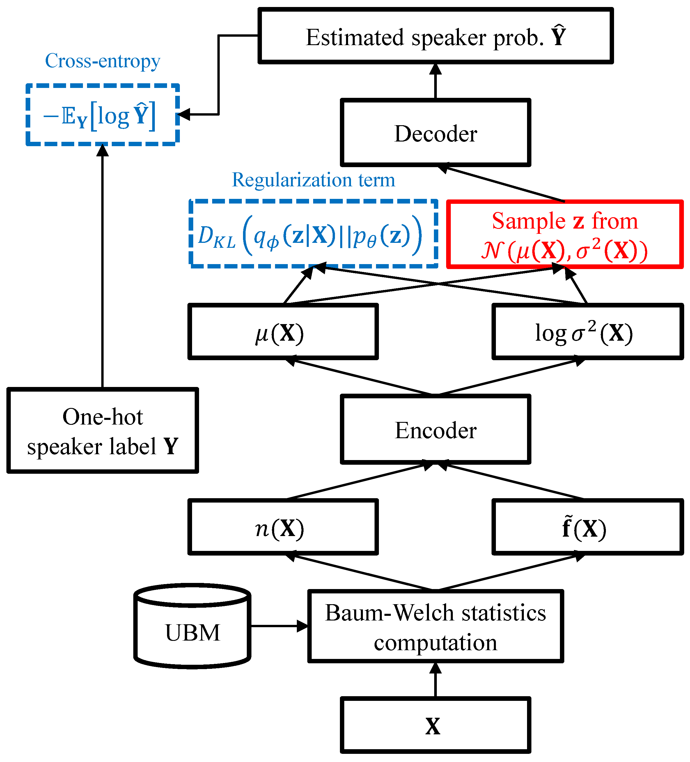
• Classify: VAE trained to minimize the cross-entropy between the softmax output and the one-hot speaker label;
• Proposed: the proposed VAE trained to minimize the negative log-likelihood-based reconstruction error.

Autoencode is a standard VAE for reconstructing the input at the output, and was trained to minimize $E_{\mathit{VAE}}$ (11) given the Baum–Welch statistics as input. On the other hand, Classify is a VAE for estimating the speaker label, which was trained to minimize the following loss function:

$$\begin{array}{cc}\hfill E_{\mathit{Class}}\left(\mathbf{x}\right)=& D_{\mathit{KL}}(q_{\varphi }\left(\mathbf{z}\right|\mathbf{x})\Vert p_{\theta }\left(\mathbf{z}\right))-{\mathbb{E}}_{\mathbf{Y}}[log\widehat{\mathbf{Y}}],\hfill \end{array}$$

(20)

where $\mathbf{Y}$ denotes the one-hot speaker label of utterance $\mathbf{X}$ and $\widehat{\mathbf{Y}}$ is the softmax output of the decoder network. The network structure for Classify is depicted in Figure 4. In this experiment, only the mean vectors of the latent variables were used for Autoencode, Classify, and Proposed.

The results shown in

Table 1. Comparison of results between using the i-vector and the mean latent variables extracted from VAEs trained for different tasks. Class. Err.: classification error; DCF08: minimum NIST SRE 2008 DCF; DCF10: minimum NIST SRE 2010 DCF; EER: equal error rate.

	Class. Err. (%)	EER (%)	DCF08	DCF10
i-vector	12.62	3.36	2.00	0.07
Autoencode	24.59	6.06	2.69	0.09
Classify	40.01	8.13	4.21	0.10
Proposed	11.89	3.61	2.09	0.07

tell us that the VAEs trained with the conventional criteria (i.e., Autoencode and Classify) performed poorly compared to the standard i-vector. On the other hand, the proposed VAE with likelihood-based reconstruction error was shown to provide better performance for speaker recognition than the other methods. The feature extracted using the VAE trained with the proposed criterion provided comparable verification performance (i.e., EER, DCF08, DCF10) to the conventional i-vector feature. Moreover, in terms of classification, the proposed framework outperformed the i-vector framework with a relative improvement of 5.8% in classification error. Figure 5 shows the detection error tradeoff (DET) curves obtained from the four tested approaches.

5.5. Feature-Level Fusion of I-Vector and Latent Variable

In this subsection, we tested the features obtained by augmenting the conventional i-vector with the mean and variance of the latent variable extracted from the proposed VAE. For performance comparison, we applied the following six different feature sets:

• I-vector(400): standard 400-dimensional i-vector;
• I-vector(600): standard 600-dimensional i-vector;
• LM+LV: concatenation of the 200-dimensional latent variable mean and the log-variance, resulting in a 400-dimensional vector;
• I-vector(200)+LM: concatenation of the 200-dimensional i-vector and the 200-dimensional latent variable mean, resulting in a 400-dimensional vector;
• I-vector(200)+LV: concatenation of the 200-dimensional i-vector and the 200-dimensional latent variable log-variance, resulting in a 400-dimensional vector;
• I-vector(200)+LM+LV: concatenation of the 200-dimensional i-vector and the 200-dimensional latent variable mean and log-variance, resulting in a 600-dimensional vector.

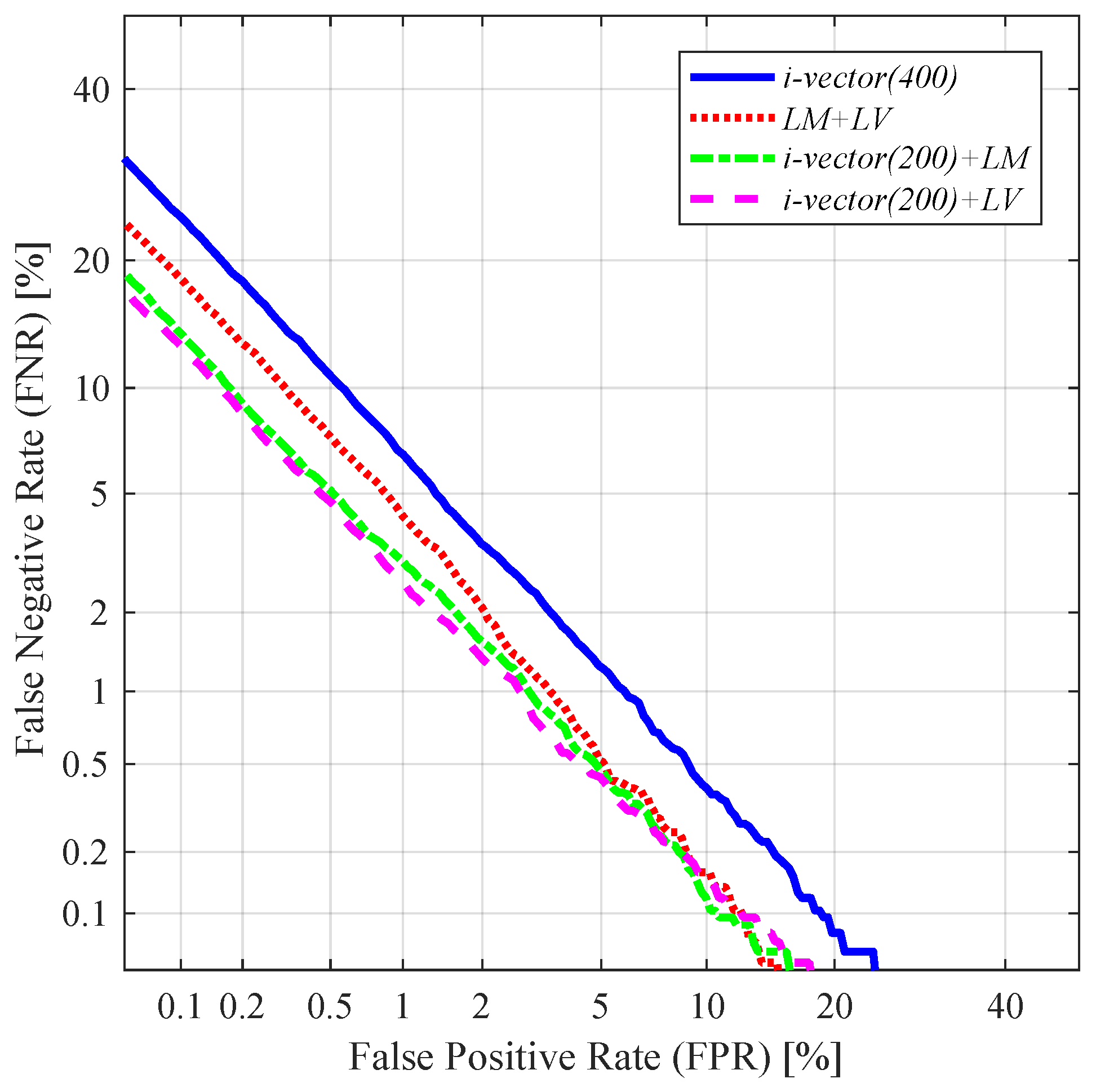
As seen from

Table 2. Comparison of results between various feature-level fusions of the conventional i-vector and mean and log-variance of the latent variable extracted from the proposed VAE.

ine	Class. Err. (%)	EER (%)	DCF08	DCF10
i-vector(400)	7.67	2.68	1.54	0.06
LM + LV	6.94	2.03	1.23	0.05
i-vector(200) + LM	5.36	1.78	0.97	0.05
i-vector(200) + LV	4.99	1.65	0.94	0.04
i-vector(600)	5.07	2.17	1.29	0.05
i-vector(200) + LM + LV	2.75	0.97	0.61	0.03

and Figure 6, the augmentation of the latent variable greatly improved the performance in all the tested cases.

By using only the mean and log-variance of the latent variable together (i.e., LM+LV), a relative improvement of 24.25% was achieved in terms of EER, compared to the conventional i-vector with the same dimension (i.e., i-vector(400)). The concatenation of the standard i-vector and the latent variable mean (i.e., i-vector(200)+LM) also improved the performance. Especially in terms of EER, i-vector(200)+LM achieved a relative improvement of 33.58% compared to i-vector(400). This improvement may be attributed to the non-linear feature extraction process. Since the latent variable mean is trained to encode the various variability within the distributive pattern of the given utterance via a non-linear process, it may contain information that is not obtainable from the linearly extracted i-vector. Thus, by supplementing the information ignored by the i-vector extraction process, a better representation of the speech can be obtained.

The best verification and identification performance out of all the 400-dimensional features (i.e., i-vector(400), LM+LV, i-vector(200)+LM, and i-vector(200)+LV) was obtained when concatenating the standard i-vector and the latent variable log-variance (i.e., i-vector(200)+LV). I-vector(200)+LV achieved a relative improvement of 38.43% in EER and 34.94% in classification error compared to i-vector(400). This may have been due to the capability of the latent variable variance of capturing the amount of uncertainty, which allows the decision score to take advantage of the duration dependent reliability.

Concatenating the standard i-vector with both the mean and log-variance of the latent variable (i.e., i-vector(200)+LM+LV) further improved the speaker recognition performance. Using the i-vector(200)+LM+LV achieved a relative improvement of 55.30% in terms of EER, compared to the standard i-vector with the same dimension (i.e., i-vector(600)). Figure 7 shows the DET curves obtained when i-vector(200)+LM+LV and i-vector(600) were applied.

5.6. Score-Level Fusion of I-Vector and Latent Variable

In this subsection, we present the experimental results obtained from a speaker recognition task where the decision was made by fusing the PLDA scores of i-vector features and VAE-based features. Given a set of independently computed PLDA scores $S_r$, $r=1,\cdots ,R$, the fused score $S_{fused}$ was computed by simply adding them as

$$S_{fused}=\sum _{r=1}^R{S}_r.$$

(21)

We compared the following scoring schemes:

• I-vector: PLDA score obtained by using the standard 200-dimensional i-vector;
• LM: PLDA score obtained by using the 200-dimensional latent variable mean;
• LV: PLDA score obtained by using the 200-dimensional latent variable log-variance;
• I-vector+LM: fusion of the PLDA scores obtained by using the 200-dimensional i-vector and the 200-dimensional latent variable mean;
• I-vector+LV: fusion of the PLDA scores obtained by using the 200-dimensional i-vector and the 200-dimensional latent variable log-variance;
• LM+LV: fusion of the PLDA scores obtained by using the latent variable mean and log-variance;
• I-vector+LM+LV: fusion of the PLDA scores obtained by using the standard 200-dimensional i-vector and the 200-dimensional latent variable mean and log-variance.

Table 3. Comparison of results between various score-level fusions of the conventional i-vector and the mean and log-variance of the latent variable extracted from the proposed VAE.

	Class. Err. (%)	EER (%)	DCF08	DCF10
i-vector	12.62	3.36	2.00	0.07
LM	11.89	3.61	2.09	0.07
LV	17.78	4.65	2.57	0.08
i-vector+LM	7.03	2.63	1.63	0.06
ine i-vector+LV	7.39	2.76	1.69	0.06
LM+LV	10.26	3.50	2.02	0.07
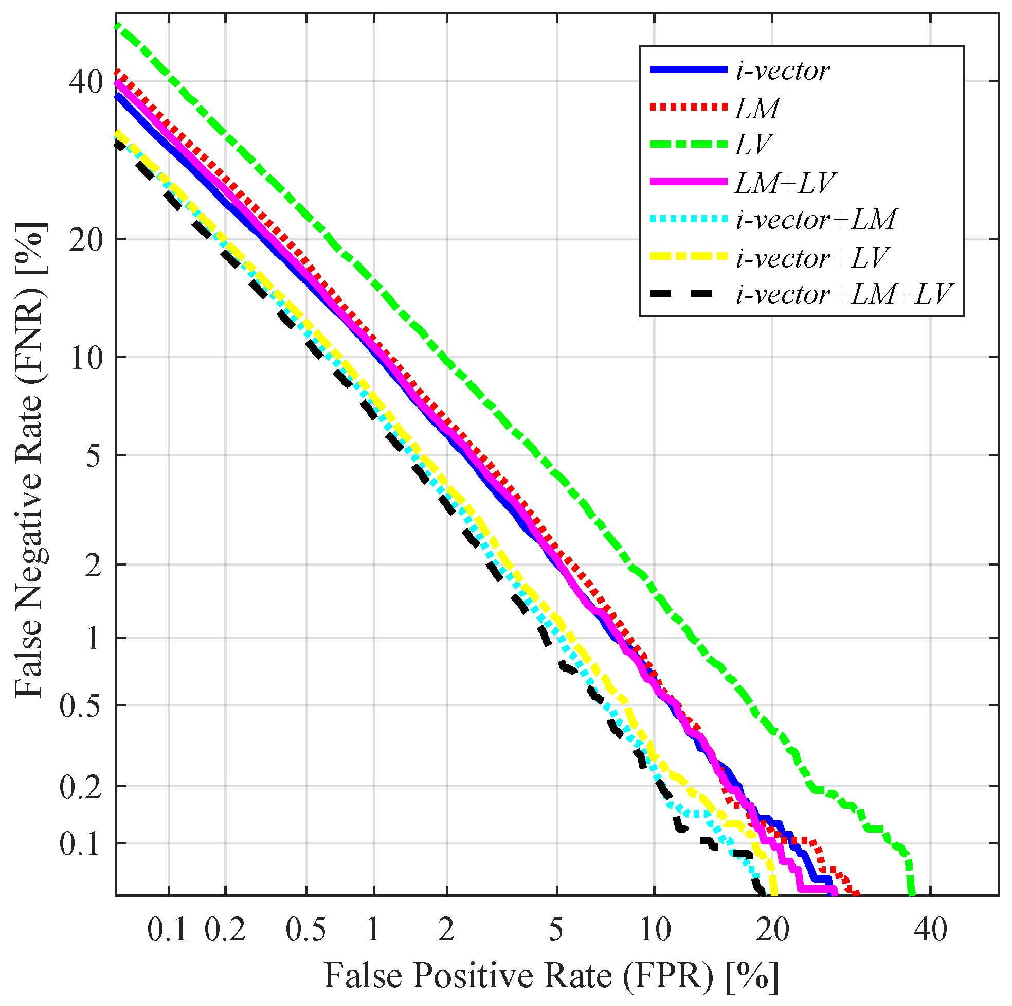
i-vector+LM+LV	5.75	2.49	1.57	0.06

and Figure 8 give the results obtained through these scoring schemes. As shown in the results, using the latent variable mean and log-variance vectors as standalone features yielded comparable performance to the conventional i-vector method (i.e., LM and LV). Additionally, fusing the latent-variable-based scores with the score provided by the standard i-vector feature further improved the performance (i.e., i-vector+LM and i-vector+LV). The best score-level fusion performance was obtained by fusing all the scores obtained by the standard i-vector and the latent variable mean and log-variance vector (i.e., i-vector+LM+LV), achieving a relative improvement of 25.89% in terms of EER compared to i-vector. However, the performance improvement produced by the score-level fusion methods was relatively smaller than the feature-level fusion methods presented in Table 2. This may have been because the score-level fusion methods compute the scores of the i-vector and the latent variable-based features independently, and as a result the final score cannot be considered an optimal way to utilize their joint information.

6. Conclusions

In this paper, a novel unsupervised deep-learning model-based utterance-level feature extraction for speaker recognition was proposed. In order to capture the variability that has not been fully represented by the linear projection in the traditional i-vector framework, we designed a VAE for GMM adaptation and exploited the latent variable as the non-linear representation of the variability in the given speech. Analogous to the standard VAE, the proposed architecture is composed of an encoder and a decoder network, where the former estimates the distribution of the latent variable given the Baum–Welch statistics of the speech and the latter generates the ideal GMM supervector from the latent variable. Moreover, to take the uncertainty caused by short duration speech utterances into account while extracting the feature, the VAE is trained to generate a GMM supervector in such a way as to maximize the likelihood. The training stage of the proposed VAE uses a likelihood-based error function instead of the conventional reconstruction errors (e.g., cross-entropy).

To investigate the characteristics of the features extracted from the proposed system in a practical scenario, we conducted a set of random-digit sequence experiments using the TIDIGITS dataset. We observed that the variance of the latent variable generated from the proposed network apparently demonstrated the level of uncertainty which gradually decreased as the duration of the speech increased. Additionally, using the mean and variance of the latent variable as features provided comparable performance to the conventional i-vector and further improved the performance when used in conjunction with the i-vector. The best performance was achieved by feature-level fusion of the i-vector and the mean and variance of the latent variable.

In our future study, we will further develop training techniques for the VAE not only to maximize the likelihood but also to amplify the speaker discriminability of the generated latent variable.