A Simple Estimation Method of Weibull Modulus and Verification with Strength Data


Abstract
1. Introduction
2. Approximate Methods of Weibull Modulus Estimation
(for N = 20).
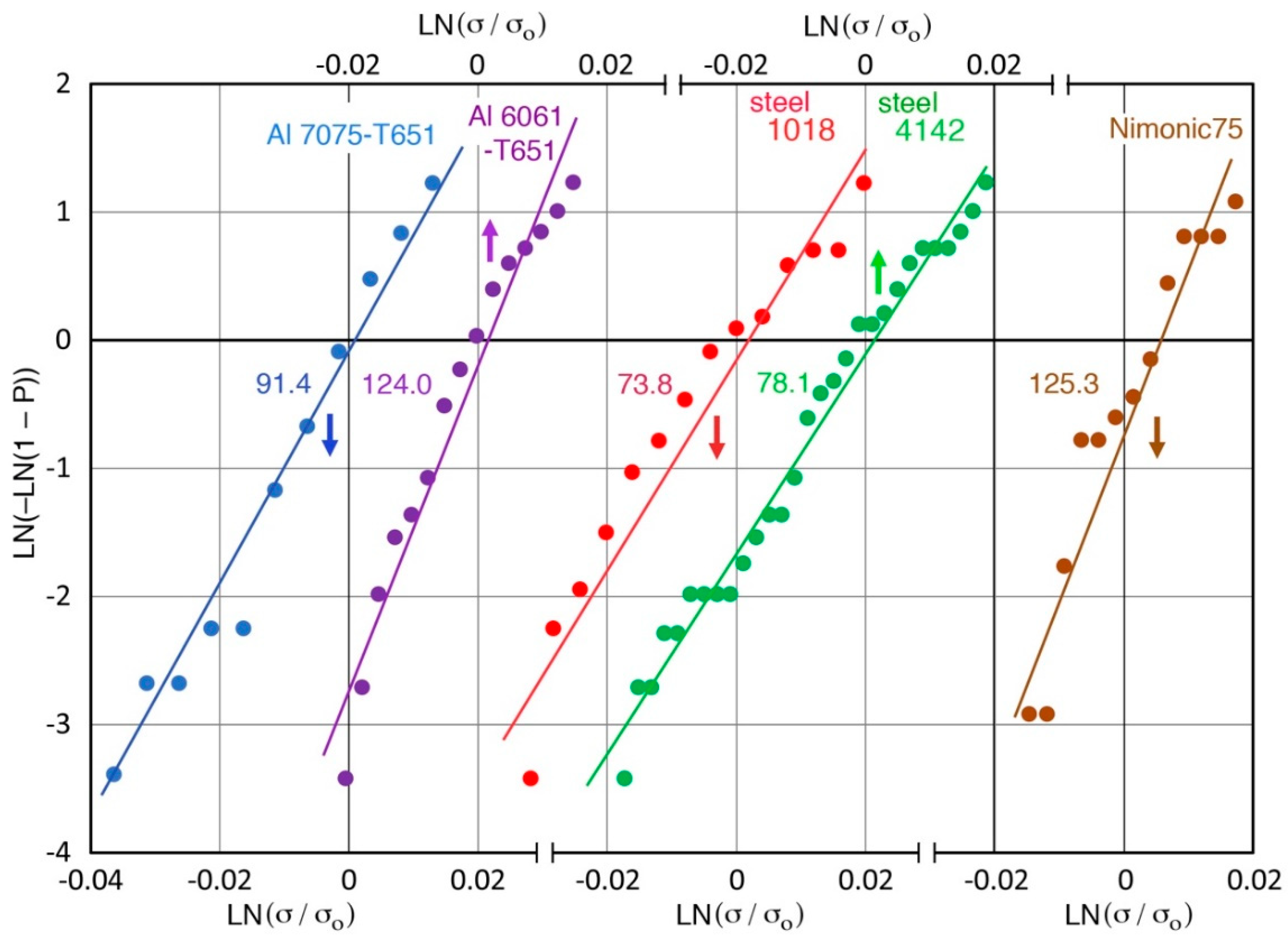
3. Weibull Moduli of Five Metal Alloys
4. Material Strength Data
4.1. Historic Wrought Iron and Steel
4.2. Metals and Alloys
4.3. Ceramics and Glasses
4.4. Fibers
4.5. Composites
4.6. Summary
5. Discussion
5.1. Estimation of m from Standard Deviation or from Coefficient of Variation
5.2. Industrial Strength Data
- a.
- Hot-rolled steel [129]
- b.
- Shipbuilding steels [130]
- c.
- Chinese HSLA steels [131]
- d.
- Plain carbon and HSLA steels, S235, S355, and S550 [132]
- e.
- Hot-rolled steels [133]
- f.
- Steel shapes [134]
- g.
- h.
- High strength suspension cable wires [15]
- i.
- Cast iron pipes [137]
- j.
- Graphite [138]
- k.
- Large-scale testing
6. Conclusions
- Methods of estimating Weibull modulus (m) of an experimentally obtained dataset were examined. These utilized the average (<σ>) and standard deviation (S) (or coefficient of variation, CV) based on the normal distribution. Several approximate relationships have been proposed starting from Robinson [11], but all of them deviate from the exact expression given with the gamma function.
- The exact expression can be represented by m = 1.271 <σ>/S = 1.271/CV with R2 = 0.9999. Robinson used 1.20 as the constant [11].
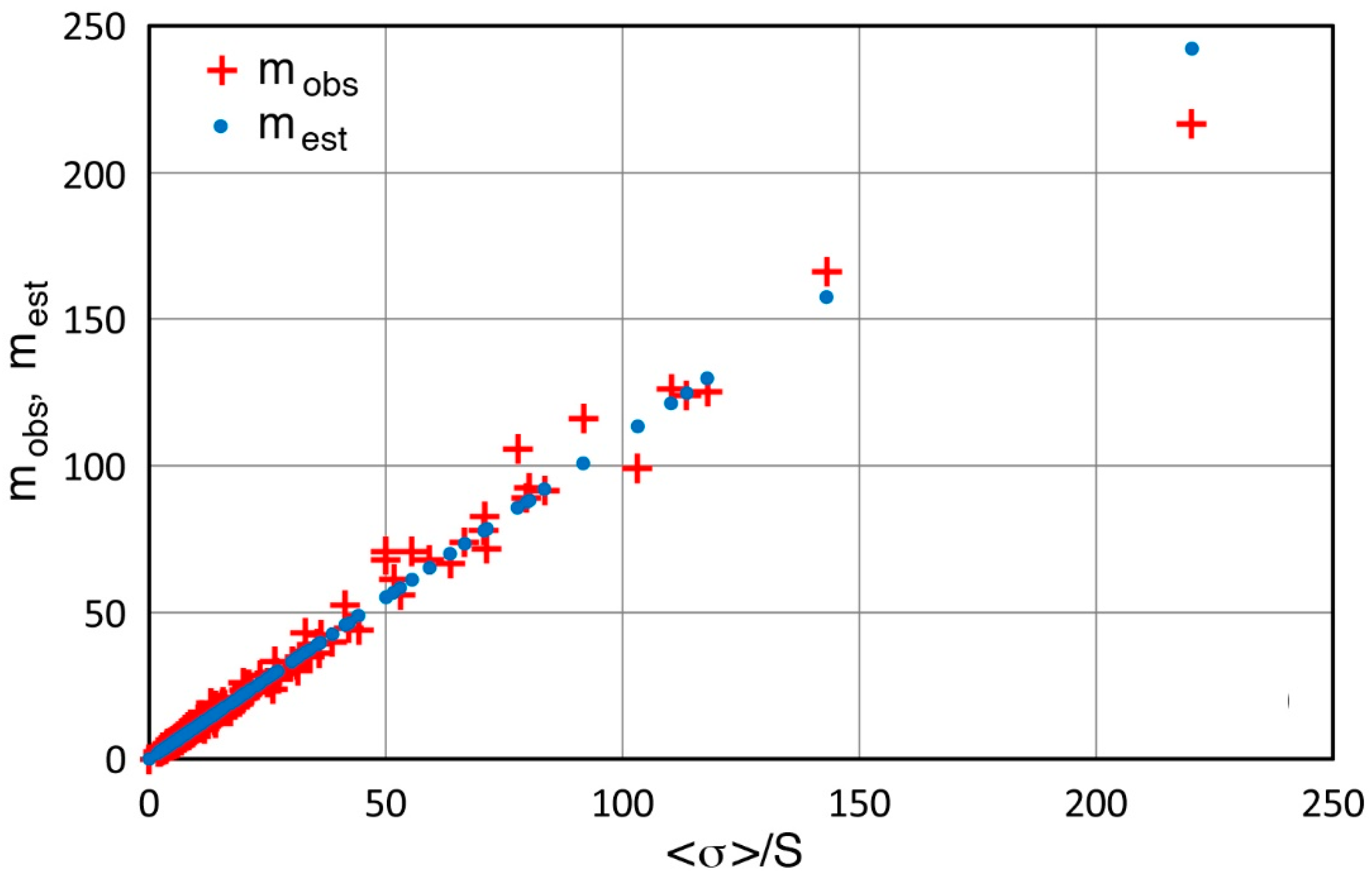
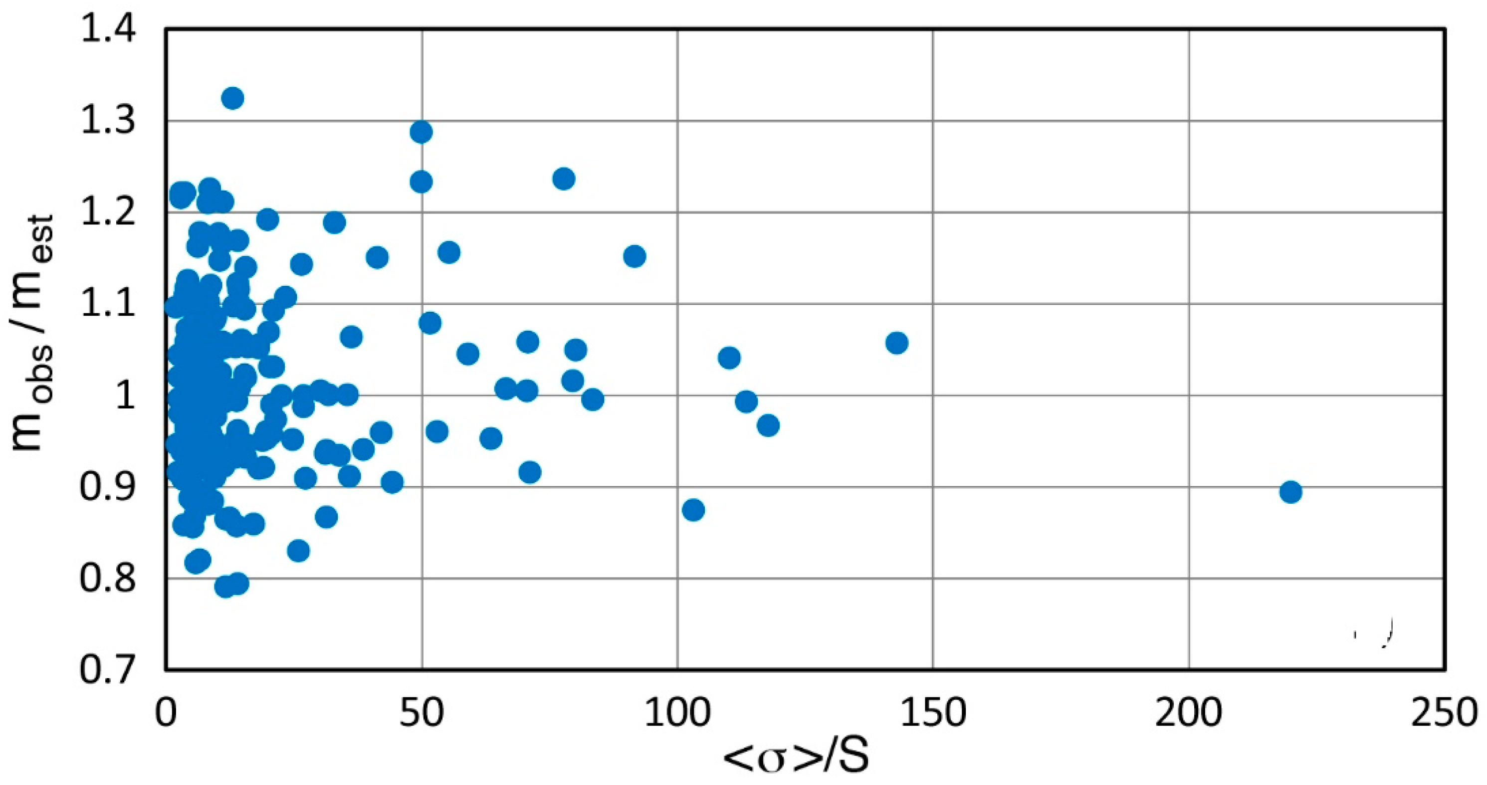
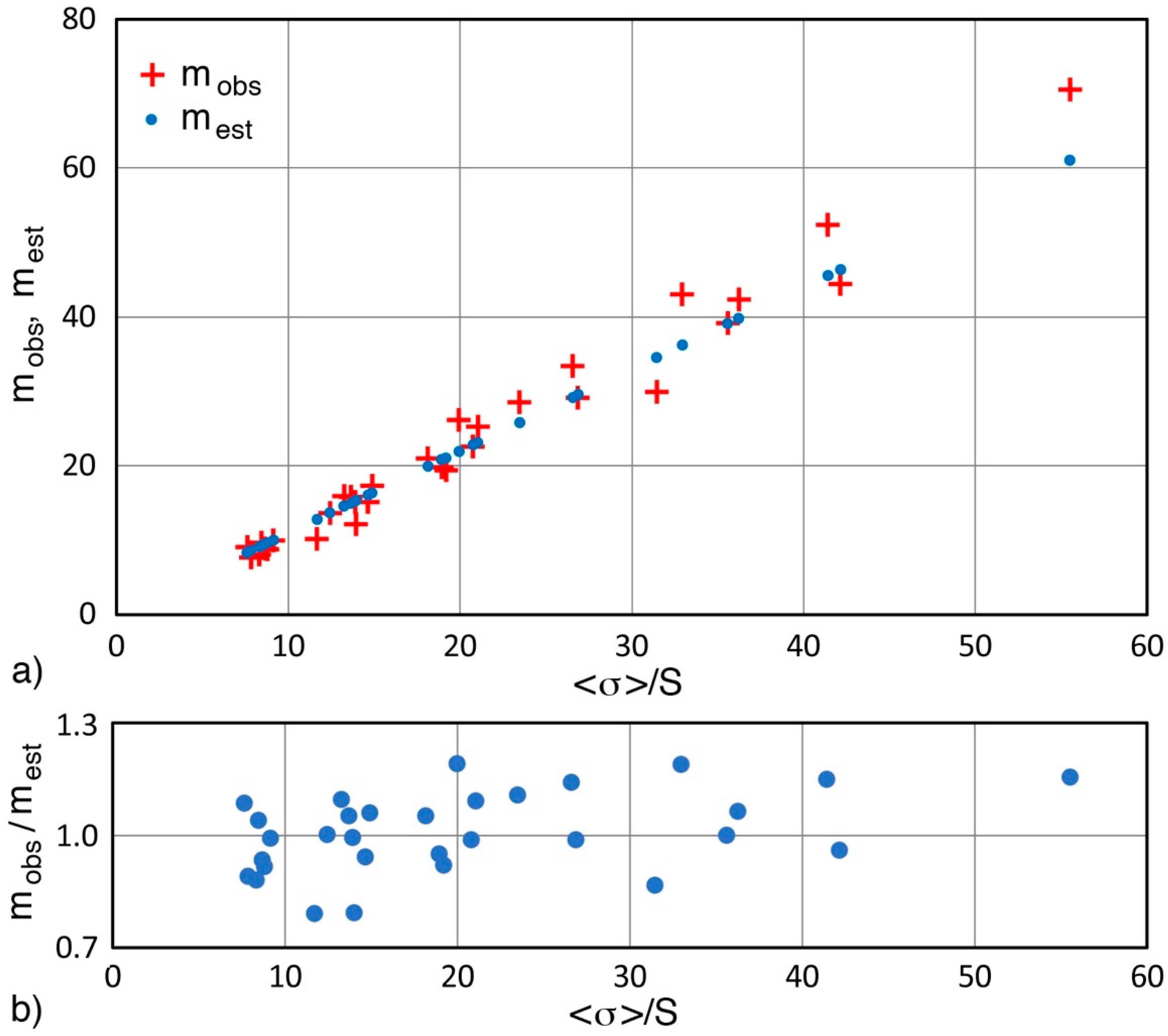
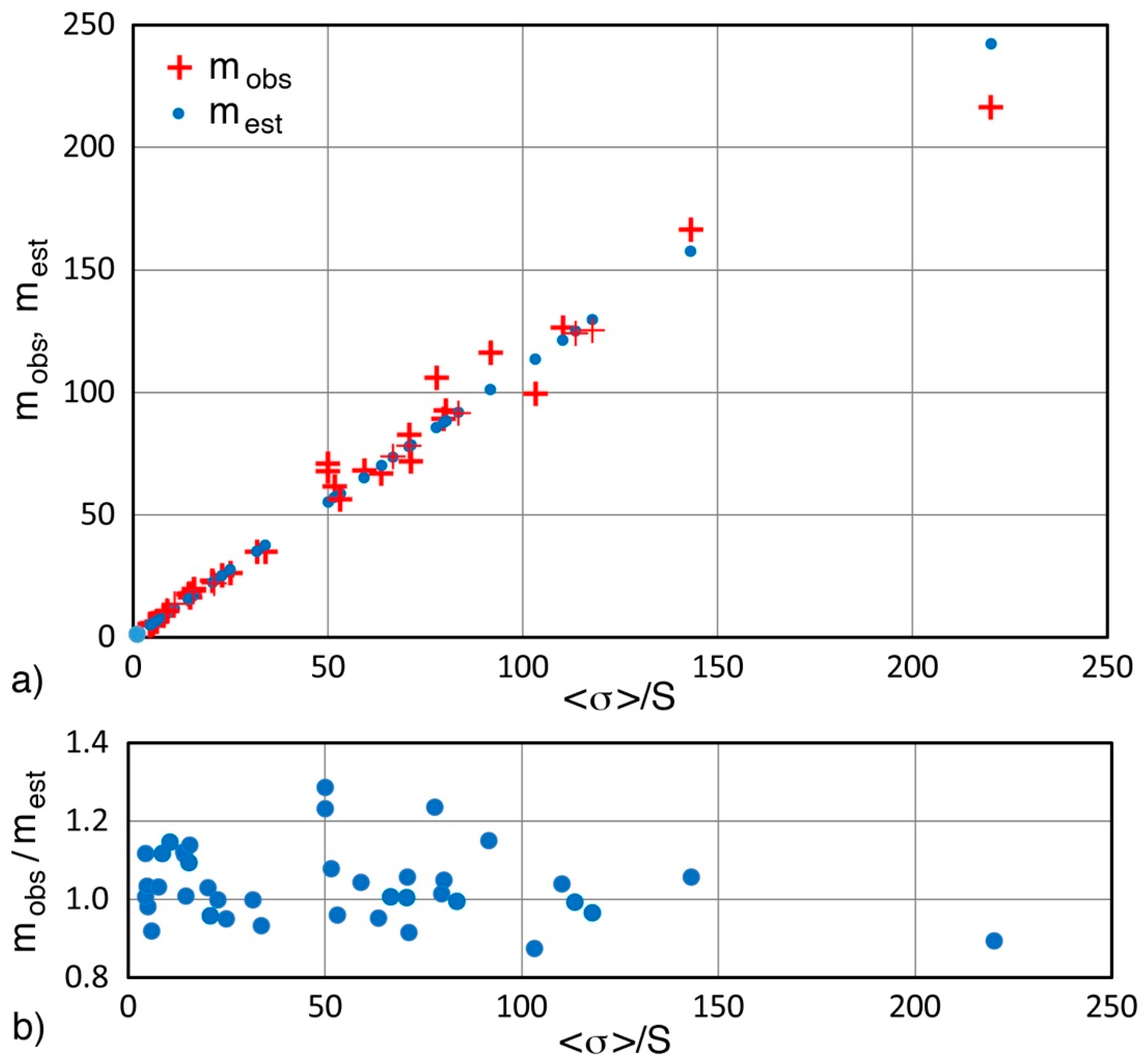
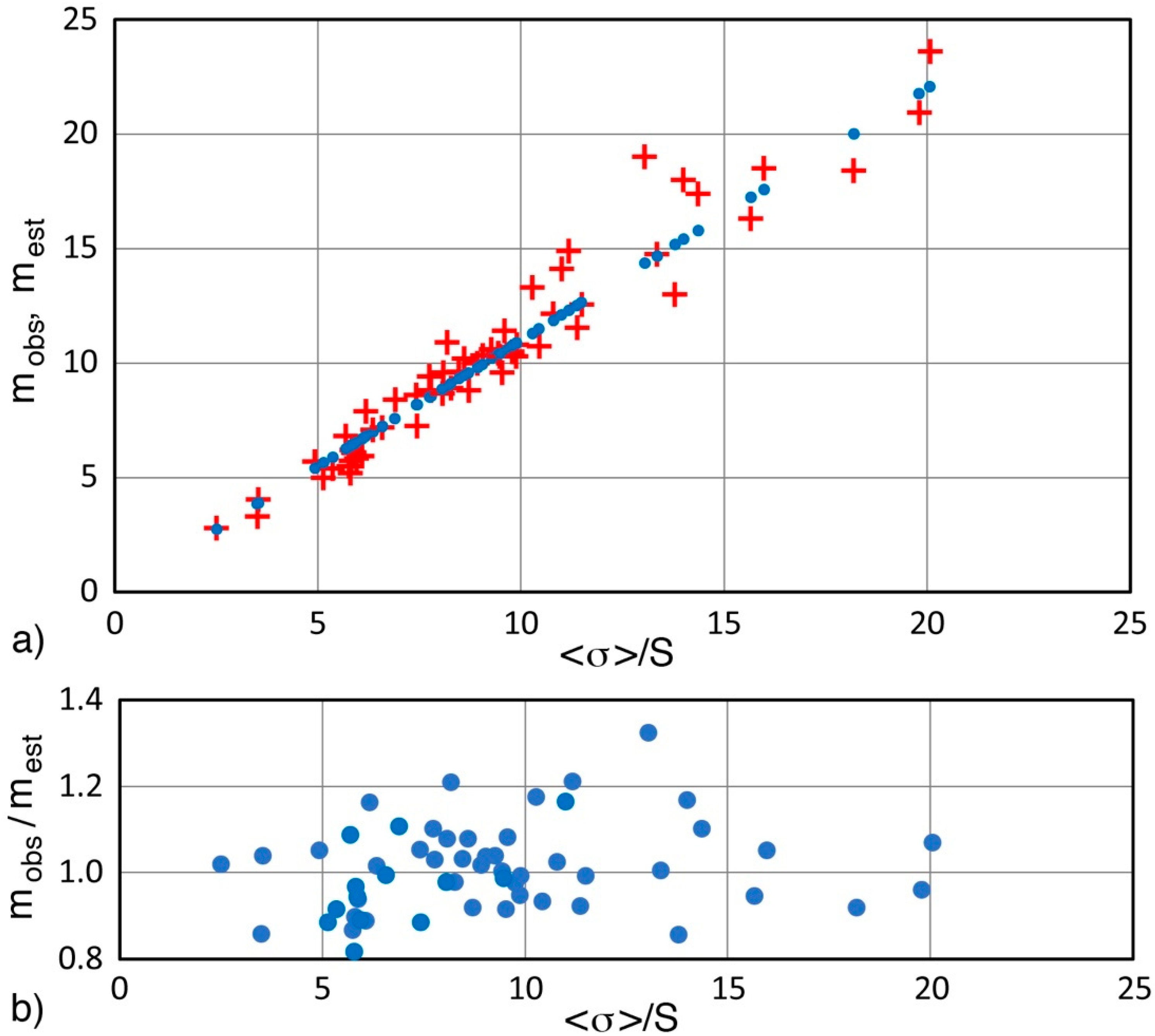
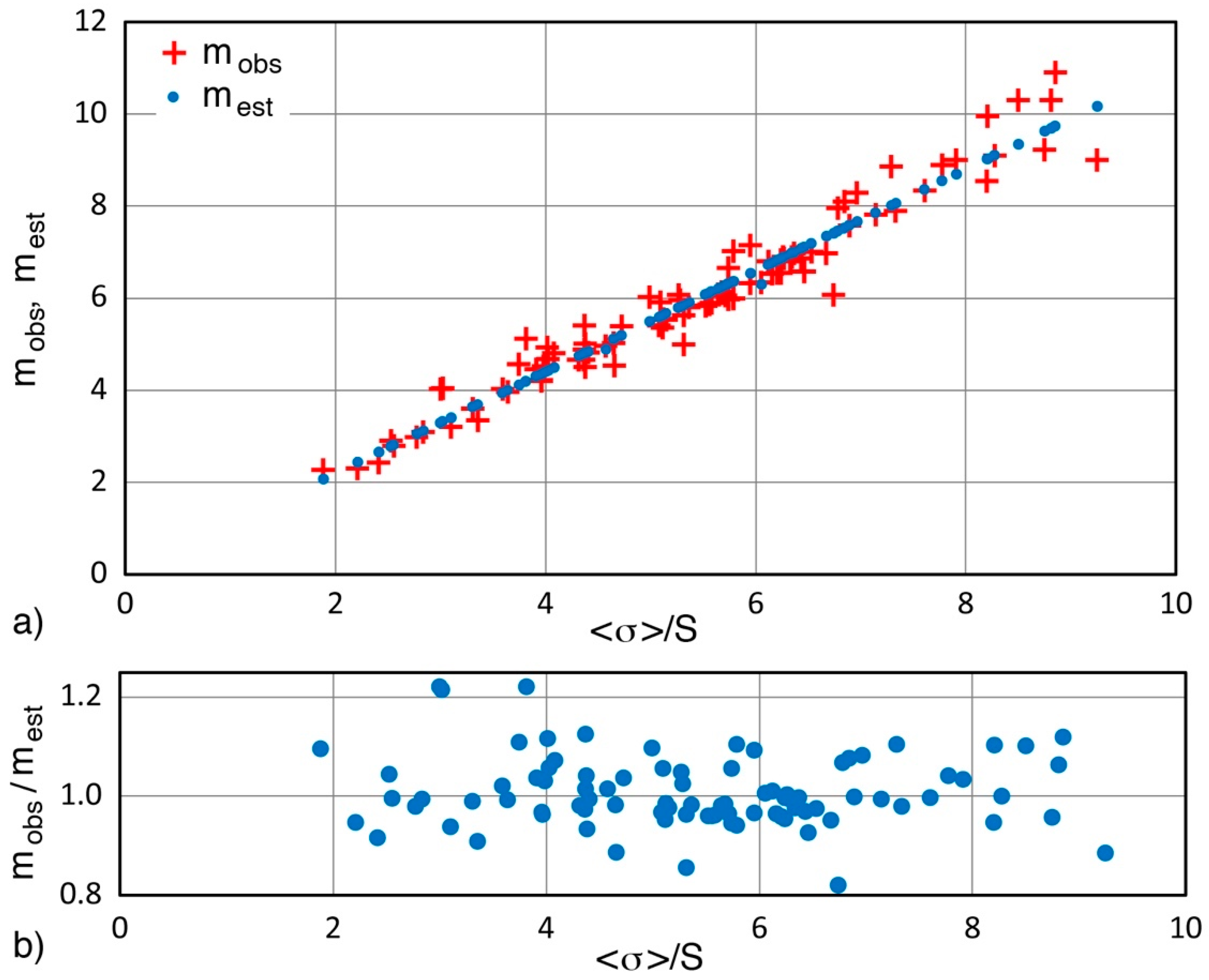
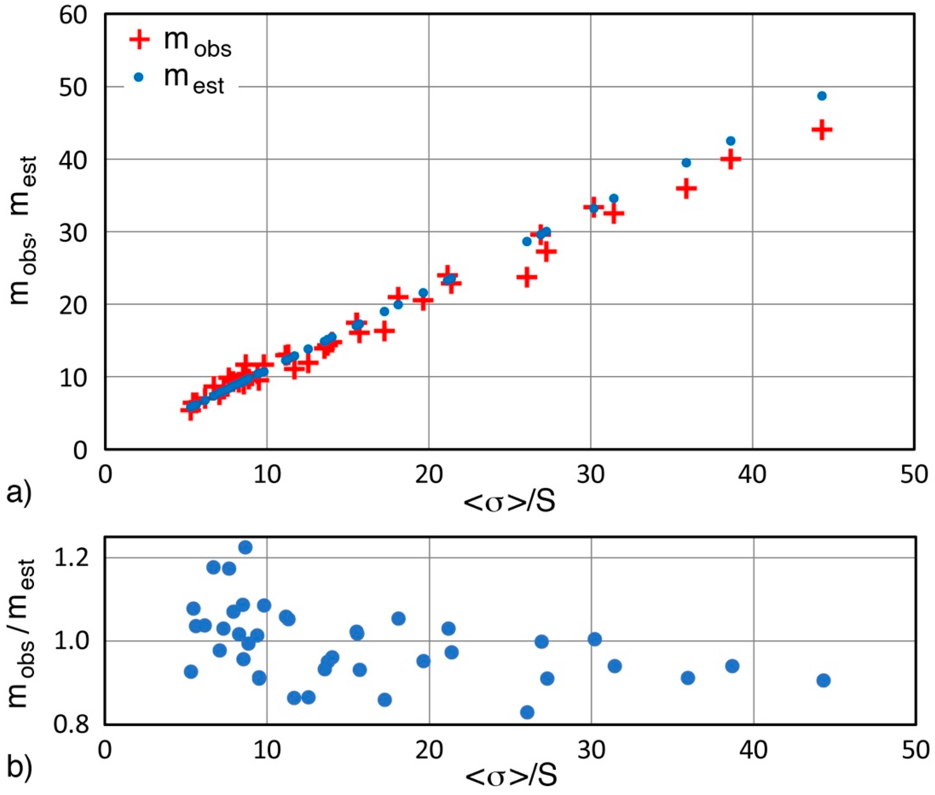
- In order to obtain m values that fit with the actually observed material strength datasets, a reduction of the constant from 1.271 to 1.10 is found to be optimal. This produces the modified Robinson relation of m = 1.10 <σ>/S = 1.10/CV, which can estimate m values that are in good agreement with the m values obtained from Weibull analyses. This agreement was verified by over 260 datasets of the strength of metals, ceramics, fibers, and composite materials, with most of the data from tensile or flexure testing.
- Applications of this simple estimation method are discussed. A common notion that ductile metals always have high m values must be discarded. Causes of m reduction need to be considered as material variation, and test accuracies can affect the outcomes. The method can add a quantitative tool based on the Weibull theory to engineering practice.
Funding
Acknowledgments
Conflicts of Interest
References
- Weibull, W. A statistical theory of the strength of material. Ing. Vetenskapa Acad. Handlingar 1939, 151, 1–45. [Google Scholar]
- Weibull, W. A statistical distribution function of wide applicability. Trans. ASME J. Appl. Mech. 1951, 73, 293–297. [Google Scholar]
- Lai, C.-D.; Pra Murthy, D.N.; Xie, M. Weibull Distributions and Their Applications. In Springer Handbook of Engineering Statistics; Pham, H., Ed.; Springer: Cham, Switzerland, 2006; pp. 63–78. [Google Scholar]
- Abernethy, R.B.; Breneman, J.E.; Medlin, C.H.; Reinman, G.L. Weibull Analysis Handbook; AFWAL-TR-83-2079; Pratt and Whitney Aircraft: North Palm Beach, FL, USA, 1983; 243p. [Google Scholar]
- Abernethy, R.B. The New Weibull Handbook, 2nd ed.; Gulf Pub. Co.: North Palm Beach, FL, USA, 1996; 350p. [Google Scholar]
- Song, K.W.; Chang, I.H.; Pham, H. A software reliability model with a Weibull fault detection rate function subject to operating environments. Appl. Sci. 2017, 7, 983. [Google Scholar] [CrossRef]
- Rafsanjani, H.M.; Sørensen, J.D. Reliability analysis of fatigue failure of cast components for wind turbines. Energies 2015, 8, 2908–2923. [Google Scholar] [CrossRef]
- Wang, C.; Wu, J.; Zhao, W. Reliability analysis and overload capability assessment of oil-immersed power transformers. Energies 2016, 9, 43. [Google Scholar] [CrossRef]
- Fang, X.; Zhu, J.; Lin, Z. Effects of electrode composition and thickness on the mechanical performance of a solid oxide fuel cell. Energies 2018, 11, 1735. [Google Scholar] [CrossRef]
- Ye, X.W.; Su, Y.H.; Xi, P.S. Statistical analysis of stress signals from bridge monitoring by FBG system. Sensors 2018, 18, 491. [Google Scholar] [CrossRef]
- Robinson, E.Y. Estimating Weibull Parameters for Materials; JPL Tech. Memo. 33-580; Jet Propulsion Lab: Pasadena, CA, USA, 1972; 62p. [Google Scholar]
- Batdorf, S.B. Some approximate treatments of fracture statistics for polyaxial tension. Int. J. Fract. 1977, 13, 5–11. [Google Scholar] [CrossRef]
- Forquin, P.; Hild, F. A probabilistic damage model of the dynamic fragmentation process in brittle materials. Adv. Appl. Mech. 2010, 44, 1–72. [Google Scholar]
- Trustrum, K.; Jayatilaka, A.d.S. On estimating the Weibull modulus for a brittle material. J. Mater. Sci. 1979, 14, 1080–1084. [Google Scholar] [CrossRef]
- Ono, K. Size effects of high strength steel wires. Metals 2019, 9, 240. [Google Scholar] [CrossRef]
- Ritter, J.E.; Bandyopadhyay, N.; Jakus, K. Statistical reproducibility of dynamic and static fatigue experiments. Ceram. Bull. 1981, 60, 798–806. [Google Scholar]
- Canadian Standards Association (CSA). Specification for Fibre Reinforced Polymers; CSA S807-10; Canadian Standards Association: Rexdale, ON, Canada, 2017. [Google Scholar]
- ASTM D7957/D7957M-17. Standard Specification for Solid Round Glass Fiber Reinforced Polymer Bars for Concrete Reinforcement; ASTM International: West Conshohocken, PA, USA, 2017; 5p.
- American Concrete Institute (ACI) 440.6-08(17). Specification for Carbon and Glass Fiber-Reinforced Polymer Bar Materials for Concrete Reinforcement; American Concrete Institute: Farmington Hills, MI, USA, 2017. [Google Scholar]
- Ross, R. Bias and standard deviation due to Weibull parameter estimation for small data sets. IEEE Trans. Dielectr. Electr. Insul. 1996, 3, 28–42. [Google Scholar] [CrossRef]
- Yang, Y.; Li, W.; Tang, W.; Li, B.; Zhang, D. Sample sizes based on Weibull distribution and normal distribution for FRP tensile coupon test. Materials 2019, 12, 126. [Google Scholar] [CrossRef]
- Alford, N.M.; Birchall, J.D.; Kendall, K. Engineering ceramics—The process problem. Mater. Sci. Technol. 1986, 2, 329–336. [Google Scholar] [CrossRef]
- Mayrbaurl, R.M.; Camo, S. Guidelines for Inspection and Strength Evaluation of Suspension Bridge Parallel Wire Cables, Report 534; National Cooperative Highway Research Program: Washington, DC, USA, 2004; 274p. [Google Scholar]
- Haggag, F.M. Round Robin Results of Interlaboratory Automated Ball Indentation (ABI) Tests by Task Group E 28.06.14; ASTM International: West Conshohocken, PA, USA, 2003; 78p. [Google Scholar]
- Ingelbrecht, C.; Loveday, M.S. The Certification of Ambient Temperature Tensile Properties of a Reference Material for Tensile Testing According to EN 10002-1. CRM 661, EU Report 19589 EN; European Commission: Geel, Belgium, 2000; 26p. [Google Scholar]
- ASTM C1499-15, Standard Test Method for Monotonic Equibiaxial Flexural Strength of Advanced Ceramics at ambient Temperature; ASTM International: West Conshohocken, PA, USA, 2015; 13p.
- Wetherhold, R.C. Statistical distribution of strength of fiber-reinforced composite materials. Polym. Compos. 1986, 7, 116–123. [Google Scholar] [CrossRef]
- Van der Zwaag, S. The concept of filament strength and Weibull modulus. J. Test. Eval. 1989, 17, 292–298. [Google Scholar] [CrossRef]
- Bazant, Z.P.; Planas, J. Fracture and Size Effect in Concrete and Other Quasibrittle Materials; CRC Press: Boca Raton, FL, USA, 1998; 616p. [Google Scholar]
- Gong, J.; Li, Y. Relationship between the estimated Weibull modulus and the coefficient of variation of the measured fracture strength for ceramics. J. Am. Ceram. Soc. 1999, 82, 449–452. [Google Scholar] [CrossRef]
- Deng, B.; Jiang, D. Determination of the Weibull parameters from the mean value and the coefficient of variation of the measured strength for brittle ceramics. J. Adv. Ceram. 2017, 6, 149–156. [Google Scholar] [CrossRef]
- Wallin, K. Master Curve Analysis of Ductile to Brittle Transition Region Fracture Toughness Round Robin Data: The “EURO” Fracture Toughness Curve; VTT Publications 367; Technical Research Centre of Finland: Espoo, Finland, 1998; 58p. [Google Scholar]
- ASTM E1921-19, Standard Test Method for Determination of Reference Temperature, To, for Ferritic Steels in the Transition Range; ASTM International: West Conshohocken, PA, USA, 2019; 39p.
- Mills, A.P. The old Essex-Merrimac Chain Suspension Bridge at Newburyport, Massachusetts, and tests of its wrought iron links after 100 years’ service. Eng. News 1911, 66, 129–132. [Google Scholar]
- Gordon, R.B. Strength and structure of wrought iron. Archeomaterial 1988, 2, 109–137. [Google Scholar]
- Gordon, R.; Knopf, R. Evaluation of wrought iron for continued service in historic bridges. J. Mater. Civ. Eng. 2005, 17, 393–399. [Google Scholar] [CrossRef]
- Kirkaldy, D. Results of an Experimental Inquiry into the Comparative Tensile Strength and Other Properties of Various Kinds of Wrought Iron and Steel; Bell & Bain: Glasgow, UK, 1863; 244p. [Google Scholar]
- Bowman, M.D.; Piskorowski, A.M. Evaluation and Repair of Wrought Iron and Steel Structures in Indiana; FHWA/IN/JTRP-2004/4; Purdue Univ.: West Lafayette, IN, USA, June 2004; 240p. [Google Scholar]
- Beardslee, L.A. Experiments on the Strength of Wrought Iron and of Chain Cables, Report comm. Us Board to Test Iron, Steel and Other Metals, on Chain Cables, Malleable Iron, and Wrought Iron; Government Printing Office: Washington, DC, USA, 1879; 138p. [Google Scholar]
- Unwin, W.C. The Testing of Materials of Construction; Longmans, Green Co.: London, UK, 1910; pp. 334–342. [Google Scholar]
- Percy, J. On steel wire of high strength. J. Iron Steel Inst. 1886, 29, 62–80. [Google Scholar]
- Perry, R.J. Estimating strength of the Williamsburg Bridge suspension cables. Am. Stat. 1998, 52, 211–217. [Google Scholar]
- Mahmoud, K.M. BTC Method for Evaluation of Remaining Strength and Service Life of Bridges; NYSDOT Report C-07-11; Bridge Technology Consulting: New York, NY, USA, 2011; pp. 21–24. [Google Scholar]
- Ono, K. Structural materials: Metallurgy of bridges. In Metallurgical Design and Industry, Prehistory to the Space Age; Kaufman, B., Briant, C.L., Eds.; Springer: Cham, Switzerland, 2018; pp. 193–269. [Google Scholar]
- Ganesan, P.; Boswell, R.H.; Smith, G.D.; Crum, J.R. Characterization of current production AOD+ESR Alloy 625 plate. In Proceedings of the 4th International Symposium on Superalloys 718, 625, 706 and Derivatives, Pittsburgh, PA, USA, 15–18 June 1997; Loria, E.A., Ed.; Minerals, Metals and Materials Society: Pittsburgh, PA, USA, 1997; pp. 763–797. [Google Scholar]
- Chen, J.H.; Cao, R. Micromechanism of cleavage fracture of metals. In A Comprehensive Microphysical Model for Cleavage Cracking in Metals; Elsevier: Amsterdam, The Netherlands, 2015; pp. 141–443. [Google Scholar]
- Salem, J.A. Generalized Reliability Methodology Applied to Brittle Anisotropic Single Crystals; NASA Report, NASA TM—2002-210519; Glenn Res. Center: Cleveland, OH, USA, 2002; 195p. [Google Scholar]
- Simon, N.J.; Drexler, E.S.; Reed, R.P. Properties of Copper and Copper Alloys at Cryogenic Temperatures; NIST Monograph 177; National Institute of Standards and Technology: Boulder, CO, USA, 1992; 872p. [Google Scholar]
- Catangiu, A.; Ungureanu, D.N.; Despa, V. Data scattering in strength measurement of steels and glass/epoxy composite. Mater. Mech. 2017, 15, 6. [Google Scholar] [CrossRef][Green Version]
- Fiał, C.; Ciaś, A.; Czarski, A.; Sułowski, M. Fracture statistics using three-parameter and two-parameter Weibull distributions for Fe-0.4C-1.5Cr-1.5Ni-0.8Mn-0.2Mo structural sintered steel. Arch. Metall. Mater. 2016, 61, 1547–1554. [Google Scholar] [CrossRef]
- Cacace, S.; Semeraro, Q. About fluence and process parameters on maraging steel processed by selective laser melting: Do they convey the same information? Int. J. Precision Eng. Manuf. 2018, 19, 1873–1884. [Google Scholar] [CrossRef]
- Guo, S.; Liu, R.; Jiang, X.; Zhang, H.; Zhang, D.; Wang, J.; Pan, F. Statistical analysis on the mechanical properties of magnesium alloys. Materials 2017, 10, 1271. [Google Scholar] [CrossRef]
- Lee, S.G.; Patel, G.R.; Gokhale, A.M.; Sreeranganathan, A.; Horstemeyer, M.F. Quantitative fractographic analysis of variability in the tensile ductility of high-pressure die-cast AE44 Mg-alloy. Mater. Sci. Eng. 2006, A427, 255–262. [Google Scholar] [CrossRef]
- Szymszal, J.; Piątkowski, J.; Przondziono, J. Determination of reliability index and Weibull modulus as a measure of hypereutectic silumins survival. Arch. Foundry Eng. 2007, 7, 237–240. [Google Scholar]
- Lu, C. A reassessment of the strength distributions of advanced ceramics. J. Aust. Cream. Soc. 2008, 44, 38–41. [Google Scholar]
- Tinschert, J.; Zwez, D.; Marx, R.; Anusavice, K.J. Structural reliability of alumina-, feldspar-, leucite-, mica- and zirconia-based ceramics. J. Dent. 2000, 28, 529–535. [Google Scholar] [CrossRef]
- Ćurković, L.; Bakić, A.; Kodvanj, J.; Haramina, T. Flexural strength of alumina ceramics: Weibull analysis. Trans. Famena 2010, 34, 13–19. [Google Scholar]
- Scapin, M.; Peroni, L.; Avalle, M. Dynamic Brazilian test for mechanical characterization of ceramic ballistic protection. Shock Vib. 2017, 2017, 7485856. [Google Scholar] [CrossRef]
- Klein, C.A. Flexural strength of sapphire: Weibull statistical analysis of stressed area, surface coating, and polishing procedure effects. J. Appl. Phys. 2004, 96, 3172–3179. [Google Scholar] [CrossRef]
- Basu, B.; Tiwari, D.; Kundu, D.; Prasad, R. Is Weibull distribution the most appropriate statistical strength distribution for brittle materials? Ceram. Int. 2009, 35, 237–246. [Google Scholar] [CrossRef]
- Duffy, S.F.; Powers, L.M.; Starlinger, A. Reliability analysis of structural ceramic components using a three-parameter Weibull distribution. In Proceedings of the 37th International Gas Turbine and Aeroengine Congress and Exposition, Cologne, Germany, 1–4 June 1992; American Society of Mechanical Engineers: New York, NY, USA; 12p.
- Klein, C.A. Characteristic strength, Weibull modulus, and failure probability of fused silica glass. Opt. Eng. 2009, 48, 113401. [Google Scholar] [CrossRef]
- Quinn, J.; Quinn, G.D. A practical and systematic review of Weibull statistics for reporting strengths of dental materials. Dent. Mater. 2010, 26, 135–147. [Google Scholar] [CrossRef] [PubMed]
- Nakamura, Y.; Hojo, S.; Sato, H. The effect of surface roughness on the Weibull distribution of porcelain strength. Dent. Mater J. 2010, 29, 30–34. [Google Scholar] [CrossRef]
- Roos, M.; Schatz, C.; Stawarczyk, B. Two independent prospectively planned blinded Weibull statistical analyses of flexural strength data of zirconia materials. Materials 2016, 9, 512. [Google Scholar] [CrossRef]
- Li, H.; Gao, M.; Sun, L. Strength Weibull distribution analysis for the NBG-18 graphite in HTR Trans, SMiRT 19, Toronto, ON, Canada, 12–17 August 2007; Paper # S03/4; International Association for Structural Mechanics in Reactor Technology: Raleigh, NC, USA, 2007; 4p. [Google Scholar]
- Bona, A.D.; Anusaviceb, K.J.; DeHoff, P.H. Weibull analysis and flexural strength of hot-pressed core and veneered ceramic structures. Dent. Mater. 2003, 19, 662–669. [Google Scholar] [CrossRef]
- Cordell, J.M.; Vogl, M.L.; Johnson, A.J.W. The influence of micropore size on the mechanical properties of bulk hydroxyapatite and hydroxyapatite scaffolds. J. Mech. Behav. Biomed. 2009, 2, 560–570. [Google Scholar] [CrossRef] [PubMed]
- Fan, X.; Casea, E.D.; Rena, F.; Shua, Y.; Baumann, M.J. Part I: Porosity dependence of the Weibull modulus for hydroxyapatite and other brittle materials. J. Mech. Behav. Biomed. 2012, 8, 21–36. [Google Scholar] [CrossRef] [PubMed]
- Wilson, D.M. Statistical tensile strength of Nextel 610 and Nextel 720 fibers. J. Mater. Sci. 1997, 32, 2535–2542. [Google Scholar] [CrossRef]
- Pai, D.; Yarmolenko, S.; Freeman, E.; Sankar, J.; Zawada, L.P. Effect of monazite coating on tensile behavior of Nextel 720 fibers at high temperatures. In Proceedings of the 28th International Conference on Advanced Ceramics and Composites B: Ceramic Engineering and Science; Lara-Curzio, E., Readey, M.J., Eds.; American Ceramic Society: Westerville, OH, USA, 2008; pp. 117–122. [Google Scholar]
- Kotchick, D.M.; Hink, R.C.; Tressler, R.E. Gauge length and surface damage effects on the strength distributions of silicon carbide and sapphire filaments. J. Compos. Mater. 1975, 9, 327–336. [Google Scholar] [CrossRef]
- Scott, W.D.; Gaddipatti, A. Strength of Long Glass Fibers; Final Report, 1 Sep. 1977; Univ. Wash.: Seattle, WA, USA, 1977; 34p. [Google Scholar]
- Holt, N.L.; Finnie, I. Fracture and Fatigue of High Strength Filaments; Final Report 9/25/1974-8/30/1975; Univ Illinois: Urbana, IL, USA, 1975; 107p. [Google Scholar] [CrossRef][Green Version]
- Smith, W.L.; Michalske, T.A. Inert Strength of Pristine Silica Glass Fibers; SAND92-1107; Sandia National Lab: Albuquerque, NM, USA, 1993; 4p. [Google Scholar]
- Zinck, P.; Pays, M.F.; Rezakhanlou, R.; Gerard, J.F. Mechanical characterisation of glass fibres as an indirect analysis of the effect of surface treatment. J. Mater. Sci. 1999, 34, 2121–2133. [Google Scholar] [CrossRef]
- Lund, M.D.; Yue, Y. Fractography and tensile strength of glass wool fibres. J. Ceram. Soc. Jpn. 2008, 116, 841–845. [Google Scholar] [CrossRef]
- Ma, L.; Sines, G. Strength of Carbon Fibers with Various Gauge Lengths and the Optimum Weibull Moduli; UCLA-MSE Report; Univ. Calif. Los Angeles: Los Angeles, CA, USA, 1995; pp. 56–57. Available online: https://acs.omnibooksonline.com/data/papers/1995_56.pdf (accessed on 24 February 2019).
- Naito, K.; Tanaka, Y.; Yang, J.M.; Kagawa, Y. Tensile properties of ultrahigh strength PAN-based, ultrahigh modulus pitch-based and high ductility pitch-based carbon fibers. Carbon 2008, 46, 189–195. [Google Scholar] [CrossRef]
- Naito, K.; Tanaka, Y.; Yang, J.M. Transverse compressive properties of polyacrylonitrile (PAN)-based and pitch-based single carbon fibers. Carbon 2017, 118, 168–183. [Google Scholar] [CrossRef]
- Flores, O.; Bordia, R.K.; Bernard, S.; Uhlemann, T.; Krenkel, W.; Motz, G. Processing and characterization of large diameter ceramic SiCN monofilaments from commercial oligosilazanes. RSC Adv. 2015, 5, 107001. [Google Scholar] [CrossRef]
- Neilson, H. Weibull Modulus of Hardness, Bend Strength, and Tensile Strength of Ni-Ta-Co-X Metallic Glass Ribbons. Master’s Thesis, Case Western Reserve University, Pittsburgh, PA, USA, 2014; 120p. [Google Scholar]
- Bansal, N.P. Effects of HF Treatments on Tensile Strength of Hi-Nicalon Fibers; NASA/TM-1998-206626; Lewis Res Center: Cleveland, OH, USA, 1998; 22p. [Google Scholar]
- Rohen, L.A.; Margem, F.M.; Neves, A.C.C.; Gomes, M.A.; Monteiro, S.N.; Vieira, C.M.F.; de Castro, R.G.; Borges, G.X. Weibull Analysis of the behavior on tensile strength of hemp fibers for different intervals of fiber diameters. In Characterization of Minerals, Metals, and Materials 2015; Carpenter, J.S., Bai, C., Pablo Escobedo-Diaz, J., Hwang, J.-Y., Ikhmayies, S., Li, B., Li, J., Neves, S., Peng, Z., Zhang, M., Eds.; Springer: Cham, Switzerland, 2015; pp. 123–130. [Google Scholar]
- Wang, F.; Shao, J. Modified Weibull distribution for analyzing the tensile strength of bamboo fibers. Polymers 2014, 6, 3005–3018. [Google Scholar] [CrossRef]
- Tagawa, T.; Miyata, T. Size effect on tensile strength of carbon fibers. Mater. Sci. Eng. A 1997, A238, 336–342. [Google Scholar] [CrossRef]
- Tanaka, T.; Nakayama, H.; Sakaida, A.; Horikawa, N. Estimation of tensile strength distribution for carbon fiber with diameter varying along fiber. J. Soc. Mater. Sci. Jpn. 1998, 47, 719–726. [Google Scholar] [CrossRef]
- Naito, K.; Yang, J.M.; Inoue, Y.; Fukuda, H. The effect of surface modification with carbon nanotubes upon the tensile strength and Weibull modulus of carbon fibers. J. Mater. Sci. 2012, 47, 8044–8051. [Google Scholar] [CrossRef]
- Naito, K. Stress analysis and fracture toughness of notched polyacrylonitrile (PAN)-based and pitch-based single carbon fibers. Carbon 2018, 126, 346–359. [Google Scholar] [CrossRef]
- Koyanagi, J.; Hatta, H.; Kotani, M.; Kawada, K. A comprehensive model for determining tensile strengths of various unidirectional composites. J. Compos. Mater. 2009, 43, 1901–1914. [Google Scholar] [CrossRef]
- Naresh, K.; Shankar, K.; Velmurugan, R. Reliability analysis of tensile strengths using Weibull distribution in glass/epoxy and carbon/epoxy composites. Compos. Part B 2018, 133, 129–144. [Google Scholar] [CrossRef]
- Jin, S.J. Reliability-Based Characterization of Prefabricated FRP Composites for Rehabilitation of Concrete Structures. Master’s Thesis, University California San Diego, La Jolla, CA, USA, 2008; 235p. [Google Scholar]
- Naito, K.; Yang, J.M.; Kagawa, Y. Tensile properties of high strength polyacrylonitrile (PAN)-based and high modulus pitch-based hybrid carbon fibers-reinforced epoxy matrix composite. J. Mater. Sci. 2012, 47, 2743–2751. [Google Scholar] [CrossRef]
- Naito, K.; Oguma, H. Tensile properties of novel carbon/glass hybrid thermoplastic composite rods. Compos. Struct. 2017, 161, 23–31. [Google Scholar] [CrossRef]
- Okeil, A.M. Characterization of Mechanical Properties of Composite Materials for Infrastructure Projects; Final Report, Project #13-02; Louisiana State University: Baton Rouge, LA, USA, June 2013; 39p. [Google Scholar]
- Vardhan, A.V.; Charan, V.S.S.; Raj, S.; Hussaini, S.M.; Rao, G.V. Failure prediction of CFRP composites using Weibull analysis. AIP Conf. Proc. 2019, 2057, 020014. [Google Scholar] [CrossRef]
- Ma, Y.; Yang, Y.; Sugahara, T.; Hamada, H. A study on the failure behavior and mechanical properties of unidirectional fiber reinforced thermosetting and thermoplastic composites. Compos. Part B Eng. 2016, 99, 162–172. [Google Scholar] [CrossRef]
- Dirikolu, M.H.; Aktaş, A.; Birgoren, B. Statistical analysis of fracture strength of composite materials using Weibull distribution. Turk. J. Eng. Environ. Sci. 2002, 26, 45–48. [Google Scholar]
- Zhao, D.; Hamada, H.; Yang, Y. Influence of polyurethane dispersion as surface treatment on mechanical, thermal and dynamic mechanical properties of laminated woven carbon fiber-reinforced polyamide 6 composites. Compos. Part B Eng. 2018, 160, 535–545. [Google Scholar] [CrossRef]
- Ou, Y.; Zhu, D.; Zhang, H.; Huang, L.; Yao, Y.; Li, G.; Mobasher, B. Mechanical characterization of the tensile properties of glass fiber and its reinforced polymer (GFRP) composite under varying strain rates and temperatures. Polymers 2016, 8, 196. [Google Scholar] [CrossRef] [PubMed]
- Arczewska, P.; Polak, M.A.; Penlidi, A. Relation between tensile strength and modulus of rupture for GFRP reinforcing bars. J. Mater. Civ. Eng. 2019, 31, 04018362. [Google Scholar] [CrossRef]
- Ramakrishnan, M.U. Strength and failure characteristics of SMC-R composites under biaxial loads. Master’s Thesis, Univ. Michigan, Dearborn, MI, USA, 2017; p. 46. [Google Scholar]
- Rodrigues, S.A., Jr.; Ferracaneb, J.L.; Bona, A.D. Flexural strength and Weibull analysis of a microhybrid and a nanofill composite evaluated by 3- and 4-point bending tests. Dent. Mater. 2008, 24, 426–431. [Google Scholar]
- Miranda, R.B.d.P.; Miranda, W.G., Jr.; Ricci, D.R.; Ussui, V.L.; Marchi, J.; Cesar, P.F. Effect of titania content and biomimetic coating on the mechanical properties of the Y-TZP/TiO2 composite. Dent. Mater. 2018, 34, 238–245. [Google Scholar] [CrossRef]
- Yang, W.; Araki, H.; Kohyama, A.; Busabok, C.; Hu, Q.; Suzuki, H.; Noda, T. Flexural strength of a plain-woven Tyranno-SA fiber-reinforced SiC matrix composite. Mater. Trans. 2003, 44, 1797–1801. [Google Scholar] [CrossRef][Green Version]
- Pétursson, J. Performance characterization of ceramic matrix composites through uniaxial monotonic tensile testing. Master’s Thesis, Embry-Riddle Aeronautical University, Daytona Beach, FL, USA, December 2016; p. 31. [Google Scholar]
- ASTM E8/E8M-16a, Standard Test Methods for Tension Testing of Metallic Materials; ASTM International: West Conshohocken, PA, USA, 2016; 30p.
- Loveday, M.S.; Gray, T.; Aegerter, J. Tensile Testing of Metallic Materials: A Review; Tenstand—Work Package 1—Final Report, April 2004; National Physical Lab: Teddington, UK, 2005; 171p. [Google Scholar]
- Qin, J.; Chen, R.; Wen, K.; Lin, Y.; Liang, M.; Lu, F. Mechanical behaviour of dual-phase high-strength steel under high strain rate tensile loading. Mater. Sci. Eng. 2013, A586, 62–70. [Google Scholar] [CrossRef]
- Krawczyńska, A.T.; Gloc, M.; Lublinska, K. Intergranular corrosion resistance of nanostructured austenitic stainless steel. J. Mater Sci. 2013, 48, 4517–4523. [Google Scholar] [CrossRef]
- Shi, X.; Zeng, W.; Sun, Y.; Guo, P. Microstructure-tensile properties correlation for the Ti-6Al-4V titanium alloy. J. Mater. Eng. Perform. 2015, 24, 1754–1762. [Google Scholar] [CrossRef]
- Staller, O.; Mitterbauer, C.; Mayr, K. Tensile strengths and Young’s modulus of thin copper and copper-nickel (CuNi44) substrates. Cent. Eur. J. Chem. 2006, 6, 535–541. [Google Scholar] [CrossRef]
- Podgornik, B.; Žužek, B.; Sedlaček, M.; Kevorkijan, V.; Hostej, B. Analysis of factors influencing measurement accuracy of Al alloy tensile test results. Meas. Sci. Rev. 2016, 16, 1–7. [Google Scholar] [CrossRef][Green Version]
- Brindha, M.; Kurunji Kumaran, N.; Rajasigamani, K. Evaluation of tensile strength and surface topography of orthodontic wires after infection control procedures: An in vitro study. Dent. Sci. 2014, 6, 44–48. [Google Scholar] [CrossRef]
- Sato, K. Improving the Toughness of Ultrahigh Strength Steel. Ph.D. Thesis, University Calif. Berkeley, Berkeley, CA, USA, 2002; 166p. [Google Scholar]
- Wallin, K.; Saario, T.; Törrönen, K. Theoretical scatter in brittle fracture toughness results described by the Weibull distribution. In Application of Fracture Mechanics to Materials and Structures; Sih, G.C., Sommer, E., Dahl, W., Eds.; Springer: Dordrecht, The Netherlands, 1984. [Google Scholar] [CrossRef]
- Mäder, E.; Liu, J.; Hiller, J.; Lu, W.; Li, Q.; Zhandarov, S.; Chou, T.-W. Coating of carbon nanotube fibers: Variation of tensile properties, failure behavior, and adhesion strength. Front. Mater. 2015, 2, 53. [Google Scholar] [CrossRef][Green Version]
- Barber, A.H.; Andrews, R.; Schadler, L.S.; Wagner, H.D. On the tensile strength distribution of multiwalled carbon nanotubes. Appl. Phys. Lett. 2005, 87, 203106. [Google Scholar] [CrossRef]
- Sun, G.; Pang, J.H.L.; Zhou, J.; Zhang, Y.; Zhan, Z.; Zheng, L. A modified Weibull model for tensile strength distribution of carbon nanotube fibers with strain rate and size effects. Appl. Phys. Lett. 2012, 101, 131905. [Google Scholar] [CrossRef]
- Pugno, N.M.; Ruoff, R.S. Nanoscale Weibull statistics. J. Appl. Phys. 2006, 99, 024301. [Google Scholar] [CrossRef]
- Xu, X.F.; Beyerlein, I.J. Probabilistic strength theory of carbon nanotubes and fibers, Chap. 5. In Advanced Computational Nanomechanics; Silvestre, N., Ed.; Wiley: Chichester, UK, 2016; pp. 123–146. [Google Scholar]
- Mayrbaurl, R.M. Wire test results for three suspension bridge cables. In Advances in Cable-Supported Bridges; Mahmoud, K.M., Ed.; Taylor & Francis: London, UK, 2006; pp. 127–144. [Google Scholar]
- Kittl, P.; Diaz, G.; Morales, M. Determination of Weibull’s parameters on flexure strength of round beams of aluminum-copper alloy and cast iron. Theor. Appl. Fract. Mech. 1990, 13, 251–255. [Google Scholar] [CrossRef]
- Holland, F.A., Jr.; Zaretsky, E.V. Investigation of Weibull statistics in fracture analysis of cast aluminum. Trans. ASME 1990, 112, 246–254. [Google Scholar] [CrossRef]
- Green, N.R.; Campbell, J. Statistical distributions of fracture strengths of cast A1-7Si-Mg alloy. Mater. Sci. Eng. 1993, A173, 261–266. [Google Scholar] [CrossRef]
- Eisaabadi B, G.; Davami, P.; Kim, S.K.; Tiryakioğlu, M. The effect of melt quality and filtering on the Weibull distributions of tensile properties in Al–7%Si–Mg alloy castings. Mater. Sci. Eng. 2013, A579, 64–70. [Google Scholar] [CrossRef]
- Shevidi, A.H.; Taghiabadi, R.; Razaghian, A. Weibull analysis of effect of T6 heat treatment on fracture strength of AM60B magnesium alloy. Trans. Nonferrous Met. Soc. China 2018, 28, 20–29. [Google Scholar] [CrossRef]
- ASTM C1239-13, Standard Practice for Reporting Uniaxial Strength Data and Estimating Weibull Distribution Parameters for Advanced Ceramics; ASTM Internationa: West Conshohocken, PA, USA, 2018; 18p.
- Bright, G.W.; Kennedy, J.I.; Robinson, F.; Evans, M.; Whittakerc, M.T.; Sullivan, J.; Gao, Y. Variability in the mechanical properties and processing. Procedia Eng. 2011, 10, 106–111. [Google Scholar] [CrossRef][Green Version]
- Hess, P.E.; Bruchman, D.; Assakkaf, I.A.; Ayyub, B.M. Uncertainties in material and geometric strength and load variables. Naval Eng. J. 2008, 114, 139–166. [Google Scholar] [CrossRef]
- Hou, J.; Fu, S.; An, X.; He, Y. Study on statistical characteristic of strength of steel plate used for penstocks of hydropower stations. In Proceedings of the 15th World Congress on Non-Destructive Testing, Rome, Italy, 15–21 October 2000; p. 444. [Google Scholar]
- Sadowski, A.J.; Rotter, J.M.; Reinke, T.; Ummenhofer, T. Statistical analysis of the material properties of selected structural carbon steels. Struct. Saf. 2014, 53C, 26–35. [Google Scholar] [CrossRef]
- Da Silva, L.S.; Rebeloa, C.; Nethercot, D.; Marques, L.; Simões, R.; Vila Real, P.M.M. Statistical evaluation of the lateral–torsional buckling resistance of steel I-beams, Part 2: Variability of steel properties. J. Construct. Steel Res. 2009, 65, 832–849. [Google Scholar] [CrossRef]
- Schmidt, B.J.; Bartlett, F.M. Review of resistance factor for steel: Data collection. Can. J. Civil Eng. 2002, 29, 98–102. [Google Scholar] [CrossRef]
- Andriono, T.; Park, R. Seismic design considerations of the properties of New Zealand manufactured steel reinforcing bars. Bull. N. Z. Natl. Soc. Earthq. Eng. 1986, 19, 213–246. [Google Scholar]
- Djavanroodi, F.; Salman, A. Variability of mechanical properties and weight for reinforcing bar produced in Saudi Arabia. IOP Conf. Ser. Mater. Sci. Eng. 2017, 230, 012002. [Google Scholar] [CrossRef]
- Belmonte, H.M.S.; Mulheron, M.; Smith, P.A.; Ham, A.; Wescombe, K.; Whiter, J. Weibull-based methodology for condition assessment of cast iron water mains and its application. Fatigue Fract. Eng. Mater. Struct. 2008, 31, 370–385. [Google Scholar] [CrossRef]
- Shah, S.; Panda, S.K.; Khan, D. Weibull analysis of H-451 nuclear-grade graphite. Procedia Eng. 2016, 144, 366–373. [Google Scholar] [CrossRef]
- Rainer, A.; Capell, T.F.; Clay-Michael, N.; Demetriou, M.; Evans, T.S.; Jesson, D.A.; Mulheron, M.J.; Scudder, L.; Smith, P.A. What does NDE need to achieve for cast iron pipe networks? Infrastruct. Asset Manag. 2017, 42, 68–82. [Google Scholar] [CrossRef]
- Ono, K. Review on structural health evaluation with acoustic emission. Appl. Sci. 2018, 8, 958. [Google Scholar] [CrossRef]


| Model Equation | Constant | Exponent | Average Ratio | Standard Deviation |
|---|---|---|---|---|
| Equation (10) | 1.271 | 1.00 | 0.874 | 0.083 |
| Equation (7) | 1.20 | 1.00 | 0.926 | 0.082 |
| Linear Equation | 1.11 | 1.00 | 1.001 | 0.089 |
| Linear Equation | 1.105 | 1.00 | 1.005 | 0.089 |
| Equation (14) | 1.10 | 1.00 | 1.010 | 0.090 |
| Linear Equation | 1.095 | 1.00 | 1.014 | 0.090 |
| Linear Equation | 1.00 | 1.00 | 1.111 | 0.099 |
| Equation (9) | 1.0461 | 1.049 | 0.948 | 0.091 |
| Equation (8) | 1.00 | 1.064 | 0.958 | 0.098 |
| Power Law Equation | 1.00 | 1.050 | 0.990 | 0.083 |
| Power Law Equation | 1.00 | 1.045 | 1.001 | 0.095 |
| Power Law Equation | 1.00 | 1.040 | 1.012 | 0.095 |
| Historical Iron/Steel | <σ> | S | <σ>/SD | mobs | mest | N | mobs/mest | Note | D/V | Ref |
|---|---|---|---|---|---|---|---|---|---|---|
| Finley 1810 | 338.0 | 40.54 | 8.34 | 8.08 | 9.17 | 26 | 0.881 | Wrought iron | D | [34] |
| Franklin Inst 1837 | 369.9 | 31.66 | 11.68 | 10.16 | 12.85 | 11 | 0.791 | Wrought iron | D | [35] |
| Franklin Inst 1837 | 358.7 | 40.86 | 8.78 | 8.85 | 9.66 | 11 | 0.916 | Wrought iron | D | [35] |
| Franklin Inst 1837 | 354.9 | 40.89 | 8.68 | 8.92 | 9.55 | 36 | 0.934 | Wrought iron | D | [36] |
| Kirkaldy Book 1862 | 425.6 | 20.21 | 21.06 | 25.3 | 23.16 | 32 | 1.092 | Yorkshire from three works | D | [37] |
| Kirkaldy Book 1862 | 377.6 | 27.14 | 13.91 | 15.2 | 15.30 | 24 | 0.993 | Consett Best long | D | [37] |
| Kirkaldy Book 1862 | 582.4 | 39.06 | 14.91 | 17.39 | 16.40 | 12 | 1.060 | Naylor cast steel | D | [37] |
| Kirkaldy Book 1862 | 401.0 | 12.17 | 32.95 | 43.07 | 36.24 | 16 | 1.188 | Govan Ex B best | D | [37] |
| Kirkaldy Book 1862 | 362.5 | 11.52 | 31.47 | 29.99 | 34.61 | 17 | 0.866 | 1860 Swedish iron | D | [35] |
| Kirkaldy Book 1862 | 406.1 | 17.29 | 23.49 | 28.6 | 25.84 | 16 | 1.107 | Bradley charcoal iron | D | [37] |
| Kirkaldy Book 1862 | 382.4 | 48.76 | 7.84 | 7.69 | 8.63 | 325 | 0.892 | Thick bar > 0.7″ | D | [37] |
| Kirkaldy Book 1862 | 339.7 | 40.28 | 8.43 | 9.65 | 9.28 | 363 | 1.040 | Thin bar < 0.7″ | D | [37] |
| Indiana bridges | 329.3 | 18.14 | 18.15 | 21 | 19.97 | 19 | 1.052 | Bridge eyebar 1869 | D | [38] |
| Indiana bridges | 322.9 | 17.04 | 18.95 | 19.8 | 20.84 | 16 | 0.950 | Bridge rod 1873 | D | [38] |
| Indiana bridges | 326.4 | 15.71 | 20.78 | 22.6 | 22.85 | 14 | 0.989 | Low values cut off | D | [38] |
| Beardslee (US Navy) 1879 | 371.1 | 18.59 | 19.96 | 26.15 | 21.96 | 846 | 1.191 | 1879 whole data | D | [39] |
| Beardslee (US Navy) 1879 | 362.1 | 9.99 | 36.25 | 42.39 | 39.87 | 580 | 1.063 | High values cut off | D | [39] |
| Beardslee (US Navy) 1879 | 391.7 | 14.57 | 26.88 | 29.2 | 29.57 | 456 | 0.988 | Low values cut off | D | [39] |
| Beardslee (US Navy) 1879 | 390.8 | 20.36 | 19.20 | 19.44 | 21.12 | 69 | 0.921 | Small diameter | D | [39] |
| Late 19c US sources | 339.0 | 37.01 | 9.16 | 9.99 | 10.08 | 16 | 0.991 | Wrought iron | D | [36] |
| Holley 1877 | 314.9 | 23.03 | 13.67 | 15.83 | 15.04 | 8 | 1.052 | Wrought iron | D | [35] |
| Unwin 1910 | 473.5 | 11.23 | 42.16 | 44.5 | 46.38 | 14 | 0.959 | Bessemer steel, 1880s | D | [40] |
| Unwin 1910 | 332.7 | 22.70 | 14.66 | 15.2 | 16.12 | 21 | 0.943 | Boiler plate, 1880s | D | [40] |
| Unwin 1910 | 345.8 | 9.71 | 35.61 | 39.2 | 39.17 | 17 | 1.001 | Boiler plate, 1880s | D | [40] |
| Unwin 1910 | 550.7 | 39.40 | 13.98 | 12.2 | 15.37 | 12 | 0.794 | Steel Rail, 1880s | D | [40] |
| Percy 1886 | 1092.0 | 87.8 | 12.44 | 13.7 | 13.68 | 35 | 1.001 | 1886 patented wire | D | [41] |
| Williamsburg Br 1903 | 1499.0 | 113 | 13.27 | 16 | 14.59 | 160 | 1.096 | 1903 cable wire | D | [42] |
| 534 repopt Br wires | 1649.0 | 29.7 | 55.52 | 70.6 | 61.07 | 20 | 1.156 | Stage 1,2 corrosion | V | [23] |
| 534 repopt Br wires | 1628.0 | 39.3 | 41.42 | 52.4 | 45.57 | 15 | 1.150 | Stage 3 corrosion | V | [23] |
| 534 repopt Br wires | 1595.0 | 60 | 26.58 | 33.4 | 29.24 | 15 | 1.142 | Stage 4 corrosion | V | [23] |
| 534 repopt Br wires | 1383.0 | 181.5 | 7.62 | 9.1 | 8.38 | 15 | 1.086 | Stage 4 with cracks | V | [23] |
| Mid-Hudson Br | 1609.1 | 51.66 | 31.15 | 32.07 | 34.26 | NA | 0.936 | Stage 2,3 corrosion | V | [43] |
| Metals and Alloys | <σ> | S | <σ>/SD | mobs | mest | N | mobs/mest | Note | D/V | Ref |
|---|---|---|---|---|---|---|---|---|---|---|
| Al 6061 | 396.2 | 3.49 | 113.52 | 124.00 | 124.88 | 30 | 0.993 | ASTM E28 study | D | [24] |
| Al 7075 | 611.2 | 7.3 | 83.50 | 91.40 | 91.85 | 30 | 0.995 | ASTM E28 study | D | [24] |
| 1018 steel | 497.0 | 7.5 | 66.62 | 73.80 | 73.28 | 29 | 1.007 | ASTM E28 study | D | [24] |
| 4142 steel | 1004.0 | 14.2 | 70.70 | 78.10 | 77.77 | 30 | 1.004 | ASTM E28 study | D | [24] |
| Nimonic® 75 | 750.8 | 6.4 | 117.86 | 125.30 | 129.65 | 18 | 0.966 | European study | D | [25] |
| Inconel® 625 | 886.3 | 16.5 | 53.72 | 54.70 | 59.09 | 21 | 0.926 | production plates | D | [45] |
| Copper-oxygen free | 226.2 | 21.1 | 10.73 | 11.96 | 11.80 | 33 | 1.013 | annealed | D | [48] |
| Copper-oxygen free | 427.0 | 29.8 | 14.34 | 15.88 | 15.78 | 22 | 1.006 | cold worked 90% | D | [48] |
| Steel coarse carbides | 1599.0 | 77.0 | 20.77 | 21.87 | 22.84 | 10 | 0.957 | Cleavage fracture | D | [46] |
| WCF62 steel at −196 °C | 1257.0 | 118.4 | 10.62 | 13.40 | 11.68 | 13 | 1.147 | Cleavage fracture | D | [46] |
| C-Mn steel at −100 °C | 1787.0 | 116.0 | 15.41 | 18.54 | 16.95 | 20 | 1.094 | Cleavage fracture | D | [46] |
| C-Mn steel Quenched | 58.9 | 6.8 | 8.69 | 10.68 | 9.56 | 16 | 1.118 | KIc at −100 °C | D | [46] |
| Stainless steel 430 | 507.4 | 9.6 | 53.08 | 56.03 | 58.38 | 12 | 0.960 | Annealed | V | [49] |
| Stainless steel 316L | 636.9 | 10.0 | 63.62 | 66.62 | 69.98 | 20 | 0.952 | Annealed | V | [49] |
| Stainless steel 301HT | 1649.0 | 23.1 | 71.29 | 71.79 | 78.42 | 26 | 0.915 | Cold rolled | V | [49] |
| 0.4C-1.5Cr-1.5Ni steel | 644.0 | 45.0 | 14.31 | 17.56 | 15.74 | 25 | 1.115 | Sintered steel | V | [50] |
| 0.4C-1.5Cr-1.5Ni steel | 622.0 | 25.0 | 24.88 | 26.04 | 27.37 | 24 | 0.951 | Sintered steel | V | [50] |
| 0.4C-1.5Cr-1.5Ni steel | 508.0 | 36.0 | 14.11 | 17.41 | 15.52 | 24 | 1.122 | Sintered steel | V | [50] |
| 0.4C-1.5Cr-1.5Ni steel | 728.0 | 50.0 | 14.56 | 16.15 | 16.02 | 25 | 1.008 | Sintered steel | V | [50] |
| 0.4C-1.5Cr-1.5Ni steel | 710.0 | 35.0 | 20.29 | 23.01 | 22.31 | 25 | 1.031 | Sintered steel | V | [50] |
| 0.4C-1.5Cr-1.5Ni steel | 669.0 | 43.0 | 15.56 | 19.50 | 17.11 | 24 | 1.139 | Sintered steel | V | [50] |
| 18Ni Maraging steel | 1147.3 | 11.1 | 103.17 | 99.20 | 113.49 | 9 | 0.874 | laser sintered | D | [51] |
| ZM61 Mg alloy Extruded | 210.3 | 1.5 | 143.06 | 166.30 | 157.37 | 20 | 1.057 | Yield strength | V | [52] |
| ZM61 Mg alloy Extruded | 285.7 | 3.6 | 80.25 | 92.60 | 88.28 | 20 | 1.049 | Fracture strength | V | [52] |
| ZM61 Mg alloy Extruded | 303.8 | 1.4 | 220.14 | 216.40 | 242.16 | 20 | 0.894 | Tensile strength | V | [52] |
| ZM61 Mg alloy Aged | 312.3 | 3.9 | 79.67 | 89.00 | 87.64 | 20 | 1.016 | Yield strength | V | [52] |
| ZM61 Mg alloy Aged | 312.8 | 9.2 | 33.89 | 34.80 | 37.28 | 20 | 0.934 | Fracture strength | V | [52] |
| ZM61 Mg alloy Aged | 349.6 | 3.2 | 110.28 | 126.20 | 121.31 | 20 | 1.040 | Tensile strength | V | [52] |
| AE44 Mg alloy | 243.7 | 7.7 | 31.73 | 34.90 | 34.90 | 15 | 1.000 | Tested at 295 K | D | [53] |
| AE44 Mg alloy | 159.6 | 7.0 | 22.74 | 25.00 | 25.01 | 5 | 1.000 | Tested at 394 K | D | [53] |
| Al–Si casting alloy | 195.4 | 3.8 | 51.69 | 61.30 | 56.86 | 52 | 1.078 | Sand mould: modified | D | [54] |
| Al–Si casting alloy | 188.3 | 3.2 | 59.22 | 68.03 | 65.15 | 50 | 1.044 | Metal mould | V | [54] |
| Al–Si casting alloy | 215.9 | 3.0 | 70.93 | 82.58 | 78.03 | 50 | 1.058 | Metal mould: modified | V | [54] |
| Al–Si casting alloy | 192.5 | 3.9 | 50.00 | 67.80 | 55.00 | 50 | 1.233 | Sand mould, heat treat | V | [54] |
| Al–Si casting alloy | 207.6 | 4.2 | 50.02 | 70.80 | 55.03 | 50 | 1.287 | Metal mould, heat treat | V | [54] |
| Al–Si casting alloy | 221.8 | 2.9 | 77.82 | 105.80 | 85.61 | 50 | 1.236 | Sand, heat treat, modified | V | [54] |
| Al–Si casting alloy | 235.3 | 2.6 | 91.73 | 116.20 | 100.91 | 50 | 1.152 | Metal, heat treat, modified | V | [54] |
| NiAl single crystal | 1261.0 | 209.0 | 6.03 | 6.10 | 6.64 | 15 | 0.919 | Brittle fracture | V | [47] |
| NiAl single crystal | 1010.0 | 202.0 | 5.00 | 5.40 | 5.50 | 32 | 0.982 | Brittle fracture | V | [47] |
| NiAl single crystal | 767.0 | 177.0 | 4.33 | 4.80 | 4.77 | 9 | 1.007 | Brittle fracture | V | [47] |
| NiAl single crystal | 629.0 | 130.0 | 4.84 | 5.50 | 5.32 | 15 | 1.033 | Brittle fracture | V | [47] |
| NiAl single crystal | 470.0 | 109.0 | 4.31 | 5.30 | 4.74 | 13 | 1.117 | Brittle fracture | V | [47] |
| NiTi intermetallic | 440.0 | 56.8 | 7.75 | 8.81 | 8.53 | 14 | 1.033 | Brittle fracture | D | [46] |
| Ceramics and Glasses | <σ> | S | <σ>/SD | mobs | mest | N | mobs/mest | Note | D/V | Ref |
|---|---|---|---|---|---|---|---|---|---|---|
| Almina (99.8%) | 306.9 | 21.4 | 14.36 | 17.40 | 15.80 | 33 | 1.101 | Flexure strength | V | [57] |
| Almina (98%-Corbit98) | 240.7 | 68.6 | 3.51 | 3.31 | 3.86 | 10 | 0.858 | Brazilian split test | D | [58] |
| Almina (98%-Corbit98) | 341.5 | 56.1 | 6.09 | 5.95 | 6.70 | 8 | 0.889 | Brazilian split test | D | [58] |
| Sapphire single crystal | 703.0 | 242.0 | 2.90 | 3.40 | 3.20 | 8 | 1.064 | c-plane | V | [59] |
| Sapphire single crystal | 1061.0 | 372.0 | 2.85 | 3.41 | 3.14 | 8 | 1.087 | c-plane | V | [59] |
| Sapphire single crystal | 427.0 | 118.0 | 3.62 | 4.09 | 3.98 | 6 | 1.028 | r-plane | V | [59] |
| Sapphire single crystal | 595.0 | 150.0 | 3.97 | 4.10 | 4.36 | 12 | 0.940 | r-plane | V | [59] |
| WC cermet | 2910.0 | 223.0 | 13.05 | 19.00 | 14.35 | 29 | 1.324 | 8% Ni binder | V | [47] |
| ZrO2–TiB2 | 1124.0 | 177.0 | 6.35 | 7.10 | 6.99 | 22 | 1.016 | Flexure strength | V | [60] |
| ZrO2 | 860.3 | 343.5 | 2.50 | 2.81 | 2.76 | 33 | 1.020 | Flexure strength | V | [60] |
| Si3N4 | 614.4 | 173.9 | 3.53 | 4.04 | 3.89 | 18 | 1.040 | Fracture strength | V | [60] |
| Glass | 61.7 | 6.8 | 9.05 | 10.32 | 9.95 | 40 | 1.037 | Fracture strength | D | [60] |
| Soda Lime Glass | 119.7 | 20.6 | 5.82 | 5.74 | 6.40 | 24 | 0.897 | Fracture strength | V | [55] |
| Si3N4 | 899.4 | 80.5 | 11.17 | 14.89 | 12.29 | 55 | 1.211 | Fracture strength | V | [55] |
| SiC | 357.9 | 42.3 | 8.47 | 9.62 | 9.32 | 75 | 1.033 | Fracture strength | V | [55] |
| ZnO | 102.4 | 5.2 | 19.80 | 20.92 | 21.78 | 109 | 0.960 | Fracture strength | V | [55] |
| Si3N4 | 875.9 | 76.2 | 11.49 | 12.55 | 12.64 | 30 | 0.993 | 3pt bend flexure strength | D | [61] |
| Si3N4 | 733.3 | 77.7 | 9.43 | 10.42 | 10.38 | 27 | 1.004 | 4pt bend flexure strength | D | [61] |
| Si3N4 | 689.6 | 63.9 | 10.79 | 12.16 | 11.87 | 31 | 1.024 | Biaxial test | D | [61] |
| Porcelain CM | 86.3 | 4.3 | 20.07 | 23.60 | 22.08 | 30 | 1.069 | Dental ceramics | V | [56] |
| Glass ceramic D | 70.3 | 12.2 | 5.76 | 5.50 | 6.34 | 30 | 0.868 | Dental ceramics | V | [56] |
| Alumina–porcelain ICA | 429.3 | 87.2 | 4.92 | 5.70 | 5.42 | 30 | 1.053 | Dental ceramics | V | [56] |
| Leucite–porcelain IE | 83.9 | 11.3 | 7.42 | 8.60 | 8.17 | 30 | 1.053 | Dental ceramics | V | [56] |
| Alumina–feldspar–porcelain | 131.0 | 9.5 | 13.79 | 13.00 | 15.17 | 30 | 0.857 | Dental ceramics | V | [56] |
| Feldspar–porcelain VAD | 60.7 | 6.8 | 8.93 | 10.00 | 9.82 | 30 | 1.018 | Dental ceramics | V | [56] |
| Feldspar–porcelain VMK | 82.7 | 10.0 | 8.27 | 8.90 | 9.10 | 30 | 0.978 | Dental ceramics | V | [56] |
| Partially stabilized Zirconia | 913.0 | 50.2 | 18.19 | 18.40 | 20.01 | 30 | 0.920 | Dental ceramics | V | [56] |
| Fused quartz | 109.0 | 14.0 | 7.79 | 8.82 | 8.56 | 28 | 1.030 | 25mm diameter | V | [62] |
| Fused quartz | 102.0 | 11.0 | 9.27 | 10.60 | 10.20 | 25 | 1.039 | 75 mm diameter | V | [62] |
| Fused quartz | 77.7 | 13.2 | 5.89 | 6.08 | 6.48 | 23 | 0.939 | 225 mm diameter | V | [62] |
| Fused quartz | 172.0 | 20.0 | 8.60 | 10.20 | 9.46 | 11 | 1.078 | 25 mm repolished | V | [62] |
| Alumina | 364.0 | 45.0 | 8.09 | 9.60 | 8.90 | 32 | 1.079 | 4pt bend flexure strength | V | [63] |
| Alumina | 444.0 | 51.0 | 8.71 | 8.80 | 9.58 | 30 | 0.919 | 3pt bend flexure strength | V | [63] |
| Porcelain | 84.7 | 5.3 | 15.98 | 18.50 | 17.58 | 27 | 1.052 | 4pt bend flexure strength | V | [63] |
| Porcelain | 112.0 | 8.0 | 14.00 | 18.00 | 15.40 | 26 | 1.169 | 4pt bend flexure strength | V | [63] |
| Porcelain | 57.0 | 3.6 | 15.66 | 16.30 | 17.23 | 30 | 0.946 | porcelain glazed | V | [64] |
| Porcelain | 52.0 | 5.3 | 9.77 | 10.50 | 10.75 | 30 | 0.977 | 1000 grit polish | V | [64] |
| Porcelain | 48.0 | 4.7 | 10.28 | 13.30 | 11.31 | 30 | 1.176 | 600 grit polish | V | [64] |
| Porcelain | 46.2 | 4.7 | 9.89 | 10.80 | 10.88 | 30 | 0.992 | 100 grit polish | V | [64] |
| Zirconia | 757.0 | 79.0 | 9.58 | 11.40 | 10.54 | 40 | 1.082 | Maximum likelihood | V | [65] |
| Zirconia | 1077.0 | 113.0 | 9.53 | 9.60 | 10.48 | 40 | 0.916 | Maximum likelihood | V | [65] |
| Zirconia | 891.0 | 115.0 | 7.75 | 9.40 | 8.52 | 40 | 1.103 | Maximum likelihood | V | [65] |
| Zirconia | 1126.0 | 114.0 | 9.88 | 10.30 | 10.86 | 40 | 0.948 | Maximum likelihood | V | [65] |
| Zirconia | 835.0 | 102.0 | 8.19 | 10.90 | 9.00 | 40 | 1.210 | Maximum likelihood | V | [65] |
| Zirconia | 1322.0 | 214.0 | 6.18 | 7.90 | 6.80 | 40 | 1.163 | Maximum likelihood | V | [65] |
| Graphite | 19.1 | 1.7 | 11.38 | 11.54 | 12.51 | 108 | 0.922 | NBG18 Graphite | V | [66] |
| Graphite | 21.1 | 1.6 | 13.35 | 14.77 | 14.68 | 140 | 1.006 | NBG18 Graphite | V | [66] |
| Graphite | 18.9 | 1.8 | 10.44 | 10.73 | 11.49 | 56 | 0.934 | NBG18 Graphite | V | [66] |
| Dental Ceramic E1 | 84.5 | 14.6 | 5.79 | 5.20 | 6.37 | 20 | 0.817 | Flexure strength | V | [67] |
| Dental Ceramic E2 | 215.0 | 40.1 | 5.36 | 5.40 | 5.90 | 20 | 0.916 | Flexure strength | V | [67] |
| Dental Ceramic ES | 239.0 | 36.3 | 6.58 | 7.20 | 7.24 | 20 | 0.994 | Flexure strength | V | [67] |
| Dental Ceramic GV | 63.8 | 5.8 | 11.00 | 14.10 | 12.10 | 20 | 1.165 | Flexure strength | V | [67] |
| Dental Ceramic ES-G | 231.0 | 45.0 | 5.13 | 5.00 | 5.65 | 20 | 0.885 | Flexure strength | V | [67] |
| Dental Ceramic ES-GV-G | 238.0 | 40.5 | 5.88 | 6.10 | 6.46 | 20 | 0.944 | Flexure strength | V | [67] |
| Dental Ceramic ES | 285.0 | 48.9 | 5.83 | 6.20 | 6.41 | 20 | 0.967 | Flexure strength | V | [67] |
| Hydroxyapatite | 110.0 | 18.5 | 5.95 | 5.82 | 6.54 | 30 | 0.890 | Flexure strength | V | [68] |
| Hydroxyapatite | 18.6 | 2.5 | 7.44 | 7.24 | 8.18 | 30 | 0.885 | Flexure strength | V | [68] |
| Hydroxyapatite | 70.9 | 8.8 | 8.06 | 8.67 | 8.86 | 30 | 0.978 | Compression | V | [68] |
| Hydroxyapatite | 21.8 | 2.3 | 9.48 | 10.30 | 10.43 | 30 | 0.988 | Compression | V | [68] |
| Hydroxyapatite | 91.0 | 16.0 | 5.69 | 6.80 | 6.26 | 20 | 1.087 | 1360 °C 240 min | V | [69] |
| Hydroxyapatite | 69.0 | 10.0 | 6.90 | 8.40 | 7.59 | 24 | 1.107 | 1360 °C 12 min | V | [69] |
| Fibers | <σ> | S | <σ>/SD | mobs | mest | N | mobs/mest | Note | D/V | Ref |
|---|---|---|---|---|---|---|---|---|---|---|
| E-glass fiber | 811.5 | 130.8 | 6.20 | 6.54 | 6.82 | 33 | 0.958 | GE fiber 1963 | D | [11] |
| Silica fiber | 1199.8 | 636.8 | 1.88 | 2.27 | 2.07 | 119 | 1.095 | 1060 mm gage length | D | [73] |
| S-glass fiber | 5654.0 | 888.0 | 6.37 | 6.98 | 7.00 | 23 | 0.997 | 25.4 mm gage length | D | [74] |
| S-glass fiber | 4507.0 | 954.0 | 4.72 | 5.39 | 5.20 | 23 | 1.037 | 3.17 mm gage length | D | [74] |
| Glass fiber | 11,016.0 | 2367.0 | 4.65 | 4.54 | 5.12 | 15 | 0.887 | Under ultra high vacuum | D | [75] |
| Glass fiber | 1920.0 | 640.0 | 3.00 | 4.03 | 3.30 | 40 | 1.221 | Water-based sizing | V | [76] |
| Glass fiber | 2020.0 | 530.0 | 3.81 | 5.12 | 4.19 | 40 | 1.221 | Sizing A1100 | V | [76] |
| Glass fiber | 1750.0 | 340.0 | 5.15 | 5.53 | 5.66 | 40 | 0.977 | Sizing P122 1200 Tex | V | [76] |
| Glass fiber | 1420.0 | 470.0 | 3.02 | 4.04 | 3.32 | 40 | 1.216 | Sizing P122 2400 Tex | V | [76] |
| E-Glass fiber | 1370.0 | 620.0 | 2.21 | 2.30 | 2.43 | 40 | 0.946 | Tensile strength | V | [77] |
| C fiber HTS | 2434.6 | 558.0 | 4.36 | 4.67 | 4.80 | 30 | 0.973 | Tensile strength | V | [74] |
| C fiber HTS | 2227.7 | 479.3 | 4.65 | 5.02 | 5.11 | 30 | 0.982 | Tensile strength | V | [74] |
| C fiber HTS | 2324.3 | 344.9 | 6.74 | 6.08 | 7.41 | 30 | 0.820 | Tensile strength | V | [74] |
| C fiber HTS | 2145.0 | 373.8 | 5.74 | 5.97 | 6.31 | 30 | 0.946 | Tensile strength | V | [74] |
| C fiber HTS | 2000.1 | 549.7 | 3.64 | 3.97 | 4.00 | 30 | 0.992 | Tensile strength | V | [74] |
| C fiber HTS | 1620.8 | 316.6 | 5.12 | 5.55 | 5.63 | 30 | 0.985 | Tensile strength | V | [74] |
| C pitch fiber C130 | 4370.0 | 830.0 | 5.27 | 6.07 | 5.79 | 16 | 1.048 | Tensile strength | V | [78] |
| C pitch fiber C130 | 3540.0 | 820.0 | 4.32 | 4.66 | 4.75 | 15 | 0.981 | Tensile strength | V | [78] |
| C pitch fiber C130 | 3380.0 | 840.0 | 4.02 | 4.68 | 4.43 | 18 | 1.057 | Tensile strength | V | [78] |
| C pitch fiber E700 | 4530.0 | 1110.0 | 4.08 | 4.81 | 4.49 | 16 | 1.071 | Tensile strength | V | [78] |
| C pitch fiber E700 | 4230.0 | 960.0 | 4.41 | 4.82 | 4.85 | 19 | 0.994 | Tensile strength | V | [78] |
| C pitch fiber E700 | 3670.0 | 840.0 | 4.37 | 4.88 | 4.81 | 12 | 1.015 | Tensile strength | V | [78] |
| C fiber XN05 | 1100.0 | 150.0 | 7.33 | 7.90 | 8.07 | 20 | 0.979 | Tensile strength | V | [79] |
| C fiber XN05 | 1438.0 | 283.0 | 5.08 | 5.41 | 5.59 | 20 | 0.968 | Compressive strength | V | [80] |
| C fiberT1000GB | 5690.0 | 1020.0 | 5.58 | 5.90 | 6.14 | 20 | 0.961 | Tensile strength | V | [79] |
| C fiberT1000GB | 894.0 | 139.0 | 6.43 | 6.86 | 7.07 | 20 | 0.970 | Compressive strength | V | [80] |
| C fiber K13D | 3210.0 | 810.0 | 3.96 | 4.20 | 4.36 | 20 | 0.963 | Tensile strength | V | [79] |
| C fiber K13D | 37.0 | 4.0 | 9.25 | 9.00 | 10.18 | 20 | 0.885 | Compressive strength | V | [80] |
| C fiber T300 | 3200.0 | 490.0 | 6.53 | 7.00 | 7.18 | 20 | 0.974 | Tensile strength | V | [79] |
| C fiber T300 | 857.0 | 140.0 | 6.12 | 6.80 | 6.73 | 20 | 1.010 | Compressive strength | V | [80] |
| C fiber IM600 | 4390.0 | 790.0 | 5.56 | 5.87 | 6.11 | 20 | 0.960 | Tensile strength | V | [79] |
| C fiber T700SC | 4742.0 | 770.0 | 6.16 | 6.54 | 6.77 | 20 | 0.965 | Tensile strength * | V | [80] |
| C fiber T700SC | 959.0 | 169.0 | 5.67 | 6.14 | 6.24 | 20 | 0.984 | Compressive strength | V | [80] |
| C fiber T800HB | 5168.0 | 800.0 | 6.46 | 6.58 | 7.11 | 20 | 0.926 | Tensile strength * | V | [80] |
| C fiber T800SC | 5245.0 | 786.0 | 6.67 | 6.98 | 7.34 | 20 | 0.951 | Tensile strength * | V | [80] |
| C fiber T800HB | 964.0 | 152.0 | 6.34 | 6.90 | 6.98 | 20 | 0.989 | Compressive strength | V | [80] |
| C fiber M40B | 2470.0 | 390.0 | 6.33 | 6.80 | 6.97 | 20 | 0.976 | Tensile strength | V | [79] |
| C fiber M40B | 807.0 | 113.0 | 7.14 | 7.81 | 7.86 | 20 | 0.994 | Compressive strength | V | [80] |
| C fiber M60JB | 3380.0 | 630.0 | 5.37 | 5.80 | 5.90 | 20 | 0.983 | Tensile strength | V | [79] |
| C fiber M60JB | 999.0 | 145.0 | 6.89 | 7.57 | 7.58 | 20 | 0.999 | Compressive strength | V | [80] |
| C fiber TR50 | 4211.0 | 675.0 | 6.24 | 6.55 | 6.86 | 20 | 0.955 | Tensile strength * | V | [80] |
| C fiber IMS60 | 5200.0 | 874.0 | 5.95 | 6.33 | 6.54 | 20 | 0.966 | Tensile strength * | V | [80] |
| C fiber IMS60 | 711.0 | 114.0 | 6.24 | 6.84 | 6.86 | 20 | 0.997 | Compressive strength | V | [80] |
| C fiber UM55 | 4733.0 | 857.0 | 5.52 | 5.83 | 6.08 | 20 | 0.960 | Tensile strength * | V | [80] |
| C fiber UM55 | 502.0 | 66.0 | 7.61 | 8.34 | 8.37 | 20 | 0.997 | Compressive strength | V | [80] |
| C fiber K135 | 3410.0 | 667.0 | 5.11 | 5.36 | 5.62 | 20 | 0.952 | Tensile strength * | V | [80] |
| C fiber K135 | 87.0 | 11.0 | 7.91 | 9.00 | 8.70 | 20 | 1.034 | Compressive strength | V | [80] |
| C fiber K13C | 3270.0 | 826.0 | 3.96 | 4.21 | 4.35 | 20 | 0.967 | Tensile strength * | V | [80] |
| C fiber K13C | 35.0 | 4.0 | 8.75 | 9.22 | 9.63 | 20 | 0.958 | Compressive strength | V | [80] |
| C fiber XN60 | 3326.0 | 626.0 | 5.31 | 5.63 | 5.84 | 20 | 0.964 | Tensile strength * | V | [80] |
| C fiber XN60 | 91.0 | 11.0 | 8.27 | 9.10 | 9.10 | 20 | 1.000 | Compressive strength | V | [80] |
| C fiber XN 90 | 3400.0 | 640.0 | 5.31 | 5.00 | 5.84 | 20 | 0.856 | Tensile strength | V | [79] |
| C fiber XN 90 | 82.0 | 10.0 | 8.20 | 8.54 | 9.02 | 20 | 0.947 | Compressive strength | V | [80] |
| Basalt fiber | 1440.0 | 570.0 | 2.53 | 2.90 | 2.78 | 40 | 1.044 | Tensile strength | V | [55] |
| Basalt fiber | 1840.0 | 720.0 | 2.56 | 2.80 | 2.81 | 40 | 0.996 | Homogenized | V | [55] |
| Nextel 610 fiber | 3080.0 | 348.0 | 8.85 | 10.90 | 9.74 | 50 | 1.120 | Tensile strength | V | [70] |
| Nextel 720 fiber | 1964.0 | 287.0 | 6.84 | 8.10 | 7.53 | 50 | 1.076 | Tensile strength | V | [70] |
| Nextel 720 fiber | 1940.0 | 310.0 | 6.26 | 6.90 | 6.88 | 115 | 1.002 | Tensile strength | V | [71] |
| Nextel 720 fiber | 1880.0 | 300.0 | 6.27 | 6.87 | 6.89 | 53 | 0.997 | Tensile strength | V | [71] |
| Nextel 720 fiber | 1750.0 | 310.0 | 5.65 | 6.09 | 6.21 | 72 | 0.981 | Tensile strength | V | [71] |
| Nextel 720 fiber | 1710.0 | 220.0 | 7.77 | 8.90 | 8.55 | 50 | 1.041 | Tensile strength | V | [71] |
| Nextel 720 fiber | 1620.0 | 280.0 | 5.79 | 5.99 | 6.36 | 19 | 0.941 | Tensile strength | V | [71] |
| Nextel 720 fiber | 1428.0 | 168.0 | 8.50 | 10.30 | 9.35 | 51 | 1.102 | Tensile strength | V | [71] |
| Nextel 720 fiber | 1880.0 | 300.0 | 6.27 | 6.86 | 6.89 | 86 | 0.995 | Tensile strength | V | [71] |
| SiCN fibers | 952.0 | 254.0 | 3.75 | 4.57 | 4.12 | 50 | 1.108 | Tensile strength | V | [81] |
| SiCN fibers | 1001.0 | 256.0 | 3.91 | 4.46 | 4.30 | 50 | 1.037 | Tensile strength | V | [81] |
| SiCN fibers | 1113.0 | 223.0 | 4.99 | 6.02 | 5.49 | 50 | 1.097 | Tensile strength | V | [81] |
| SiCN fibers | 747.0 | 91.0 | 8.21 | 9.96 | 9.03 | 50 | 1.103 | Tensile strength | V | [81] |
| SiCN fibers | 1268.0 | 187.0 | 6.78 | 7.96 | 7.46 | 50 | 1.067 | Tensile strength | V | [81] |
| SiCN fibers | 802.0 | 110.0 | 7.29 | 8.86 | 8.02 | 50 | 1.105 | Tensile strength | V | [81] |
| Ni-metallic glass | 1950.0 | 590.0 | 3.31 | 3.60 | 3.64 | 21 | 0.990 | Tensile strength | V | [82] |
| Ni-metallic glass | 1240.0 | 400.0 | 3.10 | 3.20 | 3.41 | 18 | 0.938 | Tensile strength | V | [82] |
| Alumina fiber | 2248.4 | 255.2 | 8.81 | 10.30 | 9.69 | 126 | 1.063 | 76 mm gage length | V | [72] |
| Alumina fiber | 1751.8 | 400.0 | 4.38 | 4.50 | 4.82 | 46 | 0.934 | 254 mm gage length | V | [72] |
| SiC fiber | 3924.4 | 648.3 | 6.05 | 6.34 | 6.30 | 74 | 1.006 | 76 mm gage length | V | [72] |
| SiC fiber | 2965.7 | 648.3 | 4.57 | 4.97 | 4.90 | 65 | 1.014 | 254 mm gage length | V | [72] |
| SiC (Nicalon) fiber | 3300.0 | 570.0 | 5.79 | 7.03 | 6.37 | 20 | 1.104 | Flame desized | V | [83] |
| SiC (Nicalon) fiber | 3190.0 | 730.0 | 4.37 | 5.41 | 4.81 | 20 | 1.125 | Flame desized | V | [83] |
| SiC (Nicalon) fiber | 2690.0 | 670.0 | 4.01 | 4.93 | 4.42 | 20 | 1.116 | HF treated | V | [83] |
| SiC (Nicalon) fiber | 3040.0 | 530.0 | 5.74 | 6.66 | 6.31 | 20 | 1.056 | HF treated | V | [83] |
| SiC (Nicalon) fiber | 2800.0 | 530.0 | 5.28 | 5.96 | 5.81 | 20 | 1.026 | HF treated | V | [83] |
| SiC (Nicalon) fiber | 2380.0 | 400.0 | 5.95 | 7.15 | 6.55 | 20 | 1.092 | HF treated | V | [83] |
| Hemp fiber | 268.1 | 38.5 | 6.97 | 8.29 | 7.66 | 20 | 1.082 | 0.4-mm diameter | V | [84] |
| Hemp fiber | 222.1 | 55.7 | 3.98 | 4.52 | 4.38 | 20 | 1.031 | 0.5-mm diameter | V | [84] |
| Hemp fiber | 150.3 | 34.4 | 4.37 | 5.01 | 4.81 | 20 | 1.041 | 0.6-mm diameter | V | [84] |
| Hemp fiber | 158.7 | 31.1 | 5.10 | 5.92 | 5.61 | 20 | 1.056 | 0.7-mm diameter | V | [84] |
| Hemp fiber | 115.0 | 40.5 | 2.84 | 3.10 | 3.12 | 20 | 0.993 | 0.8-mm diameter | V | [84] |
| Hemp fiber | 92.0 | 25.6 | 3.59 | 4.03 | 3.95 | 20 | 1.021 | 0.9-mm diameter | V | [84] |
| Bamboo fiber | 671.9 | 278.5 | 2.41 | 2.43 | 2.65 | 20 | 0.915 | 20-mm gage length | V | [85] |
| Bamboo fiber | 641.6 | 191.3 | 3.35 | 3.35 | 3.69 | 20 | 0.908 | 30-mm gage length | V | [85] |
| Bamboo fiber | 581.1 | 209.4 | 2.77 | 2.99 | 3.05 | 20 | 0.980 | 40-mm gage length | V | [85] |
| Bamboo fiber | 581.1 | 101.7 | 5.71 | 6.06 | 6.29 | 20 | 0.964 | 50-mm gage length | V | [85] |
| Composites | <σ> | S | <σ>/SD | mobs | mest | N | mobs/mest | Note | D/V | Ref |
|---|---|---|---|---|---|---|---|---|---|---|
| CFRP unidirectional | 2504.0 | 82.9 | 30.22 | 33.41 | 33.25 | 35 | 1.005 | Fiber fraction 0.68 | V | [92] |
| CFRP unidirectional | 2751.0 | 62.1 | 44.30 | 44.10 | 48.73 | 35 | 0.905 | Fiber fraction unknown | V | [92] |
| CFRP unidirectional | 2237.4 | 83.1 | 26.92 | 29.58 | 29.62 | 35 | 0.999 | Fiber fraction 0.62 | V | [92] |
| CFRP unidirectional | 2497.6 | 223.9 | 11.15 | 12.98 | 12.27 | 105 | 1.058 | Combined | V | [92] |
| CFRP unidirectional | 2718.0 | 127.0 | 21.40 | 22.90 | 23.54 | 20 | 0.973 | IM600 fiber | V | [93] |
| CFRP unidirectional | 1638.0 | 119.0 | 13.76 | 14.40 | 15.14 | 20 | 0.951 | K13D fiber | V | [93] |
| CFRP unidirectional | 1337.0 | 68.0 | 19.66 | 20.60 | 21.63 | 20 | 0.952 | Combined | V | [93] |
| C/glass hybrid rod | 1423.0 | 54.6 | 26.06 | 23.77 | 28.67 | 10 | 0.829 | T700SC/E-glass K241P | D | [94] |
| C/glass hybrid rod | 1803.0 | 66.1 | 27.28 | 27.29 | 30.00 | 10 | 0.910 | T700SC/E-glass K242P | D | [94] |
| C/glass hybrid rod | 1837.0 | 58.4 | 31.46 | 32.50 | 34.60 | 10 | 0.939 | T700SC/E-glass K243P | D | [94] |
| CFRP unidirectional | 1815.0 | 117.0 | 15.51 | 17.44 | 17.06 | 13 | 1.022 | T700 fiber | D | [95] |
| CFRP unidirectional | 2209.0 | 157.4 | 14.03 | 14.83 | 15.44 | 13 | 0.961 | TC35 fiber | D | [96] |
| CFRP unidirectional | 3156.0 | 270.0 | 11.69 | 11.11 | 12.86 | 12 | 0.864 | T700-T600 fiber | D | [96] |
| CFRP unidirectional | 1695.0 | 107.8 | 15.72 | 16.11 | 17.29 | 23 | 0.932 | Ring-NOL test | D | [97] |
| CFRP unidirectional | 1660.0 | 6.17 | 7.04 | 6.79 | 78 | 1.037 | PA6 resin | V | [97] | |
| CFRP unidirectional | 2428.0 | 5.46 | 6.48 | 6.01 | 52 | 1.078 | Epoxy resin | V | [97] | |
| CFRP unidirectional | 496.0 | 31.9 | 15.57 | 17.44 | 17.12 | 19 | 1.018 | Fiber fraction 0.28 | V | [98] |
| Woven CFRP | 246.0 | 7.94 | 9.34 | 8.73 | 15 | 1.070 | PA6 resin | V | [99] | |
| Woven CFRP | 316.4 | 9.80 | 11.70 | 10.78 | 15 | 1.085 | Dispersion treated | V | [99] | |
| GFRP unidirectional | 528.7 | 39.0 | 13.56 | 13.90 | 14.91 | 10 | 0.932 | Strain rate 0.0017/s | D | [100] |
| GFRP unidirectional | 541.6 | 56.9 | 9.52 | 9.53 | 10.47 | 10 | 0.910 | Strain rate 25/s | D | [100] |
| GFRP unidirectional | 585.0 | 33.9 | 17.26 | 16.30 | 18.98 | 9 | 0.859 | Strain rate 50/s | D | [100] |
| GFRP unidirectional | 633.7 | 50.5 | 12.55 | 11.95 | 13.80 | 9 | 0.866 | Strain rate 100/s | D | [100] |
| GFRP unidirectional | 740.6 | 78.0 | 9.49 | 9.54 | 10.44 | 9 | 0.913 | Strain rate 200/s | D | [100] |
| GFRP reinforcing bar | 1818.0 | 47.0 | 38.68 | 40.00 | 42.55 | 5 | 0.940 | 14-mm diameter | V | [101] |
| GFRP reinforcing bar | 1653.0 | 46.0 | 35.93 | 36.00 | 39.53 | 5 | 0.911 | 18-mm diameter | V | [101] |
| GFRP reinforcing bar | 2010.0 | 111.0 | 18.11 | 21.00 | 19.92 | 5 | 1.054 | 12-mm diameter | V | [101] |
| GFRP reinforcing bar | 1927.0 | 91.0 | 21.18 | 24.00 | 23.29 | 5 | 1.030 | 16-mm diameter | V | [101] |
| GFRP short fiber | 257.0 | 31.1 | 8.26 | 9.24 | 9.09 | 20 | 1.016 | Sheet molding compound | D | [102] |
| ZrO2–SiO2 composite | 149.4 | 20.4 | 7.32 | 8.30 | 8.06 | 30 | 1.030 | 60% particulate | V | [103] |
| ZrO2–SiO2 composite | 154.0 | 13.6 | 11.32 | 13.10 | 12.46 | 30 | 1.052 | 60% particulate | V | [103] |
| ZrO2–SiO2 composite | 135.7 | 15.3 | 8.87 | 9.70 | 9.76 | 30 | 0.994 | 60% particulate | V | [103] |
| ZrO2–SiO2 composite | 140.7 | 19.9 | 7.07 | 7.60 | 7.78 | 30 | 0.977 | 60% particulate | V | [103] |
| Zirconia 0%–TiO2 | 815.4 | 145.1 | 5.62 | 6.40 | 6.18 | 30 | 1.035 | with 3% Y2O3 | V | [104] |
| Zirconia 0%–TiO2 | 763.6 | 144.2 | 5.30 | 5.40 | 5.82 | 30 | 0.927 | with 3% Y2O3 | V | [104] |
| Zirconia 10%–TiO2 | 455.7 | 48.4 | 9.42 | 10.50 | 10.36 | 30 | 1.014 | with 2.7% Y2O3 | V | [104] |
| Zirconia 10%–TiO2 | 439.4 | 65.4 | 6.72 | 8.70 | 7.39 | 30 | 1.177 | with 2.7% Y2O3 | V | [104] |
| Zirconia 30%–TiO2 | 336.0 | 38.7 | 8.68 | 11.70 | 9.55 | 30 | 1.225 | with 2.1% Y2O3 | V | [104] |
| Zirconia 30%–TiO2 | 334.2 | 43.6 | 7.67 | 9.90 | 8.43 | 30 | 1.174 | with 2.1% Y2O3 | V | [104] |
| SiC/SiC composite | 597.0 | 70.0 | 8.53 | 10.20 | 9.38 | 34 | 1.087 | Flexure strength | D | [105] |
| C/SiC composite | 101.8 | 11.9 | 8.56 | 9.00 | 9.42 | 11 | 0.956 | Tensile strength | D | [106] |
| Materials | <σ> | S | CV | Mobs | Mest | N | Note | Ref |
|---|---|---|---|---|---|---|---|---|
| Aluminum EC-H19 | 176.90 | 4.3 | 45.25 | NA | 7-1 | [107] | ||
| Al 2024-T351 | 491.30 | 6.6 | 81.88 | NA | [107] | |||
| A105 steel | 596.90 | 8.7 | 75.47 | NA | ASTM grade | [107] | ||
| 316 stainless steel | 694.60 | 8.4 | 90.96 | NA | [107] | |||
| Inconel® 600 Ni | 685.90 | 5.0 | 150.90 | NA | [107] | |||
| 51410 steel | 1253.00 | 7.9 | 174.47 | NA | 410 martensitic SS | [107] | ||
| Al 5754 | 212.30 | 0.0235 | 46.81 | NA | 7-2 | [108] | ||
| Al 5182-O | 275.20 | 0.012 | 91.67 | NA | [108] | |||
| Al 6016–T6 | 228.30 | 0.009 | 122.22 | NA | [108] | |||
| DX56 steel sheet | 301.10 | 0.025 | 44.00 | NA | [108] | |||
| Low C HR3 steel | 335.20 | 0.025 | 44.00 | NA | [108] | |||
| ZSt180 steel sheet | 315.30 | 0.021 | 52.38 | NA | [108] | |||
| Fe510C steel | 552.40 | 0.01 | 110.00 | NA | [108] | |||
| S355 steel plate | 564.90 | 0.012 | 91.67 | NA | [108] | |||
| 316L stainless steel | 568.70 | 0.0295 | 37.29 | NA | [108] | |||
| X2CrNi18-10 SS | 594.00 | 0.015 | 73.33 | NA | 304 SS | [108] | ||
| X2CrNiMo18-10 SS | 622.50 | 0.015 | 73.33 | NA | 316 SS | [108] | ||
| 30NiCrMo16 SS | 1153.00 | 0.007 | 157.14 | NA | [108] | |||
| Nimonic® 75 | 754.20 | 0.0065 | 169.23 | NA | [108] | |||
| 18Ni Maraging steel | 1147.30 | 11.12 | 99.00 | 113.49 | 9 | Laser sintered | [51] | |
| 18Ni Maraging steel | 1290.00 | 56.15 | 25.27 | 3 | Laser sintered | [51] | ||
| 18Ni Maraging steel | 1324.00 | 51 | 28.56 | 3 | Laser sintered | [51] | ||
| 18Ni Maraging steel | 1142.70 | 18.6 | 67.58 | 3 | Laser sintered | [51] | ||
| 18Ni Maraging steel | 1142.90 | 25.8 | 48.73 | 3 | Laser sintered | [51] | ||
| 18Ni Maraging steel | 1156.20 | 7.1 | 179.13 | 3 | Laser sintered | [51] | ||
| Dual-phase steel | 987.00 | 26 | 41.76 | 5 | Strain rate 948/s | [109] | ||
| Dual-phase steel | 917.00 | 21 | 48.03 | 5 | 1740/s | [109] | ||
| Dual-phase steel | 920.00 | 22 | 46.00 | 5 | 2906/s | [109] | ||
| Dual-phase steel | 562.00 | 17 | 36.36 | 5 | 0.001/s | [109] | ||
| Dual-phase steel | 828.00 | 22 | 41.40 | 5 | 1134/s | [109] | ||
| Dual-phase steel | 812.00 | 46 | 19.42 | 5 | 1882/s | [109] | ||
| Dual-phase steel | 823.00 | 25 | 36.21 | 5 | 3158/s | [109] | ||
| 316LVM SS | 1024.00 | 12 | 93.87 | NA | As received 7-3 | [110] | ||
| 316LVM SS | 1795.00 | 21 | 94.02 | NA | Extrusion 184% | [110] | ||
| Ti–6Al–4V | 917.70 | 29.8 | 33.87 | 48 | [111] | |||
| Copper | 150.00 | 27 | 6.11 | 24 | As received | [112] | ||
| Copper | 413.00 | 18 | 25.24 | 24 | Cold rolled | [112] | ||
| Cu–44Ni alloy | 300.00 | 28 | 11.79 | 24 | As received | [112] | ||
| Cu–44Ni alloy | 722.00 | 50 | 15.88 | 24 | Cold rolled | [112] | ||
| Al 2030 | 490.00 | 1.46 | 369.18 | 15 | Laboratory practice | [113] | ||
| Al 2030 | 487.00 | 3.64 | 147.17 | 15 | Automated-industrial | [113] | ||
| Dental wires | 1845.80 | 142.3 | 14.27 | NA | 316 SS cold drawn 7-4 | [114] | ||
| Dental wires | 874.10 | 275.9 | 3.48 | NA | Ti–Mo alloy | [114] | ||
| Dental wires | 1449.80 | 156.6 | 10.18 | NA | Co–Cr alloy | [114] | ||
| AerMet100® steel | 1966.60 | 50.9 | 42.50 | 5 | Tensile strength | [115] | ||
| AerMet100® steel | 142.50 | 37.5 | 2.96 | 4.17 | 6 | KIc | [115] | |
| AerMet100® steel | 101.18 | 52.75 | 2.11 | 6 | JIc | [115] | ||
| Brittle solids | 4.00 | NA | theory | [116] | ||||
| CNT fibers | 1241.00 | 261 | 5.23 | 10 | reference | [117] | ||
| CNT fibers | 1375.00 | 187 | 8.09 | 10 | coating 1 | [117] | ||
| CNT fibers | 972.00 | 160 | 6.68 | 10 | coating 2 | [117] | ||
| CNT fibers | 1240.00 | 246 | 5.54 | 10 | coating 3 | [117] | ||
| CNT fibers | 1073.00 | 162 | 7.29 | 10 | reference | [117] | ||
| CNT fibers | 1336.00 | 119 | 12.35 | 10 | coating 1 | [117] | ||
| CNT fibers | 1455.00 | 173 | 9.25 | 10 | coating 2 | [117] | ||
| CNT fibers | 1214.00 | 134 | 9.97 | 10 | coating 3 | [117] | ||
| CNT fibers | 714.00 | 26 | 30.21 | 10 | reference | [117] | ||
| CNT fibers | 616.00 | 86 | 7.88 | 10 | coating 1 | [117] | ||
| CNT fibers | 700.00 | 48 | 16.04 | 10 | coating 2 | [117] | ||
| CNT fibers | 826.00 | 80 | 11.36 | 10 | coating 3 | [117] | ||
| CNT | 1.70 | 26 | Multi wall | [118] | ||||
| CNT | 2.40 | NA | Multi wall 7-5 | [118] | ||||
| CNT bundles | 2.70 | NA | [118] | |||||
| CNT fibers | 300.00 | 4.30 | 60 | Low strain rate | [119] | |||
| CNT fibers | 650.00 | 6.80 | 85 | High strain rate | [119] | |||
| CNT | 31,200 | 11,839 | 2.23 | 2.90 | 19 | Single CNT | [120] | |
| CNT | 2.48 | 9 | Multiwall CNT | [121] | ||||
| Mid-Hudson Bridge | 1609.07 | 51.66 | 32.10 | 34.26 | >10 | Location: 1N-2N | [43] | |
| Mid-Hudson Bridge | 1608.26 | 64.49 | 27.43 | >10 | 42N 43N | [43] | ||
| Mid-Hudson Bridge | 1609.18 | 67.67 | 26.16 | >10 | 89N 90N | [43] | ||
| Mid-Hudson Bridge | 1613.44 | 53.71 | 33.04 | >10 | 133 134 | [43] | ||
| Mid-Hudson Bridge | 1634.38 | 66.98 | 26.84 | >10 | 3s4s | [43] | ||
| Mid-Hudson Bridge | 1635.55 | 65.27 | 27.56 | >10 | 61-62 | [43] | ||
| Mid-Hudson Bridge | 1637.76 | 77.14 | 23.35 | >10 | 90-91s | [43] | ||
| Mid-Hudson Bridge | 1599.07 | 59.80 | 29.42 | >10 | 136-137s | [43] | ||
| Bridge W | 1695.00 | 0.026 | 42.31 | 17 | Corrosion Stage 2 | [122] | ||
| Bridge W | 1695.00 | 0.026 | 42.31 | 17 | Stage 3 | [122] | ||
| Bridge W | 1661.10 | 0.038 | 28.95 | 35 | Stage 4 | [122] | ||
| Bridge W | 1508.55 | 0.128 | 8.59 | 11 | Stage 4 + Cr | [122] | ||
| Bridge X | 1647.06 | 0.018 | 61.11 | 30 | Stage 2 | [122] | ||
| Bridge X | 1625.52 | 0.024 | 45.83 | 18 | Stage 3 | [122] | ||
| Bridge X | 1592.38 | 0.038 | 28.95 | 10 | Stage 4 | [122] | ||
| Bridge X | 1381.94 | 0.131 | 8.40 | 15 | Stage 4 + Cracks | [122] | ||
| Bridge Z | 1644.00 | 0.021 | 52.38 | 20 | Stage 1 | [122] | ||
| Bridge Z | 1620.98 | 0.029 | 37.93 | 29 | Stage 2 | [122] | ||
| Bridge Z | 1553.58 | 0.039 | 28.21 | 22 | Stage 3 | [122] | ||
| Bridge Z | 1551.94 | 0.041 | 26.83 | 33 | Stage 4 | [122] | ||
| Bridge Z | 1144.22 | 0.263 | 4.18 | 6 | Stage 4 + Cracks | [122] | ||
| Al–Cu casting | 4 | 36 | [123] | |||||
| Al–Cu casting | 4 | 36 | [123] | |||||
| White cast iron | 2 | 26 | [123] | |||||
| White cast iron | 2 | 21 | [123] | |||||
| Gray cast iron | 6 | 17 | [123] | |||||
| Al casting A357-T6 | 357 | 47.5 | 354 | [124] | ||||
| Al casting A357-T6 | 361 | 30.6 | 388 | [124] | ||||
| Al 7Si casting | 10.79 | 45 | [125] | |||||
| Al 7Si casting | 19.71 | 40 | [125] | |||||
| Al 7Si casting | 37.74 | 36 | [125] | |||||
| Al 7Si casting | 20.87 | 80 | [125] | |||||
| Al 7Si casting | 2.5 | 30 | [126] | |||||
| Al 7Si casting | 6.4 | 30 | [126] | |||||
| Al 7Si casting | 13.7 | 30 | Bimodal, low | [126] | ||||
| Al 7Si casting | 20 | 30 | Bimodal, high | [126] | ||||
| AM60B Mg casting | 7.69 | 18 | As cast | [127] | ||||
| AM60B Mg casting | 13.52 | 18 | T6 heat treatment | [127] |
| Materials | <σ> | S | CV | Mobs | Mest | N | Note | Ref |
|---|---|---|---|---|---|---|---|---|
| S355MC steel | 497.44 | 11.31 | 48.38 | 703 | Hot-rolled sheet | [129] | ||
| ABS A steel | 408.79 | 0.044 | 25.00 | 33 | 1948 tests | [130] | ||
| ABS B steel | 420.72 | 0.091 | 12.09 | 79 | 1948 tests | [130] | ||
| ABS C steel | 415.54 | 0.051 | 21.57 | 13 | 1948 tests | [130] | ||
| ABS B steel | 431.55 | 0.044 | 25.00 | 39 | Before 1984 | [130] | ||
| ABS C steel | 436.03 | 0.047 | 23.40 | 36 | Before 1984 | [130] | ||
| ASTM A7 steel | 432.03 | 0.0226 | 48.67 | 120 | Before 1984 | [130] | ||
| ASTM A7 steel | 443.68 | 0.0341 | 32.26 | 58 | Before 1984 | [130] | ||
| ASTM A7 steel | 418.23 | 0.0241 | 45.64 | 54 | Before 1984 | [130] | ||
| ASTM A7 steel | 416.65 | 0.0719 | 15.30 | 22 | Before 1984 | [130] | ||
| Q235 steel | 456.87 | 21.73 | 23.13 | 3924 | 2.5 to 16-mm thick plates | [131] | ||
| Q235 steel | 446.45 | 20.02 | 24.53 | 7371 | 16 to 40 mm | [131] | ||
| Q235 steel | 442.33 | 22.26 | 21.86 | 1861 | 40 to 60 mm | [131] | ||
| Q235 steel | 437.20 | 21.61 | 22.25 | 718 | 60 to 100 mm | [131] | ||
| Q235 steel | 431.76 | 19.3 | 24.61 | 170 | 100 to 150 mm | [131] | ||
| Q235 steel | 448.16 | 21.75 | 22.67 | 14,044 | Total of above | [131] | ||
| Q345 steel | 553.08 | 28.1 | 21.65 | 2632 | 2.5 to 16-mm thick plates | [131] | ||
| Q345 steel | 539.20 | 31.05 | 19.10 | 2230 | 16 to 40 mm | [131] | ||
| Q345 steel | 527.15 | 27.32 | 21.22 | 646 | 40 to 60 mm | [131] | ||
| Q345 steel | 527.83 | 28.2 | 20.59 | 396 | 60 to 100 mm | [121] | ||
| Q345 steel | 513.94 | 27.38 | 20.65 | 36 | 100 to 150 mm | [121] | ||
| Q345 steel | 543.13 | 30.45 | 19.62 | 5940 | Total of above | [131] | ||
| S235JR steel | 465.90 | 51.6 | 9.93 | 120 | ASTM A283C # | [132] | ||
| S335J2+N steel | 569.70 | 29.1 | 21.54 | 31 | ASTM A527-50 # | [132] | ||
| S550C steel | 678.10 | 37.3 | 20.00 | 23 | ASTM X80XLK # | [132] | ||
| S235UNI steel | 316.16 | 24.46 | 14.22 | 689 | Hot rolled | [133] | ||
| S275SHS steel | 377.33 | 21.09 | 19.68 | 290 | Hot rolled | [133] | ||
| S275BS steel | 310.95 | 14.34 | 23.85 | 4095 | Hot rolled | [133] | ||
| S355BS steel | 402.02 | 16.13 | 27.42 | 1914 | Hot rolled | [133] | ||
| S460BS steel | 474.64 | 20.24 | 25.80 | 672 | Hot rolled | [133] | ||
| CSA G40.20 450W | 450 * | 0.035 | 31.43 | 4942 | W shapes | [134] | ||
| CSA G40.20 450W | 450 * | 0.04 | 27.50 | 10,794 | W shapes | [134] | ||
| CSA G40.20 450W | 450 * | 0.03 | 36.67 | 2873 | W shapes | [134] | ||
| CSA G40.20 450W | 450 * | 0.047 | 23.40 | 987 | W shapes | [134] | ||
| CSA G40.20 450W | 450 * | 0.032 | 34.38 | 407 | W shapes | [134] | ||
| CSA G40.20 450W | 450 * | 0.04 | 27.50 | 10,652 | W shapes | [134] | ||
| CSA G40.21 300W | 300 * | 0.045 | 24.44 | 973 | Class C/H bars | [134] | ||
| CSA G40.21 300W | 300 * | 0.062 | 17.74 | 730 | Class C/H bars | [134] | ||
| CSA G40.21 350W | 350 * | 0.035 | 31.43 | 73 | Class C/H bars | [134] | ||
| CSA G40.21 350W | 350 * | 0.054 | 20.37 | 188 | Class C/H bars | [134] | ||
| CSA G40.21 350W | 350 * | 0.056 | 19.64 | 815 | Class C/H bars | [134] | ||
| CSA G40.21 300W | 300 * | 0.051 | 21.57 | 407 | Class C/H bars | [134] | ||
| CSA G40.21 300W | 300 * | 0.058 | 18.97 | 374 | Class C/H bars | [134] | ||
| CSA G40.21 350W | 350 * | 0.049 | 22.45 | 64 | Class C/H bars | [134] | ||
| CSA G40.21 350W | 350 * | 0.052 | 21.15 | 174 | Class C/H bars | [134] | ||
| S275 steel | 451.00 | 21.7 | 22.86 | 1547 | Reinforcing bars | [135] | ||
| S380 steel | 695.20 | 42.52 | 17.98 | 388 | Reinforcing bars | [135] | ||
| ASTM A615-60 steel | 676.00 | 21.93 | 33.91 | 130 | Reinforcing bars | [136] | ||
| High C steel wire | 1653 | 19.2 | 94.7 | 38,470 | Suspension cable | [15] | ||
| High C steel wire | 1660 | 17.1 | 97.1 | 45 | Suspension cable | [15] | ||
| Median m | m range | |||||||
| Cast iron pipes | 9 | 1 to 29 | 512 | Undamaged zone | [137] | |||
| Cast iron pipes | 7 | 1 to 23 | 650 | Light damage | [137] | |||
| Cast iron pipes | 6 | 1 to 23 | 542 | Moderate damage | [137] | |||
| Cast iron pipes | 2 | 1 to 14 | 542 | Heavy damage | [137] | |||
| Average m | m range | |||||||
| Graphite | 9.74 | 6.8 to 13.4 | 2000 | Nuclear grade | [138] |
© 2019 by the author. Licensee MDPI, Basel, Switzerland. This article is an open access article distributed under the terms and conditions of the Creative Commons Attribution (CC BY) license (http://creativecommons.org/licenses/by/4.0/).
Share and Cite
Ono, K. A Simple Estimation Method of Weibull Modulus and Verification with Strength Data. Appl. Sci. 2019, 9, 1575. https://doi.org/10.3390/app9081575
Ono K. A Simple Estimation Method of Weibull Modulus and Verification with Strength Data. Applied Sciences. 2019; 9(8):1575. https://doi.org/10.3390/app9081575
Chicago/Turabian StyleOno, Kanji. 2019. "A Simple Estimation Method of Weibull Modulus and Verification with Strength Data" Applied Sciences 9, no. 8: 1575. https://doi.org/10.3390/app9081575
APA StyleOno, K. (2019). A Simple Estimation Method of Weibull Modulus and Verification with Strength Data. Applied Sciences, 9(8), 1575. https://doi.org/10.3390/app9081575