Abstract
To accelerate photoacoustic data acquisition, in [R. Nuster, G. Zangerl, M. Haltmeier, G. Paltauf (2010). Full field detection in photoacoustic tomography. Optics express, 18(6), 6288–6299] a novel measurement and reconstruction approach has been proposed, where the measured data consist of projections of the full 3D acoustic pressure distribution at a certain time instant T. Existing reconstruction algorithms for this kind of setup assume a constant speed of sound. This assumption is not always met in practice and thus can lead to erroneous reconstructions. In this paper, we present a two-step reconstruction method for full field detection photoacoustic tomography that takes variable speed of sound into account. In the first step, by applying the inverse Radon transform, the pressure distribution at the measurement time is reconstructed point-wise from the projection data. In the second step, a final time wave inversion problem is solved where the initial pressure distribution is recovered from the known pressure distribution at time T. We derive an iterative solution approach for the final time wave inversion problem and compute the required adjoint operator. Moreover, as the main result of this paper, we derive its uniqueness and stability. Our numerical results demonstrate that the proposed reconstruction scheme is fast and stable, and that ignoring sound speed variations significantly degrades the reconstruction.
1. Introduction
Photoacoustic tomography (PAT) is a hybrid imaging modality that combines high spatial resolution of ultrasound and high contrast of optical tomography [1,2,3,4,5]. In PAT, a semitransparent sample is illuminated by a short laser pulse. As a result, parts of the optical energy are absorbed inside the sample. This causes an initial pressure distribution and a subsequent acoustic pressure wave. The pressure wave is detected outside the investigated object and used to recover an image of the interior. In standard PAT, the induced pressure is measured on a detection surface as a function of time. In the case of constant sound speed and when the observation surface exhibits a special geometry (planar, cylindrical, spherical), the initial pressure distribution can be recovered by closed-form inversion formulas; see [6,7,8,9,10,11,12,13,14,15,16,17,18,19,20] and references therein. While some algorithms take the size and other properties of the detectors into account [21,22,23,24], most algorithms assume that the acoustic pressure is known point-wise on a detection surface for all times in the measurement interval. Due to the finite width of the commonly used piezoelectric elements this assumption is only approximately satisfied. One approach to address this issue uses the concept of integrating detectors [25]. Integrating detectors measure integrals of the acoustic pressure over planes, lines or circles and several inversion methods have been derived in the literature [26,27,28,29].
Inspired by the concept of integrating line detectors, a full field detection and reconstruction method that uses projections of the full acoustic field surrounding the sample has been developed in [30,31]. The pressure field within the depth of field is imaged by the use of an optical phase contrast imaging system with a CCD camera. In this way, one obtains 2D projections of the pressure field at a time instant T. Reconstructing 2D projections of the initial pressure has been investigated in [32,33]. In [30,31] we go one step further and show that projection data from different directions allow for a full 3D reconstruction of the initial pressure by Radon or Fourier transform techniques. We refer to this approach as full field detection photoacoustic tomography (FFD-PAT). A photograph of the FFD-PAT setup developed in Graz is shown in Figure 1. For practical aspects and a detailed description of the working principle of the FFD-PAT detection system we refer to the original works [30,31]. Existing image reconstruction methods for FFD-PAT data assume a constant speed of sound. However, there are relevant cases when the assumption of constant speed of sound is inaccurate [34,35]. For example, it is known that acoustic properties vary within female human breasts. Consequently, for accurate image reconstruction, variable speed of sound has to be incorporated in the wave propagation model. Iterative methods are capable to deal with this assumption. In the case of standard PAT, such methods have been studied in [36,37,38,39,40,41] for spatially variable speed of sound, that is smooth and bounded from below. Moreover, it is assumed to satisfy the so-called non-trapping condition, which means that the supremum of the lengths of all geodesics connecting any two points inside the volume enclosed by the measurement surface S is finite. Under these assumptions, it is known that the initial pressure can be stably reconstructed from pressure data given on .
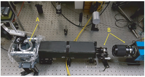
Figure 1.
FFD-PAT setup developed in Graz. The sample to be imaged is mounted and rotated on stage A. Full field projections of are recorded with the CCD camera B using an optical phase contrast technique. For a detailed description of the working principle, see the original works [30,31].
In this paper, for the first time, we study image reconstruction in FFD-PAT with a spatially variable speed of sound. We will give a precise mathematical formulation of FFD-PAT and describe the inverse problem we are dealing with (see Section 2). For its solution, we propose a two-step process. In the first step, the acoustic pressure at time T is reconstructed pointwise from the FFD data. In the second step, we recover the desired initial pressure distribution from the known valued of the pressure at time T. The first step can be approximated by inverting the well-known Radon transform. The second step consists in a final time wave inversion problem with spatially varying speed of sound. To the best of our knowledge, the latter has not been addressed in the literature so far. We develop iterative reconstruction methods based on an explicit computation of an adjoint problem. As main theoretical results of this paper, we establish uniqueness and stability of the final time wave inversion problem (see Section 3). In particular, this implies linear convergence for the proposed iterative reconstruction methods. In Section 4, we present numerical results demonstrating that the proposed algorithm is efficient and stable. Moreover, the presented numerical results clearly highlight the importance of taking sound speed variations into account in FFD-PAT image reconstruction.
2. Full Field Detection Photoacoustic Tomography
In this section, we describe a mathematical model for FFD-PAT including the variable sound speed case, and state the inverse problem under consideration. Additionally, we outline the proposed two-step reconstruction procedure and formulate the final time inverse problem.
2.1. Mathematical Model
In the case of variable sound speed, acoustic wave propagation in PAT is commonly described by the initial value problem [34,38,39,41]
here is the sound speed at location and is the initial pressure distribution that encodes the inner structure of the object. It is assumed that the object is contained inside the ball , of radius R centered at the origin, and that the sound speed is smooth, positive and has the constant value outside . We denote by the set of all smooth functions that vanish outside .
In FFD-PAT, linear projections (integrals along straight lines) of the 3D pressure field for a fixed time are recorded. As illustrated in Figure 1, this can be implemented using a special phase contrast method and a CCD-camera that records full field projections of the pressure field [30,31]. The linear projections are collected for rotation angles around the axis and are given by
for . Here determines the set of admissible projections and the defining condition means that in practice only pressure integrals over those lines are recorded, which do not intersect the possible support of the imaged object; compare Figure 2.

Figure 2.
Horizontal cross-section of the FFD-PAT setup.. Full field projections are measured over lines that do not intersect the ball . Consequently, for any plane , integrals of over those lines are given that do not intersect the disc . For planes with , this yields the exterior problem for the Radon transform.
2.2. Description of the Inverse Problem
In order to describe the inverse problem of FFD-PAT in a compact way, we introduce some further notation. First, we define the operator
where p denotes the solution of (1)–(3). The operator maps the initial data f to the solution (full field) of the wave Equations (1)–(3) at the given measurement time . Second, we define the X-ray transform
Note that for any fixed , the function is the Radon transform of in the horizontal plane . Finally, we define the restricted X-ray transform
For , is the exterior Radon transform of and consist of integrals over lines not intersecting the disc ; compare Figure 2. Otherwise, coincides with the standard Radon transform of .
Using the operator notation introduced above we can write the inverse problem of FFD-PAT in the form
Evaluation of is referred to as the forward problem in FFD-PAT. In this paper, we study the solution of the inverse problem (8).
2.3. Two-Step Reconstruction
One possible approach to solve the inverse problem of FFD-PAT is to directly recover f from data in (8) via iterative methods. Typically, each iteration step requires the evaluation of the forward operator and its adjoint . In this paper, we consider a two-step approach where we first invert via a direct method and then use an iterative method to invert . This avoids repeated and time consuming evaluation of and its adjoint. The proposed reconstruction method consists of the following two steps.
- ■
- Inverse Radon transform: Assume that projection data are given and consider the zero extension by for and otherwise. We then define an approximation to by applying an inversion formula of the Radon transform in planes . Using the well-known filtered backprojection inversion formula for the Radon transform [42] yieldswhere denotes the principal value integral.
- ■
- Final time wave inversion: For the second step, assume that an approximation to the 3D acoustic field at time T is given. Recovering the initial pressure then yields the final time wave inversion problemTo the best of our knowledge, the final time wave inversion problem (9) has not been considered so far and its investigation will be the main theoretical focus of this work.
For solving the wave inversion problem (9), we propose iterative solution methods that are described in Section 3. As main theoretical results, we derive its uniqueness and stability.
Another possible approach for solving the first step would be to work with the exterior Radon transform [43,44,45]. Instead, we invert the standard Radon transform after setting the missing values of to zero. We observe numerically that the missing values are indeed close to zero for large enough measurement time T. Although we do not have a rigorous mathematical proof for this claim, it is supported by at least two facts. First, in the case of a non-trapping sound speed, the known decay estimate [46] for the solution p of (1)–(3) with initial data f supported in states
for all . Here is a constant only depending on and T, and is a constant depending on . Second, in the case of constant sound speed, the X-ray transform reduces (1)–(3) to a 2D wave equation with initial data supported in a disc of radius R. Thus, in the constant sound speed case, describes 2D propagation which rapidly decays inside the disc. Formulating and proving precise statements in such a direction, however, is an interesting unsolved problem.
3. Final Time Wave Inversion Problem for Variable Sound Speed
In this section we study the final time wave inversion problem (9), where the forward operator is defined by (5). According to standard results for the wave equation [47], the forward operator extends to a bounded linear operator . Below we establish uniqueness and stability results and derive an iterative reconstruction algorithm. Note that for constant sound speed, recovering the function f from the solution at time T of (1) with initial data instead of , is equivalent to the inversion from spherical means with fixed radius. Uniqueness and an inversion method for this problem has been obtained in the classical book of Fritz John [48]. However, neither for the case of initial data nor in the variable sound speed case we are aware of any similar results.
3.1. Uniqueness and Stability Theorem
The following theorem is the main theoretical result of this paper and states that the final time wave inversion problem (9) has a unique solution that stably depends on the right-hand side.
Theorem 1 (Uniqueness and stability of inverting WT).
For a non-trapping speed of sound, the operator is injective and bounded from below.
The proof of Theorem 1 is presented in the following Section 3.2. See [19,41,49] for related results and methods in the case of standard PAT data. Theorem 1 states that
In particular, has a bounded inverse, where denotes the range of . The latter implies that gradient based iterative methods for (9) converge linearly, similar to the case of standard PAT data; see [38].
3.2. Proof of Theorem 1
Let c be a non-trapping sound speed. We first prove two crucial Lemmas, from which Theorem 1 follows rather quickly.
Lemma 1.
Assume that , then . That is, is injective.
Proof.
Let p denote the solution of (1)–(3). We will construct a solution of the wave equation which is periodic in time with period such that on . Once this is done, we obtain for any n. Using (10), we arrive at
It remains to construct the above-mentioned solution of the wave equation. The idea is to properly reflect the solution p in the time variable t through the time moments as follows. We first construct on by the odd reflection of p through the moment : for and for all . Since on , we obtain that and are continuous at . Therefore, p is continuous on and solves the wave equation on that interval. Next note that on . By the even reflection through : for all , we obtain that is a solution of the wave equation in . Finally, we extend the solution by periodicity with period . Noting that and , we obtain that and are continuous for all time and satisfies the wave equation in . This finishes our proof. □
Lemma 2.
There is a constant C and a pseudo-differential operator of order at most such that
Proof.
Let p denote the solution of wave Equations (1)–(3) and recall the parametrix formula ; see [47]. Here, the phase function solves the eikonal equation for with the initial condition . The amplitude function is a classical symbol , where is homogeneous of order in . Its leading term satisfies the transport equation
with the initial condition , see [41]. Here, only depends on the sound speed c and the phase function . Let us denote by the unit speed geodesics originating at along the direction . Then, is a characteristics curve of the above transport equation; that is, (12) reduces to a homogeneous ODE on each geodesic curve.
We then write
Each operator is a Fourier integral operator (FIO) with the canonical relation given by the pairs for any , unit vectors, , and . Let be equipped with the metrics . Then, is obtained by translating on the geodesic by the distance T. From the initial condition of and we see that, up to lower order terms,
Heuristically, under Equations (1)–(3), each singularity of f at is broken into two equal parts. They propagate along the geodesic in the opposite directions to generate a singularity of at .
From the standard theory of FIOs (see [50]), the adjoint translates back to and is a pseudo differential operator. On the other hand, is a FIO whose canonical relation consists of the pairs given by , and . That is, is an infinitely smoothing operator on B. Therefore, microlocally, we can write We will show that the principal symbol of satisfies . This result can be intuitively understood as follows. Let us consider and a singularity of f at . Under Equations (1)–(3), half of this singularity propagates into the direction (corresponding to the function ). At the moment , it is transformed to a singularity of at . Under the adjoint Equation (15), half of this singularity propagates back to at to generate a singularity of . It is natural to believe that this recovered singularity is of the original singularity of f (due to twice splitting, as described). The proof below verifies this intuition.
Indeed, denote by the solution of the time-reversed wave equation, e.g., Equation (15), with the initial condition given by . Then, by definition (see Theorem 2) . The solution can be decomposed into the sum . Here, , up to smooth terms, are solutions of the wave equations in and satisfy , . We are only concerned with since it defines . We can write
Let be the principal part of b. Then, the principal symbol of is given by . We note that satisfies the same equation as (see (12)). Therefore, on each bicharacteristic curve the ratio is constant which implies . Similar to the argument below Equation (13), up to lower order terms, we have
This and Equation (14) implies that . Therefore, we obtain . Combining with a similar argument for , we obtain that the principal symbol of is . That is, , where is a pseudodifferential operator of order at most and is the identity. We have and therefore conclude . □
We are now ready to prove Theorem 1.
Proof of Theorem 1.
Recall from Lemma 2 that where is a pseudo-differential operator of order at most . Since is compact and is injective, applying ([51] Theorem V.3.1), we obtain for some constant . This finishes our proof. □
3.3. Continuous Adjoint Operator
Iterative methods for solving (9) require knowledge of the adjoint operator of . In this subsection, we compute the continuous adjoint operator and prove that it is again given by the solution of a wave equation. More precisely, we have the following result.
Theorem 2.
Let , consider the time reversed final state problem for the wave equation,
and let denote the indicator function of . Then, .
Proof.
It is clearly sufficient to show , where u solves the wave equation on , with the final state conditions . Using the weak formulation (similar to [38]) for the wave equation, shows that for . Two times integration by parts, rearranging terms and using the final state conditions for u yields . By taking v as the solution of (1)–(3) this yields , which implies and completes the proof. □
We can reformulate the adjoint operator as follows.
Corollary 1.
For , let q be the solution of
with initial conditions . Then, .
3.4. Application of the Steepest 6hhod
We propose solving the finite time wave inversion problem (9) via gradient type methods applied to residual functional . Using standard PAT data, various iterative methods for PAT accounting for variable sound speed have been investigated in [36,37,38,39,40]. In particular, in [40] the steepest descent method has been demonstrated to be numerically efficient and robust. For the results shown in this paper we will therefore use the steepest-descent method. Our numerical experiments confirm that the steepest-descent method is also efficient for FFD-PAT and the final time wave inversion problem, where it reads as follows.
Because of the injectivity and boundedness of , the sequence of iterates generated by Algorithm 1 converges to the unique solution of (9). The stability result (11) even implies that the steepest descent method converges linearly for FFD-PAT. More precisely, the sequence generated by Algorithm 1 satisfies the estimate for some constant .
| Algorithm 1: Steepest descent method for solving . |
|
4. Numerical Simulations
In this section, we numerical present results using Algorithm 1 for FFD-PAT with variable sound speed. Recall that for constant speed of sound, reconstructions from experimental FFD-PAT data are shown in [30,31]. In the present study, we give numerical results for spatially varying speed of sound. Performing experimental measurements for samples with variable speed of sound and applying our algorithms to such data is subject of future research.
4.1. Discretization
To implement the steepest descent method (or other gradient type schemes), one has to discretize the final time wave operator and its adjoint . For that purpose we solve the forward and adjoint wave Equations (9) and (16) on a cubical grid with side length and nodes for with the k-space method [52,53], which we briefly recall in Appendix A. Note that the implementation of the k-space method yields a -periodic solution. The parameter L is chosen such that which implies that inside , for , the solution of (16) coincides with its -periodic extension.
We denote by the set of all with for . The discretized versions of and its adjoint are defined by and , respectively, where denotes the discretized wave propagation defined by the k-space method using the discrete time steps for , and is the discretized indicator function of the ball . The linear projection and its left inverse are implemented using the Matlab build in functions for the Radon and inverse Radon transforms, respectively, with equally spaced projection angles covering . The resulting discretized transforms are denoted by and , respectively.
4.2. Data Simulation
For the presented numerical results, we use , , , , and collect FFD-data for projection directions. As initial pressure we take the sum of three solid spheres, as show in the left picture in Figure 3. The used sound speed is shown in the right picture in Figure 3, and consist of two Gaussian peaks with opposite signs, added to the constant sound speed . The top row in Figure 4 shows the simulated FFD-PAT data (left) and the noisy FFD-PAT data (right) at projection angle for both cases. To generate the noisy FFD data we have added Gaussian white noise with a standard deviation of 10% of the maximal value of , resulting in a relative -data error %. For the first reconstruction step we apply the inverse Radon transform to the FFD-PAT data, resulting in the approximate 3D final time pressure . The reconstruction of final time pressure from noisy data is shown in the bottom right image in Figure 4. For comparison purpose, the simulated final time pressure is shown in the bottom left image in Figure 4.

Figure 3.
Phantom and sound speed used for the numerical simulations. (Left): Initial pressure (the phantom to be recovered). (Right): Spatially varying sound speed .
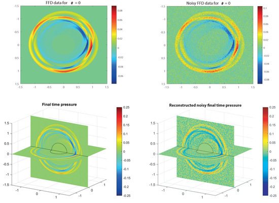
Figure 4.
FFD-PAT measurement data and final time pressure. (Top left): Simulated FFD-PAT data for projection direction . (Top right): Noisy FFD-PAT data for projection direction . (Bottom left): Simulated final time pressure . (Bottom right): Recovered final time pressure from noisy FFD-PAT data.
4.3. Reconstruction Results
To recover the initial pressure , we apply the steepest descent method (Algorithm 1) with to the point-wise approximation that is recovered in step one. Reconstruction results after 5 iterations are shown in Figure 5. The top row shows reconstruction results from simulated data and the middle row shows reconstruction results from noisy data, both using the correct sound speed for the reconstruction process. One observes, that the reconstruction results from simulated as well as from noisy data are quite accurate. This demonstrates that the proposed algorithm is efficient, accurate and stable with respect to noise. In both cases, the whole reconstruction procedure takes about 90 on a standard desktop PC.
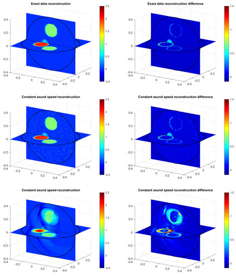
Figure 5.
Reconstructionsusing five iterations of the steepest descent algorithm (left) and the differencesto the true phantom (right). (Top): Using simulated data and correct sound speed . (Middle): Using noisy data and correct sound speed . (Bottom): Using simulated data data and wrong sound speed .
The bottom row in Figure 5 shows reconstruction results using the wrong constant sound speed in Algorithm 1 (while data generation still uses the inhomogeneous sound speed ). In this case, the reconstruction error is much larger, showing the relevance of integrating sound speed variations in image reconstruction. Finally, in Figure 6 we show reconstruction results with the previous Fourier method that has been derived in [31] under a constant sound speed assumption. The results with the Fourier method show a large reconstruction error and are very similar to the reconstruction result using the steepest descent method assuming constant sound speed. This demonstrates that the artifacts in both cases are due to the wrong wave propagation model, which further supports the importance of taking sound speed variations into account in FFD-PAT image reconstruction.

Figure 6.
Reconstruction(left) and the difference(right) using the Fourier algorithm. Note that the Fourier algorithm assumes constant sound speed in the image reconstruction, similar to the results shown in the bottom row of Figure 5.
4.4. Quantitative Error Analysis
For all results shown in Figure 5, we stopped the steepest decent method after five iterations, since the reconstructions did not significantly improve by using more iterations. In fact, even after a single iteration, the -reconstruction error and the -residual error are quite close to their minimal values. This phenomenon is investigated in a more quantitative manner in Figure 7. The images on the left-hand side show the evaluation of the relative -reconstruction error in dependence of the iteration index k. The images on the right show the relative residual errors . The rapid convergence of both error metrics indicates that the finite time inversion problem is well conditioned, which is also suggested by our theoretical analysis presented in Section 3. The relative data errors, residuals and reconstruction errors for all reconstructions shown above are summarized in Table 1.

Figure 7.
Relative reconstruction error (left) and relative residuals (right). (Top): Simulated data and correct sound speed. (Middle): Noisy data and correct sound speed. (Bottom): Simulated data and wrong sound speed (constant and equal to one).

Table 1.
Relative error metrics for the FFD data and reconstructions. The first column shows the relative -norm of the noise added to the data. The second column shows the relative -reconstruction error after step one (not applicable to Fourier reconstruction). The third column shows the relative residual error which are minimized in step 2 of the iterative algorithms. The last column shows the relative -error of final reconstruction.
5. Conclusions
In this paper, we investigated FFD-PAT, where projection data of acoustic pressure are measured. For the first time, the variable speed of sound has been taken into account for this kind of setup. We developed a two-step reconstruction procedure that recovers the 3D pressure in a first step, which is then used as input for a finite time wave inversion problem in a second step. As the main theoretical contribution of this paper we prove uniqueness and stability results for the finite time wave inversion problem. For the actual solution, we propose the steepest descent iteration which we found to be numerically efficient and stable for FFD-PAT. Moreover, our numerical results demonstrate that ignoring sound speed variations significantly degrades the reconstruction quality. We point out that the novelties of the paper are the development of a reconstruction method together with a mathematical uniqueness and stability analysis of the arising final time wave inversion problem for FFD-PAT with variable sound speed. The experimental feasibility of FFD-PAT has been demonstrated previously in [30,31]. In future work we will perform experiments using FFD-PAT with spatially variable sound speed and experimentally verify our two-step algorithm. Moreover, in upcoming work we will study limited view problems for FFD-PAT which naturally arise in applications, for instance in the case of breast imaging.
Author Contributions
M.H. and G.Z. developed the reconstruction algorithms, the numerical implementation and performed the numerical experiments; L.N. established the uniqueness and stability results; M.H., G.Z., L.N. and R.N. wrote the paper; M.H. and R.N. supervised the project.
Funding
G.Z. and M.H. acknowledge support of the Austrian Science Fund (FWF), project P 30747-N32. The research of L.N. is supported by the National Science Foundation (NSF) Grants DMS 1212125 and DMS 1616904. The work of R.N. has been supported by the FWF, project P 28032.
Conflicts of Interest
The authors declare no conflicts of interest.
Appendix A. k-Space Method
We briefly describe the k-space method for the 3D wave Equations (1)–(3) as we use it for the numerical computation of and . The k-space method is an attractive alternative to standard methods using finite differences, finite elements or pseudospectral methods, since it does not suffer from numerical dispersion [52,53]. It utilizes the decomposition , where are defined by and where denotes maximal speed of sound. It can be checked that with this definition of v and w the wave equation with variable speed of sound splits into the system and . In the k-space method we use the time stepping formula
where and denote the Fourier transform and its inverse with respect to space and frequency variables and and is the time step size. This equivalent formulation motivates the following algorithm for numerically solving the wave equation.
| Algorithm A1: k-space method for numerically solving (1)–(3). |
|
References
- Beard, P. Biomedical photoacoustic imaging. Interface Focus 2011, 1, 602–631. [Google Scholar] [CrossRef] [PubMed]
- Kruger, R.A.; Kopecky, K.K.; Aisen, A.M.; Reinecke, R.D.; Kruger, G.A.; Kiser, W.L. Thermoacoustic CT with Radio waves: A medical imaging paradigm. Radiology 1999, 200, 275–278. [Google Scholar] [CrossRef] [PubMed]
- Wang, L.V. Multiscale photoacoustic microscopy and computed tomography. Nat. Photonics 2009, 3, 503–509. [Google Scholar] [CrossRef]
- Wang, K.; Anastasio, M. Photoacoustic and thermoacoustic tomography: Image formation principles. In Handbook of Mathematical Methods in Imaging; Springer: Berlin, Germany, 2011; pp. 781–815. [Google Scholar]
- Xu, M.; Wang, L.V. Photoacoustic imaging in biomedicine. Rev. Sci. Instrum. 2006, 77, 041101. [Google Scholar] [CrossRef]
- Agranovsky, M.; Kuchment, P.; Kunyansky, L. On reconstruction formulas and algorithms for the thermoacoustic tomography. In Photoacoustic Imaging and Spectroscopy; Wang, L.V., Ed.; CRC Press: Boca Raton, FL, USA, 2009; pp. 89–101. [Google Scholar]
- Filbir, F.; Kunis, S.; Seyfried, R. Effective discretization of direct reconstruction schemes for photoacoustic imaging in spherical geometries. SIAM J. Numer. Anal. 2014, 52, 2722–2742. [Google Scholar] [CrossRef]
- Finch, D. The spherical mean value operator with centers on a sphere. Inverse Probl. 2007, 23, 37–49. [Google Scholar] [CrossRef]
- Finch, D.; Haltmeier, M. Rakesh Inversion of spherical means and the wave equation in even dimensions. SIAM J. Appl. Math. 2007, 68, 392–412. [Google Scholar] [CrossRef]
- Finch, D.; Patch, S.K. Determining a function from its mean values over a family of spheres. SIAM J. Math. Anal. 2004, 35, 1213–1240. [Google Scholar] [CrossRef]
- Haltmeier, M. Universal inversion formulas for recovering a function from spherical means. SIAM J. Math. Anal. 2014, 46, 214–232. [Google Scholar] [CrossRef]
- Haltmeier, M. Exact Reconstruction Formula for the Spherical Mean Radon Transform on Ellipsoids. Inverse Probl. 2014, 30, 035001. [Google Scholar] [CrossRef]
- Haltmeier, M.; Pereverzyev, S., Jr. The universal back-projection formula for spherical means and the wave equation on certain quadric hypersurfaces. J. Math. Anal. Appl. 2015, 429, 366–382. [Google Scholar] [CrossRef]
- Haltmeier, M.; Schuster, T.; Scherzer, O. Filtered backprojection for thermoacoustic computed tomography in spherical geometry. Math. Methods Appl. Sci. 2005, 28, 1919–1937. [Google Scholar] [CrossRef]
- Kuchment, P.; Kunyansky, L.A. Mathematics of thermoacoustic and photoacoustic tomography. Eur. J. Appl. Math. 2008, 19, 191–224. [Google Scholar] [CrossRef]
- Kunyansky, L.A. Explicit inversion formulae for the spherical mean Radon transform. Inverse Probl. 2007, 23, 373–383. [Google Scholar] [CrossRef]
- Kunyansky, L.A. A series solution and a fast algorithm for the inversion of the spherical mean Radon transform. Inverse Probl. 2007, 23, S11–S20. [Google Scholar] [CrossRef]
- Natterer, F. Photo-acoustic inversion in convex domains. Inverse Probl. Imaging 2012, 6, 315–320. [Google Scholar] [CrossRef]
- Nguyen, L.V. A family of inversion formulas for thermoacoustic tomography. Inverse Probl. Imaging 2009, 3, 649–675. [Google Scholar] [CrossRef]
- Xu, M.; Wang, L.V. Universal back-projection algorithm for photoacoustic computed tomography. Phys. Rev. E 2005, 71, 016706. [Google Scholar] [CrossRef] [PubMed]
- Haltmeier, M.; Zangerl, G. Spatial resolution in photoacoustic tomography: Effects of detector size and detector bandwidth. Inverse Probl. 2010, 26, 125002. [Google Scholar] [CrossRef]
- Roitner, H.; Haltmeier, M.; Nuster, R.; O’Leary, D.P.; Berer, T.; Paltauf, G.; Grün, H.; Burgholzer, P. Deblurring algorithms accounting for the finite detector size in photoacoustic tomography. J. Biomed. Opt. 2014, 19, 056011. [Google Scholar] [CrossRef] [PubMed]
- Rosenthal, A.; Ntziachristos, V.; Razansky, D. Model-based optoacoustic inversion with arbitrary-shape detectors. Med. Phys. 2011, 38, 4285–4295. [Google Scholar] [CrossRef]
- Wang, L.V. An imaging model incorporating ultrasonic transducer properties for three-dimensional optoacoustic tomography. IEEE Trans. Med. Imaging 2011, 30, 203–214. [Google Scholar] [CrossRef] [PubMed]
- Burgholzer, P.; Hofer, C.; Paltauf, G.; Haltmeier, M.; Scherzer, O. Thermoacoustic tomography with integrating area and line detectors. IEEE Trans. Ultrason. Ferroelectr. Freq. Control 2005, 52, 1577–1583. [Google Scholar] [CrossRef] [PubMed]
- Burgholzer, P.; Bauer-Marschallinger, J.; Grün, H.; Haltmeier, M.; Paltauf, G. Temporal back-projection algorithms for photoacoustic tomography with integrating line detectors. Inverse Probl. 2007, 23, S65–S80. [Google Scholar] [CrossRef]
- Haltmeier, M.; Scherzer, O.; Burgholzer, P.; Paltauf, G. Thermoacoustic computed tomography with large planar receivers. Inverse Probl. 2004, 20, 1663. [Google Scholar] [CrossRef]
- Paltauf, G.; Nuster, R.; Haltmeier, M. Experimental evaluation of reconstruction algorithms for limited view photoacoustic tomography with line detectors. Inverse Probl. 2007, 23, S81–S94. [Google Scholar] [CrossRef]
- Zangerl, G.; Scherzer, O.; Haltmeier, M. Exact series reconstruction in photoacoustic tomography with circular integrating detectors. Commun. Math. Sci. 2009, 7, 665–678. [Google Scholar]
- Nuster, R.; Zangerl, G.; Haltmeier, M.; Paltauf, G. Full field detection in photoacoustic tomography. Opt. Express 2010, 18, 6288–6299. [Google Scholar] [CrossRef]
- Nuster, R.; Slezak, P.; Paltauf, G. High resolution three-dimensional photoacoustic tomography with CCD-camera based ultrasound detection. Biomed. Opt. Express 2014, 5, 2635–2647. [Google Scholar] [CrossRef]
- Niederhauser, J.J.; Weber, D.F.H.P.; Frenz, M. Real-time optoacoustic imaging using a Schlieren transducer. Appl. Phys. Lett. 2002, 81, 571–573. [Google Scholar] [CrossRef]
- Niederhauser, J.J.; Jäger, M.; Frenz, M. Real-time three-dimensional optoacoustic imaging using an acoustic lens system. Appl. Phys. Lett. 2004, 85, 846–848. [Google Scholar] [CrossRef]
- Jin, X.; Wang, L.V. Thermoacoustic tomography with correction for acoustic speed variations. Phys. Med. Biol. 2006, 51, 6437. [Google Scholar] [CrossRef] [PubMed]
- Ku, G.; Fornage, B.D.; Xing, J.; Xu, M.; Hunt, K.K.; Wang, L.V. Thermoacoustic and photoacoustic tomography of thick biological tissues toward breast imaging. Med. Phys. 1995, 22, 1605–1609. [Google Scholar] [CrossRef] [PubMed]
- Belhachmi, Z.; Glatz, T.; Scherzer, O. A direct method for photoacoustic tomography with inhomogeneous sound speed. Inverse Probl. 2016, 32, 045005. [Google Scholar] [CrossRef]
- Arridge, S.R.; Betcke, M.M.; Cox, B.T.; Lucka, F.; Treeby, B.E. On the adjoint operator in photoacoustic tomography. Inverse Probl. 2016, 32, 115012. [Google Scholar] [CrossRef]
- Haltmeier, M.; Nguyen, L.V. Analysis of Iterative Methods in Photoacoustic Tomography with variable Sound Speed. SIAM J. Imaging Sci. 2017, 19, 751–781. [Google Scholar] [CrossRef]
- Huang, C.; Wang, K.; Nie, L.; Wang, L.V.; Anastasio, M.A. Full-wave iterative image reconstruction in photoacoustic tomography with acoustically inhomogeneous media. IEEE Trans. Med. Imaging 2013, 32, 1097–1110. [Google Scholar] [CrossRef] [PubMed]
- Nguyen, L.V.; Haltmeier, M. Reconstruction algorithms for photoacoustic tomography in heterogenous damping media. arXiv, 2018; arXiv:1808.06176v1. [Google Scholar]
- Stefanov, P.; Uhlmann, G. Thermoacoustic tomography with variable sound speed. Inverse Probl. 2009, 25, 075011. [Google Scholar] [CrossRef]
- Natterer, F. The Mathematics of Computerized Tomography; SIAM: Philadelphia, PA, USA, 1986. [Google Scholar]
- Kuchment, P. The Radon Transform and Medical Imaging; SIAM: Philadelphia, PA, USA, 2014; Volume 85. [Google Scholar]
- Quinto, E. Singular value decompositions and inversion methods for the exterior Radon transform and a spherical transform. J. Math. Anal. Appl. 1983, 95, 437–448. [Google Scholar] [CrossRef][Green Version]
- Quinto, E. Tomographic reconstructions from incomplete data-numerical inversion of the exterior Radon transform. Inverse Probl. 1988, 4, 867. [Google Scholar] [CrossRef]
- Vainberg, B. On the short wave asymptotic behaviour of solutions of stationary problems and the asymptotic behaviour as t→∞ of solutions of non-stationary problems. Rus. Math. Surv. 1975, 30, 1–58. [Google Scholar] [CrossRef]
- Tréves, F. Introduction to Pseudodifferential and Fourier Integral Operators Volume 2: Fourier Integral Operators; Springer Science & Business Media: Berlin, Germany, 1980. [Google Scholar]
- John, F. Partial Differential Equations. In Applied Mathematical Sciences, 4th ed.; Springer: New York, NY, USA, 1982; Volume 1. [Google Scholar]
- Nguyen, L.V. On singularities and instability of reconstruction in thermoacoustic tomography. Tomogr. Inverse Transp. Theory Contemp. Math. 2011, 559, 163–170. [Google Scholar]
- Hörmander, L. Fourier integral operators. I. Acta Math. 1971, 127, 79–183. [Google Scholar] [CrossRef]
- Taylor, M.E. Pseudodifferential Operators, Volume 34 of Princeton Mathematical Series; Princeton University Press: Princeton, NJ, USA; Springer Science & Business Media: Berlin, Germany, 1981. [Google Scholar]
- Cox, B.T.; Kara, S.; Arridge, S.R.; Beard, P.C. k-space propagation models for acoustically heterogeneous media: Application to biomedical photoacoustics. J. Acoust. Soc. Am. 2007, 121, 3453–3464. [Google Scholar] [CrossRef]
- Mast, T.D.; Souriau, L.P.; Liu, D.L.; Tabei, M.; Nachman, A.I.; Waag, R.C. A k-space method for large-scale models of wave propagation in tissue. IEEE Trans. Ultrason. Ferroelectr. Freq. Control 2002, 48, 341–354. [Google Scholar] [CrossRef]
© 2019 by the authors. Licensee MDPI, Basel, Switzerland. This article is an open access article distributed under the terms and conditions of the Creative Commons Attribution (CC BY) license (http://creativecommons.org/licenses/by/4.0/).