A Trimmed Clustering-Based l₁-Principal Component Analysis Model for Image Classification and Clustering Problems with Outliers

Abstract

Different versions of principal component analysis (PCA) have been widely used to extract important information for image recognition and image clustering problems. However, owing to the presence of outliers, this remains challenging. This paper proposes a new PCA methodology based on a novel discovery that the widely used $l_1$-PCA is equivalent to a two-groups $k$-means clustering model. The projection vector of the $l_1$-PCA is the vector difference between the two cluster centers estimated by the clustering model. In theory, this vector difference provides inter-cluster information, which is beneficial for distinguishing data objects from different classes. However, the performance of $l_1$-PCA is not comparable with the state-of-the-art methods. This is because the $l_1$-PCA can be sensitive to outliers, as the equivalent clustering model is not robust to outliers. To overcome this limitation, we introduce a trimming function to the clustering model and propose a trimmed-clustering based $l_1$-PCA (TC-PCA). With this trimming set formulation, the TC-PCA is not sensitive to outliers. Besides, we mathematically prove the convergence of the proposed algorithm. Experimental results on image classification and clustering indicate that our proposed method outperforms the current state-of-the-art methods.

1. Introduction

Image classification and clustering problems are topics fundamental to various areas of machine learning [1,2,3] including image recognition and image clustering. Principal component analysis (PCA) has been widely used to perform dimensionality reduction and extract useful information for these problems [4,5,6,7,8,9,10,11]. One of the common objectives of dimensionality reduction is to retain the most important information that is beneficial to data processing tasks and meanwhile filter out corrupted and noisy information from the dataset. One example is the face recognition problem. A face database may contain face images with occlusions such as scarves, sunglasses and so forth. Obviously, the key information that can recognize a person is the facial features not the scarves nor the sunglasses. A good dimension reduction method can effectively extract the key facial features and, at the same time, ignore the occluded information. Another example is the image clustering problem. The purpose of clustering is to partition the data into different clusters and group the similar data objects together. However, similar to the above face recognition problem, the corrupted and noisy information such as scarves can make two facial images very different even they are taken from the same person. This makes the clustering task very challenging. Again, a good dimension reduction method can filter out the scares and retain the key facial features and gives a more accurate clustering result.

The major challenge of PCA for supervised classification and unsupervised clustering problems is how to extract important information that can distinguish the characteristics of different classes/clusters from a corrupted and noisy dataset. For a face recognition problem, the facial features of different persons are the key to distinguish them. However, the corrupted and noisy information can be a factor that cause the difference among different facial images. Figure 1 shows two frontal face images and two facial images with scares. Obviously, facial features such as eyes of these persons are a bit different. They can be used to distinguish these persons. However, the face with scarves and the face without scarves are different. Also, the two scarves are different too. If the dimension reduction method wrongly identifies the scarves as the key features that cause the difference, the accuracy of the trained recognition system may heavily depend on this occluded information and lead to a poor recognition result. In image recognition and clustering problem, this kind of data object is known as outlier. This means the data object carry corrupted and noisy information.

Many different methods have been proposed to solve the above outlier problem. However, these techniques still have evident defects when applied to real-world classification and clustering problems. The very first method used to extract the important information of the data is to apply eigenvalue decomposition to the covariance matrix of the data [12]. The eigenvectors with small eigenvalues are discarded and the eigenvectors with large eigenvalues are retained for classification or clustering. This method works well only if the data do not contain any outlier. This is because an eigenvector of a covariance matrix represents the variance of the data in a specific direction. However, the occlusion of a facial image can cause large variation as well. The eigenvectors with large eigenvalues can wrongly identify the occluded information as important information. To address this problem, different $l_p$ norm-based methods have been proposed. One example is the $l_1$-PCA, which adopts the $l_1$ norm to measure the variation of features of the data [13,14]. This approach replaces the squared $l_2$ norm that is adopted by the classical PCA by a $l_1$ norm. The $l_1$ norm measure usually gives a much lower weight to the data objects that are far away from the majority. Although this approach is proved to be more robust to outliers and more effective than the classical PCA, seldom work is devoted to study how this approach extract information that can distinguish different classes or clusters for the classification or clustering problems. Another popular approach is the rank-based PCA method. Its idea is to decompose the data matrix into a single low-rank matrix and a sparse component [15,16,17]. The low-rank matrix approximates the common features that are linearly correlated in the data while the sparse component approximates less frequently appeared features and these are assumed to be the corrupted and noisy information. For face recognition or clustering problem, the low-rank matrix represents the common facial features of different images that are highly correlated to each other. The scarves and sunglasses are less frequently appeared features in the database. They are relatively sparse information and belong to the sparse component. Although this approach can effectively identify the occluded information, it may discard some information that can distinguish the characteristics of different classes or clusters. In the low-rank formulation, the common facial features of different data objects are not strictly linearly correlated to each other. Some people may have larger eyes while some may have more attractive lips. These are key characteristics to distinguish different people. However, these are less frequently appeared features. They may be discarded and treated as sparse information.

To alleviate the aforementioned issues, we introduce a modified version of the $l_1$-PCA, which incorporates clustering with $l_1$-PCA. We find that the superiority performance of the $l_1$-PCA over the classical PCA is not only because of the $l_1$ norm formulation but also its ability to extract information that is beneficial to image classification and clustering problems. We mathematically prove that the $l_1$-PCA can be expressed as a special two-group $k$-means clustering problem. The projection vector of the $l_1$-PCA is the vector difference between the two cluster centers obtained by the $k$-means clustering problem. If the two clusters are two different classes of the data, the corresponding vector difference represents the inter-class direction that groups data objects with similar nature together. This is beneficial to distinguish the two classes. Figure 2 illustrates this situation. This figure shows two classes of data. The left cluster forms a class while the right cluster forms another class. The red stars are the cluster centers of the two different classes. The vector difference between these two centers is in the horizontal direction. Apparently, the horizontal direction provides the key information to distinguish the two classes. Although the $l_1$-PCA possesses this important property, its performance is not as good as the state-of-the-art methods. The reason is that the $k$-means clustering algorithm adopts the squared $l_2$ norm in the formulation and is not robust to outliers. In other words, the $l_1$-PCA is not robust to outlier. To overcome this limitation, we propose a new method, namely, trimmed-clustering based l₁-PCA (TC-PCA) that replaces the squared $l_2$ norm by a trimming function in the special $k$-means clustering algorithm. The contributions of this paper are as follows.

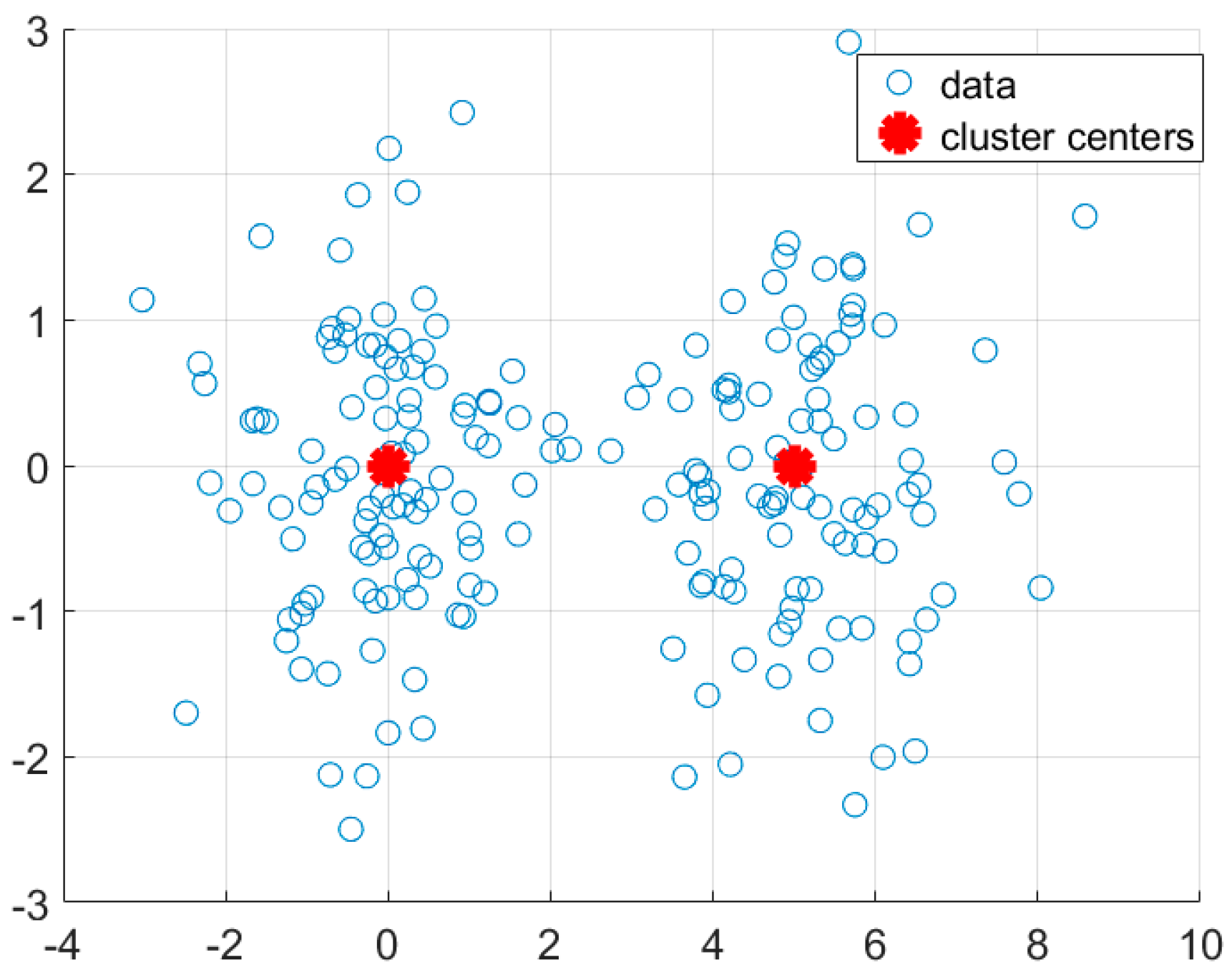
• We prove that the l₁-PCA is equivalent to a two-group k-means clustering model. The projection vector estimated by the $l_1$-PCA is the vector difference between the two cluster centers that are obtained by the $k$-means clustering algorithm. In other words, the projection vector of the $l_1$-PCA represents the inter-cluster direction, that is beneficial to distinguish data objects from different classes.
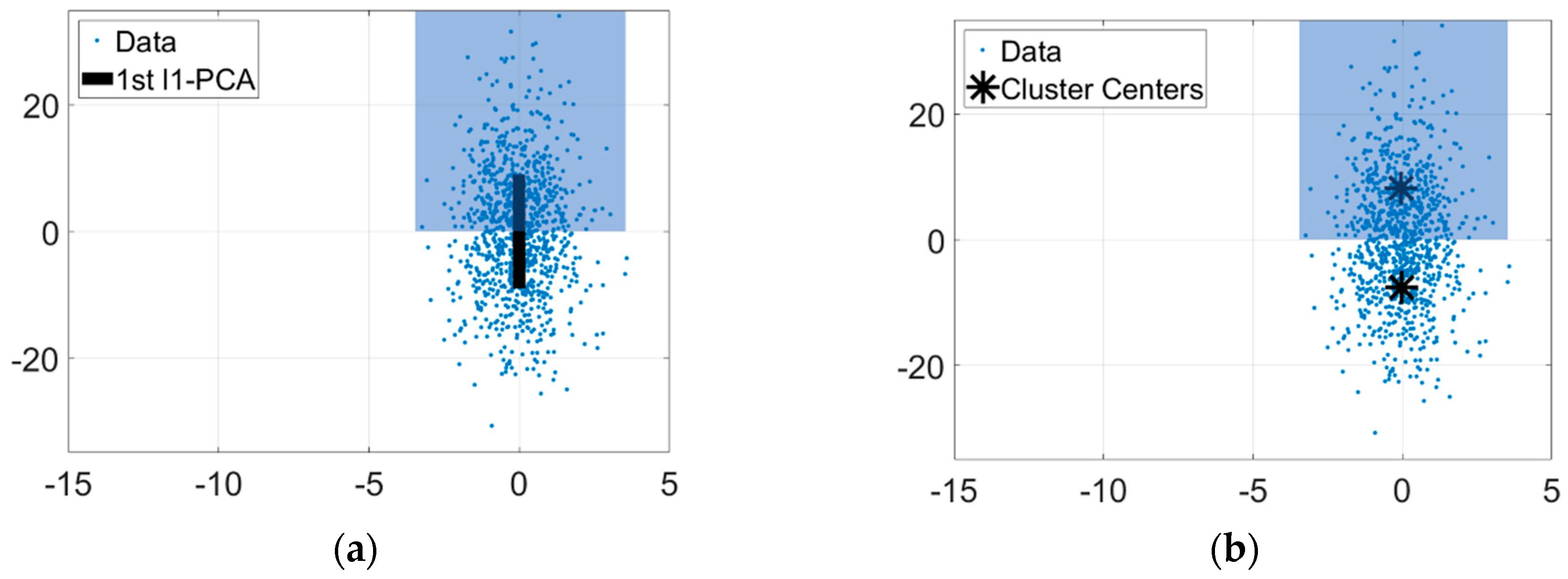
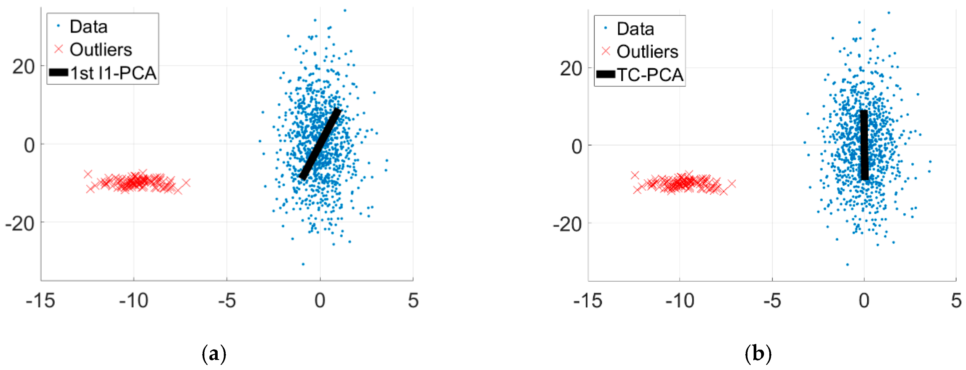
• We propose a novel TC-PCA model by integrating a trimming set into the two-group k-means clustering model, which makes the proposed method not sensitive to outliers.
• We mathematically prove that the estimator of TC-PCA is insensitive to outliers, which shows the robustness of the proposed method. In addition, we mathematically prove the convergence of the proposed algorithm.

This paper is organized as follows. In the next section, we briefly review related work. Section 3 presents the proposed TC-PCA model and the overall implementation. In addition, we discuss the mathematical properties and performance of the proposed method. Experimental results are shown in Section 4 and Section 5 concludes the paper.

2. Related Work

The current PCA methodologies typically adopt the following two ways to obtain projection vectors and they are the $l_p$ norm based estimator and the rank based estimator.

(i) $l_p$ norm based estimator: it models the projection vectors by a function of a $l_p$ norm. In contrast with the classical squared $l_2$ norm, the $l_p$ norm gives much smaller function values to the data objects that are far away from the majority. This can diminish the negative effect caused by outliers. One of the best known and most influential approaches is the l₁-PCA, which produces projection vectors by maximizing the l₁-norm of the projected data. However, owing to singularity of the $l_1$ norm, many different solvers have been proposed. In Reference [13], the l₁-PCA was reformulated as a linear programming problem, which was then solved by the simplex method. The authors in Reference [18] adopted a relaxation approach that turns the binary constraint into a semi-definite constraint and applied the interior point method to obtain the optimal solution. Kwak [14] reformulated the l₁-PCA and expressed the optimization problem by the composition constraints of l₁ and l₂-norms. This method finds one projection vector at a time. An orthogonalization procedure is incorporated to find the rest of the projection vectors. Later, the PCA with non-greedy l₁-norm maximization [19] was proposed. In contrast with the $l_1$-PCA, the non-greedy approach can find all required projection vectors at once. Zhou et al. [20] directly incorporated a $l_1$-norm penalty to the original PCA formulation, which performed feature selection for image classification and clustering problems. To find an optimal solution of the $l_1$-PCA in non-greedy form, Markopoulos et al. [21] proposed a polar expression to the data matrix and expressed the problem in a dual form. Their method can effectively search through all possibilities and output a very high-quality solution. Later, Markopoulos et al. [22] proposed a different solver based on bit-flipping iterations. Kwak [23] generalized l₁-PCA by replacing the $l_1$ norm by a general $l_p$ norm. More recently, Luo et al. [24,25] proposed a novel $l_{2,1}$-norm based PCA that does not require data centralization for dimensionality reduction. Variants of l₁-PCA have been proposed and they are formulated as a minimization of a residual function. In References [26] and [27], the authors introduced the $l_1$-norm residual function and adopted an alternative convex optimization together with divide-and-conquer approach, respectively, to find the projection vectors. Other than $l_1$ norm, Nie et al. [28] proposed the l₂-norm residual function with an optimal mean strategy to automatically obtain the center of the dataset. He et al. [29] proposed a residual function of squared $l_2$-norm to PCA algorithm based on maximum correntropy and solved by a half-quadratic optimization method. More recently, Nie et al. [30] proposed a more general $l_p$-norm based residual function named as $l_{2,p}$-norm PCA for image recognition problems. Other than the above PCA problems, $l_p$ norm based estimators are also widely used in other types of dimensionality approaches including 2DPCA, LDA, 2DLDA, tensor and so forth. Li et al. [31] applied the $l_1$-norm formulation for 2DPCA [1]. Ju et al. [32] introduced a probabilistic formulation for the $l_1$-norm based 2DPCA with the aid of variational inference. Other than 2DPCA, it is also widely applied in LDA. Zhong et al. [33] and Liu et al. [34] proposed the use of the $l_1$-norm in the LDA formulation. They replaced the squared $l_2$-norm for distance between classes and within classes by the $l_1$-norm. Wang et al. [35] introduced a non-greedy $l_1$-norm technique for the 2DLDA.

(ii) Rank-based estimator: its idea is to decompose the data matrix into a sparse matrix and a low-rank matrix, which is a polished version of the original dataset with low-rank feature. This approach generally assumes that all data objects are sparsely corrupted, and the key characteristics of the data can be represented by a low-rank matrix. In References [15,16,17], the authors proposed a robust PCA (RPCA) to recover the low-rank matrices via convex optimization. The idea of RPCA is to modify the entries of data matrix in the sense of l₁-norm so that the rank of matrix is minimized. The RPCA is widely used in various applications such as video surveillance [36], dictionary learning [37,38], compressed hyperspectral imaging and face recognition [39]. Zhang et al. [40] improved the RPCA by introducing another $l_1$-norm penalty that further regularizes the low-rank matrix. Sun et al. [32] enhanced the RPCA for video surveillance problem by introducing a local regularization term to the model that can better preserve the local structure of the image data. Wang et al. [41] proposed a probabilistic robust matrix factorization that formulated the sparse component with a Laplace prior and the two matrices for the low-rank component with a Gaussian prior. Wang et al. [42] improved the probabilistic robust matrix factorization model and proposed a new framework based on Bayesian formulation. They imposed conjugate priors (multivariate normal distribution and Wishart distribution) onto the low-rank component and a generalized inverse Gaussian distribution onto the sparse errors. Zhao et al. [43] modified the aforementioned Bayesian framework and introduced a two-level generative Gaussian approach to model the complex noise. Xue et al. [44] modified the RPCA by introducing a total variation and rank-1 constraints to the model.

3. A Trimmed-Clustering Based l₁-PCA Model

In this section, we show that the l₁-PCA is equivalent to the two-group k-means clustering model. We then mathematically prove the equivalence of these two models. After that, we present the proposed TC-PCA model and the algorithm to obtain a set of orthonormal projection vectors. Mathematical properties and performance of the proposed method will also be discussed.

3.1. Relating l₁-PCA to Two-Groups K-Means Clustering

Consider the following l₁-PCA

$$\underset{\Vert u{\Vert }_2=1}{max}{{\displaystyle \sum }}_{i=1}^n|{(x_i-c)}^{T}u|,$$

(1)

where u is the projection vector and c is a centroid of the dataset. The centroid $c$ is usually set as the mean or median of the whole data. In our proposed model, the projection vector $u$ can be obtained without necessity of data centralization procedure. This will be explained later. Now, we show that the $l_1$-PCA can be expressed as the two-group k-means clustering model below

$$J(\widehat{u},c,l)={{\displaystyle \sum }}_{i=1}^n(l_{i,1}{\Vert x_i-(\widehat{u}+c)\Vert }_2^2+l_{i,2}{\Vert x_i-(-\widehat{u}+c)\Vert }_2^2),$$

(2)

where ${\Vert \Vert }_2$ is the $l_2$ norm distance. $l=\left\{l_{i,1},l_{i,2}\right\}$ is the indicator variable with $l_{i,k}=1$, $k=1,2,$ if $x_i$ belongs to the $k\mathrm{th}$ cluster and 0 otherwise and $l_{i,2}=1-l_{i,1}$. This clustering model partitions the data to two disjoint parts. They are represented by the two centroids, $\widehat{u}+c$ and $-\widehat{u}+c$. The data points that are closer to $\widehat{u}+c$ are classified as first cluster and the rest are the second cluster. Now, we examine this property in $l_1$-PCA model. The absolute term of this model can be expressed as $|{(x_i-c)}^{T}u|=sign({(x_i-c)}^{T}u)({(x_i-c)}^{T}u)$. This expression introduces another interpretation of the $l_1$-PCA. The sign function virtually assigns $\left\{-1,1\right\}$ to each data point and each data point belongs to one of the two regions or $sign({(x_i-c)}^{T}u)=-1$. This assignment means that if the point $x_i-c$ is in the same semi-plane as $u$, it is assigned as the first cluster (i.e., $sign({(x_i-c)}^{T}u)=1$). Otherwise, it is the second cluster (i.e., $sign({(x_i-c)}^{T}u)=-1$). In other words, the point $x_i$ that is closer to $u+c$ belongs to the first cluster. If it is closer to $-u+c$, it belongs to the second cluster. This is the same as the two-group clustering model. Figure 3 gives a visual illustration to this relationship. Figure 3a shows the 1st projection vector obtained by the l₁-PCA on the 2-dimensional normal dataset with zero mean and variances 1 and 10, whereas Figure 3b shows the same dataset with the cluster centers estimated by the two-group k-means clustering model. In Figure 3a, the data points $x_i-c$ that are in the same semi-plane (${(x_i-c)}^{T}u>0$, the upper half of the data) of the vector $u$ belong to the first cluster (shaded region). Otherwise, they are in the opposite semi-plane (${(x_i-c)}^{T}u<0$, the lower half of the data) and belong to the second cluster (non-shaded region). In Figure 3b, the data are partitioned into two parts. The data points closer to the upper centroid belong to the first cluster (shaded region) while the rest of them belong to the second cluster (non-shaded region). With this connection, we can see that the vector difference between the two clusters (or $\widehat{u}+c-(-\widehat{u}+c)$) shown in Figure 3b is the projection vector $u$ shown in Figure 3a. This will be mathematically justified next.

The following gives a mathematical justification about the equivalence between the $l_1$-PCA model and the special two-group $k$-means clustering model. By expressing each absolute term as a binary variable $s_i$, Equation (1) becomes

$$\underset{\Vert u{\Vert }_2=1}{max}{\displaystyle \sum }_{i=1}^n|{(x_i-c)}^{T}u|=\underset{\Vert u{\Vert }_2=1}{max}\underset{s_i\in \left\{-1,1\right\}}{max}{\displaystyle \sum }_{i=1}^n{s}_i{(x_i-c)}^{T}u=\underset{s_i\in \left\{-1,1\right\}}{max}{\Vert {\displaystyle \sum }_{i=1}^n{s}_i(x_i-c)\Vert }_2.$$

(3)

The first equality holds because $|x|=\underset{s\in \left\{-1,1\right\}}{max}sx$. The second equality holds because $\underset{\Vert u{\Vert }_2=1}{max}{x}^{T}u=\Vert x{\Vert }_2$. It is noted that the maximum point of the $l_2$ norm function is the same as the squared $l_2$ norm function. That is,

$$\underset{s_i\in \left\{-1,1\right\}}{max}{\Vert {\displaystyle \sum }_{i=1}^n{s}_i(x_i-c)\Vert }_2\propto \underset{s_i\in \left\{-1,1\right\}}{max}{\Vert {\displaystyle \sum }_{i=1}^n{s}_i(x_i-c)\Vert }_2^2.$$

(4)

We will see that the variable $s_i$ in the $l_1$-PCA model is the difference of the two indicator variables of the $k$-means clustering algorithm. That is, $s_i=l_{i,1}-l_{i,2}$. The above squared $l_2$ norm function leads to the following binary quadratic programming problem:

$$\underset{s\in {\left\{-1,1\right\}}^n}{max}{s}^T{X_c}^T{X}_{c}s$$

(5)

where $X_c=\left[x_1-c,x_2-c,\dots ,x_n-c\right]$ and $s=\left[s_1,s_2,\dots ,s_n\right]\in {\mathbb{R}}^n$. Let $s_i=l_{i,1}-l_{i,2}\in \left\{-1,1\right\}$, $\widehat{u}=\lambda ·u$ with $\Vert u{\Vert }_2=1$ and $\lambda$ is a constant. The theoretical justification is complete if Equation (2) can be expressed as the above binary quadratic programming problem. It is noted that Equation (2) can be rewritten as

$$\begin{array}{l}J(\widehat{u},c,l)={\displaystyle {\displaystyle \sum }_{i=1}^n}(l_{i,1}{\Vert (x_i-c)-\widehat{u}\Vert }_2^2+l_{i,2}{\Vert (x_i-c)+\widehat{u}\Vert }_2^2)\\ ={\displaystyle {\displaystyle \sum }_{i=1}^n}(l_{i,1}({\Vert x_i-c\Vert }_2^2-2{(x_i-c)}^T\widehat{u}+{\lambda }^2)+l_{i,2}({\Vert x_i-c\Vert }_2^2+2{(x_i-c)}^T\widehat{u}+{\lambda }^2))\\ ={\displaystyle {\displaystyle \sum }_{i=1}^n}{\Vert |x_i-c|\Vert }_2^2-2\lambda {\displaystyle {\displaystyle \sum }_{i=1}^n}{s}_i({(x_i-c)}^{T}u)+n{\lambda }^2\end{array}$$

(6)

The second and third equality hold because ${\Vert \widehat{u}\Vert }_2^2={\lambda }^2$ and $\widehat{u}=\lambda ·u$. Thus,

$$J(\widehat{u},c,l)={\displaystyle \sum }_{i=1}^n{\Vert |x_i-c|\Vert }_2^2-2\lambda {\displaystyle \sum }_{i=1}^n{s}_i({(x_i-c)}^{T}u)+n{\lambda }^2$$

(7)

To minimize (7) with respect to $\lambda$, we need the following claim.

Claim: The global minimum value of the FUNCTION $f(x)=-2\gamma x+n{x}^2$ is $f(\gamma )=-\frac{{\gamma }^2}{n}$. Here, $\gamma$ and $n$ are constants. $n$ is a positive number.

Proof: $f^{\prime }(x)=2nx-2\gamma .f^{\prime }(x)=0\Rightarrow x=\gamma /n$,

$$f^{″}(x)=2n>0\Rightarrow x=\gamma /n is the global minimum.$$

By taking $\gamma =2{{\displaystyle \sum }}_{i=1}^n{s}_i({(x_i-c)}^{T}u)$ and $x=\lambda$ in the above claim, Equation (7) is written as

$$\begin{array}{l}\underset{\widehat{u},I}{min}J(\widehat{u},c,l)=\underset{s_i\in \left\{-1,1\right\}}{min}\underset{u}{min}\left({\displaystyle {\displaystyle \sum }_{i=1}^n}{\Vert |x_i-c|\Vert }_2^2-\frac{1}{n}{\left({\displaystyle {\displaystyle \sum }_{i=1}^n}{s}_i({(x_i-c)}^{T}u)\right)}^2\right)\\ =\underset{s_i\in \left\{-1,1\right\}}{min}\underset{u}{min}-\frac{1}{n}{\left({\displaystyle {\displaystyle \sum }_{i=1}^n}{s}_i({(x_i-c)}^{T}u)\right)}^2\\ =\underset{s_i\in \left\{-1,1\right\}}{min}-\frac{1}{n}{\Vert {\displaystyle {\displaystyle \sum }_{i=1}^n}{s}_i(x_i-c)\Vert }_2^2\\ =\underset{s\in {\left\{-1,1\right\}}^n}{min}-\frac{1}{n}{s}^T{X_c}^T{X}_{c}s\\ \propto \underset{s\in {\left\{-1,1\right\}}^n}{max}{s}^T{X_c}^T{X}_{c}s,\end{array}$$

which is equal to (5). The third equality holds because $\underset{\Vert u{\Vert }_2=1}{min}-x^{T}u=-\Vert x{\Vert }_2$. In other words, the l₁-PCA is essentially equivalent to the two-group k-means clustering model. This equivalence has three major implications. First, the projection vector $u$ estimated by the $l_1$-PCA is the normalized vector difference between the two cluster centers, $\widehat{u}+c$ and $\widehat{u}-c$, obtained by the clustering algorithm. That is, $u=\widehat{u}/{\Vert \widehat{u}\Vert }_2$. Second, the binary vector $s_i$ introduced in Equation (3) is the difference of the two indicator variables of the two-group k-means clustering model. Third, the projection vector $u$ can be obtained without data centralization procedure.

3.2. The Proposed Model

Based on the two-group k-means clustering model in (2), we propose the following trimmed-clustering based l₁-PCA (TC-PCA) model:

$$J_{obj}(v,l,\Omega (p))={\displaystyle \sum }_{x_i\in \Omega (p)}(l_{i,1}{\Vert x_i-v_1\Vert }_2^2+l_{i,2}{\Vert x_i-v_2\Vert }_2^2),$$

(8)

where $v=\left\{v_1,v_2\right\}$ is a set of cluster centers, $l=\left\{l_{i,1},l_{i,2}\right\}$ is the indicator variable with $l_{i,2}=1-l_{i,1}$ and

$$\Omega (p)=\{x_i:the first p\mathrm{th} percentile of l_{i,1}{\Vert x_i-v_1\Vert }_2^2+l_{i,2}{\Vert x_i-v_2\Vert }_2^2\}$$

(9)

is a trimming set containing samples that are close to the cluster centers. When $p=100$, all sample data will be considered whereas the trimming set is an empty set if $p=0$. A trimming set has been proved to be a robust M-estimator and has a high breakdown point property [45,46,47]. Following the parameter setting used in References [48] and [49], in this paper, we only consider 75% (i.e., $p=75$) of data to estimate the projection vectors.

Note that (8) is a special case of (2) by incorporating the trimming set into the two-group k-means clustering model and setting $c+\widehat{u}=v_1$ and $c-\widehat{u}=v_2$. Solving these two equations leads to

$$\widehat{u}=\frac{1}{2}(v_1-v_2)$$

(10)

3.3. The Overall Implementation

We shall provide the optimality conditions for (8) and present the overall implementation of the algorithm to estimate a collection of projection vectors.

Taking the first derivative of (8) with respect to $v_k$ and set it to zero, we obtain the optimality condition for $v_k$

$$0=\frac{\partial J_{obj}(v,l,\Omega (p))}{\partial v_k}={\displaystyle \sum }_{x_i\in \Omega (p)}{l}_{i,k}(v_k-x_i),k=1,2.$$

That is, we have

$$v_k=\frac{1}{{{\displaystyle \sum }}_{x_i\in \Omega (p)}{l}_{i,k}}{{\displaystyle \sum }}_{x_i\in \Omega (p)}{l}_{i,k}{x}_i,k=1,2,$$

(11)

which is the average of sample data in both the trimming set and the $k\mathrm{th}$ cluster. The optimality conditions for the indicator variables are

$$\begin{array}{c}{l}_{i,1}=\{\begin{array}{cc}1,& if {\Vert x_i-v_1\Vert }_2^2\le {\Vert x_i-v_2\Vert }_2^2\\ 0,& otherwise\end{array}\\ l_{i,2}=1-l_{i,1}.\end{array}$$

(12)

The condition (12) simply takes $l_{i,k}=1$, $k=1,2,$ if $x_i$ is closer to the $k\mathrm{th}$ cluster. The optimization of (8) with the trimming set (9) is performed by the alternating minimization between v and l as well as the update of $\Omega (p)$. In what follows, we present an algorithm for extracting a single projection vector and the overall algorithm to estimate a set of orthonormal projection vectors.

Algorithm 1. Single Projection Vector Extraction
Step 1.	Input p and $t_{max}$. Set $J=\infty$ and $t=0$.
Step 2.	Randomly choose two samples from the dataset as initial cluster centers.
Step 3.	Update the trimming set $\Omega (p)$ via (9).
Step 4.	Update the cluster center $v_k$ via (11).
Step 5.	Update the indicator function $l_{i,k}$ via (12).
Step 6.	If there is a change of the indicator functions $l_{i,k}$, go to Step 3. Otherwise, compute $J_{obj}$ via (8).
Step 7.	If $J_{obj}<J$, compute $\widehat{u}$ via (10) and $J=J_{obj}$ and set $t=0$. Otherwise, set $t=t+1$.
Step 8.	If $t\le t_{max}$, go to Step 2. Otherwise, Compute $u=\widehat{u}/{\Vert \widehat{u}\Vert }_2$ and stop.

The implementation of Single Projection Vector Extraction Algorithm (SPVEA), Algorithm 1 is summarized as follows. There are two input parameters (Step 1): the percentage of data used for estimating the projection vector (p) and the maximum number of re-initialization of the algorithm ($t_{max}$). We then randomly select two samples from the dataset as initial cluster centers, followed by updating the trimming set, cluster centers and indicator functions (Step 2–Step 5). If there is no change for the assignment $l_{i,k}$ of sample data to the cluster centers, the function value of TC-PCA is computed (Step 6). The above process is repeated $t_{max}$ times and the optimal solution is obtained corresponding to the least value of $J_{obj}$ (Step 7–Step 8). In our experiments, we set $t_{max}=10$. That means, we use 10 different sets of initial guesses for cluster center initialization and the one with the smallest objective function value is outputted.

To construct an entire set of orthonormal projection vectors $U=\left[u_1,u_2,\dots ,u_D\right]\in {\mathbb{R}}^{d\times D}$, we follow [14] which estimates the projection vectors in a one-by-one manner. After obtaining the first projection vector using the SPVEA, the dataset X is projected to the subspace in order to construct the second projection vector via the following $x_i^{(\tau )}$

$$x_i^{(\tau +1)}=(I-u_{\tau }{u}_{\tau }^T)x_i^{(\tau )},\tau =1,2,\dots ,D-1,$$

(13)

where I is an identity matrix and $x_i^{(\tau +1)}$ is the projected dataset for the estimation of $u_{\tau +1}$ with $x_i^{(1)}=x_i$. The complete orthonormal projection vectors are obtained via the proposed TC-PCA algorithm, which iteratively applies the SPVEA with updated subspace. The TC-PCA algorithm stops until D projection vectors are obtained. This is Algorithm 2.

Algorithm 2. Trimmed-Clustering based l1-PCA
Step 1.	Input D and set $\tau =1$. Apply the SPVEA (Algorithm 1) to obtain $u_1$.
Step 2.	Obtain the subspace $x_i^{(\tau +1)}$ via (13).
Step 3.	Use $x_i^{(\tau +1)}$ as an input dataset of SPVEA (Algorithm 1) to obtain $u_{\tau +1}$. Set $\tau =\tau +1$.
Step 4.	If $\tau \le D$, go to Step 2; otherwise, output $U$ and stop.

3.4. Mathematical Properties

In this subsection, we prove that the estimator of the proposed TC-PCA model is insensitive to outliers by breakdown point analysis. Here, to simplify the proof, we assume that the outliers are a group of points that are far away from the majority. We also prove that the proposed TC-PCA algorithm converges.

In robust statistics, the breakdown point measures the ability of a statistic to resist the outliers contained in the dataset [50]. The higher the breakdown point of an estimator, the more robust it is.

Theorem 1.

The estimator of TC-PCA model has a breakdown point of$1-p\%$, where p is a parameter of the trimming set (9).

Proof. 

Suppose that $X=\left\{x_1,x_2,\dots ,x_n\right\}$ is a sample of size n. Without loss of generality, we assume that the first $\overline{) }n·p\%\overline{) }$ samples are fixed and $x_i\to \infty$ for $\overline{) }n·p\%\overline{) }+1\le i\le n$, where $\overline{) }·\overline{) }$ is a floor function. With the definition of $\Omega (p)$ in (9), the last $\overline{) }n·(1-p\%)\overline{) }$ samples will be discarded and thus $\Omega (p)=\left\{x_i:i=1,2,\dots ,\overline{) }n·p\%\overline{) }\right\}$. Therefore, the breakdown point of the estimator of TC-PCA model is $n·(1-p\%)/n=1-p\%$.

Theorem 1 reveals that the estimator of TC-PCA model is insensitive to outliers and reliable if less than $1-p\%$ of data are outliers in the dataset. Using similar techniques as in Theorem 1, it can be shown that the breakdown point of l₁-PCA is zero, which implies that any outlier exists in the dataset will affect the estimation of a projection vector.

In addition to the breakdown property of the proposed method, the convergence of the TC-PCA algorithm to obtain a collection of orthonormal projection vectors is of paramount importance. Since the major part of the proposed TC-PCA algorithm is SPVEA, which depends on (8), this is equivalent to proving the objective function of TC-PCA is decreasing and bounded. □

Theorem 2.

The proposed TC-PCA algorithm converges.

Proof. 

Let $v^t=\left\{v_1^t,v_2^t\right\}$, $l^t=\{l_{i,1}^t,l_{i,2}^t\}$, $\Omega {(p)}^t$ and $J_{obj}(v^t,l^t,\Omega {(p)}^t)$ be the cluster center, indicator function, trimming set and the function value of TC-PCA at the $t\mathrm{th}$ iteration, respectively.

Consider the above variables at the $(t+1)\mathrm{th}$ iteration, the algorithm starts by updating the trimming set which selects samples in the first $p\mathrm{th}$ percentile of $l_{i,1}^t{\Vert x_i-v_1^t\Vert }_2^2+l_{i,2}^t{\Vert x_i-v_2^t\Vert }_2^2$ such that

$$J_{obj}(v^t,l^t,\Omega {(p)}^t)\ge J_{obj}(v^t,l^t,\Omega {(p)}^{t+1}).$$

(14)

Next, we consider the update of cluster center. It is noted that $\frac{{\partial }^2{J}_{obj}}{\partial v_k^2}=2I$, $k=1,2,$ which is positive definite. This means at the $(t+1)\mathrm{th}$ iteration given $l^t$ and $\Omega {(p)}^{t+1}$, the function $g(v)=J_{obj}(v,l^t,\Omega {(p)}^{t+1})$ is convex. As Equation (11) must satisfy the first order optimality condition of $g(v)$, this implies the update leads to a global optimum of $g(v)$. That is,

$$J_{obj}(v^t,l^t,\Omega {(p)}^{t+1})\ge J_{obj}(v^{t+1},l^t,\Omega {(p)}^{t+1}).$$

(15)

Finally, the indicator variable selects the smallest of the two terms ${\Vert x_i-v_1^{t+1}\Vert }_2^2$ and ${\Vert x_i-v_2^{t+}\Vert }_2^2$ and thus, the update of indicator variables leads to a smaller objective function value, as follows:

$$J_{obj}(v^{t+1},l^t,\Omega {(p)}^{t+1})\ge J_{obj}(v^{t+1},l^{t+1},\Omega {(p)}^{t+1}).$$

(16)

Combining (14)–(16) shows that the objective function is decreasing and bounded, as shown below:

$$J_{obj}(v^t,l^t,\Omega {(p)}^t)\ge J_{obj}(v^{t+1},l^{t+1},\Omega {(p)}^{t+1})\ge 0,$$

and hence the proposed TC-PCA algorithm converges. □

3.5. Synthetic Analysis

We demonstrate the robustness of the proposed TC-PCA to the data with outliers. Figure 4 shows the first projection vectors estimated by the l₁-PCA and the proposed TC-PCA in a noisy environment. The dataset with outliers is obtained by adding 50 2-dimensional Gaussian noise into the dataset used in Figure 3. With 4.8% (50/(1000 + 50)) outliers in the dataset, the projection vector obtained by the l₁-PCA is influenced by outliers (see Figure 4a), whereas the projection vector estimated by the TC-PCA is not affected by outliers (see Figure 4b). This is mainly due to the fact that the TC-PCA adopts the trimming set which retains only $p\%$ of samples that are close to the cluster centers for the estimation of projection vector while the remaining $1-p\%$ of the data that include outliers will be discarded. It is important to note that the percentage of data discarded by the trimming set should be greater than the percentage of outliers in the dataset so that an accurate projection vector can be obtained (see Theorem 1).

4. Experiments

The proposed method is applied to image classification and clustering with various configurations. We shall compare the performance of TC-PCA with the current existing methods including PCA [12,51,52], half-quadratic PCA (HQ-PCA) [29], l₁-PCA [14], robust PCA (RPCA) [15], optimal mean RPCA (OM-RPCA) [28] and avoid mean PCA (AM-PCA) [24,25] using Japanese Female Facial Expression Database (JAFFE) [53], Yale [54], A.M. Martinez and R. Benavente (AR) [55] face and Columbia University Image Library (COIL)-20 image [56,57] databases. To show the effectiveness of dimensionality reduction, the performance of the data with all dimensions (All Dim.) is also included.

The JAFFE face database contains 213 images of 7 facial expressions posed by 10 Japanese female models. Each image is in 256 gray scales per pixel and resized to 90 × 90 pixels. The Yale face database consists of 165 8-bit grayscale images of 15 individuals. Each image is resized to 81×61 pixels aligned by the positions of the two eyes and each individual has 11 images with 8 normal faces and 3 face images under different lighting conditions. The AR face database consists of 126 individuals with various facial expressions, illumination conditions and occlusions. The face portion of each image was cropped and resized to 99 × 72 pixels. Each individual has 8 normal faces, 6 faces under various lighting conditions, 6 faces with sunglasses and 6 faces with scarves. The COIL-20 database involves 1440 images, in which the images are separated into twenty categories and every category includes 72 images. Each image is resized to 90 × 90. In this paper, we shall use all images from JAFFE and Yale face databases, whereas 5 men and 5 women are randomly selected from the AR face database for our experiments. For Coil-20 database, we randomly selected 10 objects with 6 views that are near-frontal views of the objects. We artificially impose outliers to two of the objects by imposing random bars at the middle part of the images. Figure 5 shows some examples of images with various configurations of the four databases.

4.1. Image Classification

To evaluate the classification performance for outlier problems of various methodologies, we first divide the images of each database into two parts, namely, non-standard and standard. The former is defined as a group of images under lighting conditions or with occlusions whereas the latter represents normal images with various forms or facial expressions. Let $N_i$, $i=1,2,\dots ,q,$ be the number of images of the $i\mathrm{th}$ individual in the standard part for a particular database with q represents the number of individuals in the respective database and r be the number of images randomly selected within these $N_i$ images. In the training phase, $N_i-r$ images in the standard part and half of the images in the non-standard part are randomly selected to form the training set whereas the remaining images (i.e., r images of each individual in the standard part and the other half of the images in the non-standard part) are used for testing. Let $\Phi$ be any image in the training set and $\Psi$ be the testing image. Both $\Phi$ and $\Psi$ are projected onto u to obtain the weight vectors $w_{\Phi }=u^T(\Phi -m)$ and $w_{\Psi }=u^T(\Psi -m)$ [58], where m is the mean of training set. Then the testing image is assigned to a class based on the 1-nearest neighbor classifier, which has been extensively used in image classification problems [24,28]. To quantify the classification performance of each methodology, we adopt the averaged maximum classification rate (AMCR) and averaged maximum F1-score (AMF1-score) with respect to the optimal number of orthonormal projection vectors. The formula for classification rate is defined as

$$\mathrm{CR}=\frac{{{\displaystyle \sum }}_{\mathrm{c}}(\mathrm{TP}(\mathrm{c})+\mathrm{TN}(\mathrm{c}))}{{{\displaystyle \sum }}_{\mathrm{c}}(\mathrm{TP}(\mathrm{c})+\mathrm{FP}(\mathrm{c})+\mathrm{FN}(\mathrm{c})+\mathrm{TN}(\mathrm{c}))}$$

(17)

where $\mathrm{TP}(\mathrm{c})$, $\mathrm{FP}(\mathrm{c})$, $\mathrm{FN}(\mathrm{c})$ and $\mathrm{TN}(\mathrm{c})$ are the true positive, false positive, false negative and true negative for class $\mathrm{c}$ respectively. The maximum classification rate is the classification rate with the optimal number of projection vectors. The F1-score is defined as follows:

$$\mathrm{F}1-\mathrm{score}={\displaystyle \sum }_{\mathrm{c}}2\frac{\mathrm{precision}(\mathrm{c})\times \mathrm{recall}(\mathrm{c})}{\mathrm{precision}(\mathrm{c})+\mathrm{recall}(\mathrm{c})}$$

(18)

Precision and recall are calculated as follows:

$$\mathrm{precision}(\mathrm{c})=\frac{\mathrm{TP}(\mathrm{c})}{\mathrm{TP}(\mathrm{c})+\mathrm{FP}(\mathrm{c})}$$

(19)

$$\mathrm{recall}(\mathrm{c})=\frac{\mathrm{TP}(\mathrm{c})}{\mathrm{TP}(\mathrm{c})+\mathrm{FN}(\mathrm{c})}$$

(20)

Similar to the classification rate, the maximum F1-score is the F1-score with the optimal number of projection vectors. Now, we explain the procedure to obtain the optimal number of projection vectors.

For each r per above random training set, the optimal number of vectors is selected by the holdout set method [59]. First, a pair of holdout sets is created by splitting the above training set into two. 70% of the samples are randomly selected to form the holdout set for training while the rest of them form the holdout set for testing. The optimal number of projection vectors is then the number of dimensions that produces the best classification rate (i.e., $\mathrm{CR}$) with the 1-nearest neighbor being applied to the holdout set for testing 10 times. The averaged maximum classification rate (AMCR), averaged maximum F1-score (AMF1-score) and averaged optimal number of projection vectors (Avg. Dim.) are then computed by repeating all the above procedures to the training and testing sets 10 times.

Table 1. Comparative Classification Performance for JAFFE Face Database.

r		All Dim.	AMCR (Avg. Dim.) [AMF1-Score]
			PCA	HQ-PCA	l1-PCA	RPCA	OM-RPCA	AM-PCA	TC-PCA
1	Overall	1.000 ( – )	1.000 (34.30)	1.000 (40.40)	1.000 (29.50)	1.000 (26.80)	1.000 (30.50)	1.000 (31.60)	1.000 (34.80)
		[1.000]	[1.000]	[1.000]	[1.000]	[1.000]	[1.000]	[1.000]	[1.000]
2	Overall	0.975 ( – )	0.980 (32.80)	0.990 (31.40)	0.980 (27.70)	0.990 (21.50)	0.980 (25.30)	0.980 (30.50)	0.990 (31.80)
		[0.973]	[0.979]	[0.989]	[0.979]	[0.989]	[0.979]	[0.979]	[0.989]
3	Overall	0.983 ( – )	0.987 (21.50)	0.990 (35.80)	0.987 (28.00)	0.990 (30.90)	0.987 (27.90)	0.983 (22.40)	0.990 (30.20)
		[0.983]	[0.986]	[0.99]	[0.986]	[0.99]	[0.986]	[0.983]	[0.99]
4	Overall	0.995 ( – )	0.995 (31.30)	0.995 (48.00)	0.995 (28.40)	0.995 (34.30)	0.995 (34.30)	0.995 (30.30)	0.995 (35.10)
		[0.995]	[0.995]	[0.995]	[0.995]	[0.995]	[0.995]	[0.995]	[0.995]
5	Overall	0.994 ( – )	0.996 (31.70)	0.996 (44.00)	0.996 (32.60)	0.996 (38.90)	0.996 (31.30)	0.996 (32.40)	0.996 (36.00)
		[0.994]	[0.994]	[0.994]	[0.994]	[0.996]	[0.994]	[0.996]	[0.998]
6	Overall	0.983 ( – )	0.987 (30.20)	0.993 (37.00)	0.988 (30.90)	0.992 (36.70)	0.988 (35.20)	0.987 (27.10)	0.993 (37.50)
		[0.983]	[0.987]	[0.992]	[0.987]	[0.992]	[0.988]	[0.987]	[0.993]
7	Overall	0.981 ( – )	0.986 (25.00)	0.986 (48.10)	0.983 (34.00)	0.984 (33.10)	0.983 (26.90)	0.984 (30.20)	0.987 (32.90)
		[0.981]	[0.981]	[0.985]	[0.981]	[0.985]	[0.984]	[0.981]	[0.988]
8	Overall	0.984 ( – )	0.989 (28.40)	0.990 (44.20)	0.988 (35.20)	0.993 (34.50)	0.988 (41.80)	0.986 (26.80)	0.984 (26.30)
		[0.984]	[0.987]	[0.991]	[0.99]	[0.989]	[0.987]	[0.986]	[0.985]
9	Overall	0.990 ( – )	0.991 (28.00)	0.990 (46.50)	0.991 (35.40)	0.989 (36.00)	0.989 (28.70)	0.989 (29.70)	0.991 (34.30)
		[0.99]	[0.992]	[0.988]	[0.988]	[0.99]	[0.991]	[0.988]	[0.991]

shows the comparative classification performance AMCR, Avg. Dim. (in the bracket) and AMF1-score (in the square bracket) with respect to the number of testing images selected (r = 1 to 9) for each individual in the standard part using the JAFFE face database. Note that both training and testing sets contain only standard images and thus, we shall evaluate the performance of various methods without non-standard images. As can be seen from Table 1, the proposed method generally performs better than the other methods. The TC-PCA usually achieves the highest AMCR and AMF1-score regardless of the number of testing images. Moreover, the TC-PCA provides a more effective way for dimensionality reduction than other PCA methods as it usually performs better than the classifier with all dimensions. This may not be the case for other PCA methods.

Table 2. Comparative Classification Performance for Yale Face Database.

r		All Dim.	AMCR (Avg. Dim.) [AMF1-Score]
			PCA	HQ-PCA	l1-PCA	RPCA	OM-RPCA	AM-PCA	TC-PCA
1	Overall	0.670 ( – )	0.654 (43.10)	0.635 (47.70)	0.651 (42.70)	0.641 (39.60)	0.657 (40.80)	0.654 (43.10)	0.681 (32.50)
		[0.681]	[0.669]	[0.642]	[0.666]	[0.648]	[0.67]	[0.667]	[0.684]
	Non-standard	0.470	0.443	0.413	0.439	0.422	0.448	0.443	0.487
		[0.429]	[0.408]	[0.37]	[0.399]	[0.379]	[0.41]	[0.407]	[0.429]
	Standard	1.000	1.000	1.000	1.000	1.000	1.000	1.000	1.000
		[1.000]	[1.000]	[1.000]	[1.000]	[1.000]	[1.000]	[1.000]	[1.000]
2	Overall	0.750 ( – )	0.744 (34.70)	0.731 (33.40)	0.742 (38.80)	0.731 (34.10)	0.742 (43.60)	0.746 (38.90)	0.763 (18.7)
		[0.761]	[0.756]	[0.739]	[0.753]	[0.74]	[0.753]	[0.756]	[0.77]
	Non-standard	0.443	0.430	0.404	0.426	0.400	0.430	0.435	0.483
		[0.386]	[0.372]	[0.353]	[0.377]	[0.346]	[0.371]	[0.378]	[0.425]
	Standard	0.993	0.993	0.990	0.993	0.993	0.990	0.993	0.986
		[0.993]	[0.993]	[0.989]	[0.993]	[0.993]	[0.989]	[0.993]	[0.986]
3	Overall	0.809 ( – )	0.809 (39.20)	0.800 (36.20)	0.801 (44.90)	0.796 (37.20)	0.803 (41.70)	0.809 (44.90)	0.809 (35.20)
		[0.821]	[0.821]	[0.81]	[0.813]	[0.805]	[0.815]	[0.82]	[0.814]
	Non-standard	0.470	0.457	0.435	0.448	0.426	0.452	0.461	0.457
		[0.414]	[0.405]	[0.382]	[0.399]	[0.375]	[0.409]	[0.405]	[0.393]
	Standard	0.986	0.993	0.991	0.986	0.989	0.986	0.991	0.993
		[0.986]	[0.993]	[0.99]	[0.985]	[0.988]	[0.986]	[0.99]	[0.985]
4	Overall	0.816 ( – )	0.816 (50.70)	0.809 (37.60)	0.813 (51.70)	0.813 (32.00)	0.812 (43.40)	0.813 (48.70)	0.816 (30.60)
		[0.826]	[0.825]	[0.817]	[0.823]	[0.823]	[0.82]	[0.822]	[0.826]
	Non-standard	0.400	0.400	0.387	0.396	0.378	0.400	0.391	0.400
		[0.375]	[0.368]	[0.351]	[0.365]	[0.352]	[0.371]	[0.363]	[0.37]
	Standard	0.978	0.978	0.973	0.976	0.983	0.973	0.978	0.978
		[0.978]	[0.978]	[0.972]	[0.976]	[0.983]	[0.973]	[0.978]	[0.978]

summarizes the AMCR and AMF1-score with respect to r using the Yale face database. We remark that the training and testing sets consist of both standard (i.e., normal face images) and non-standard images (i.e., face images under different lighting conditions). The percentages of non-standard images in the training set when r = 1, 2, 3 and 4 are 17.97%, 20.35%, 23.47% and 27.71%, respectively. In addition to reporting the overall AMCR and AMF1-score, we shall assess the performance of various methodologies in classifying non-standard and standard images. The following are some discussions and the main points we observe from Table 2.

• The overall AMCR and AMF1-score of TC-PCA is usually the highest among the PCA methods for any number of testing images. It is higher than other PCA methods up to 4.6% for both AMCR and AMF1-score. When the number of testing images is one (i.e., r = 1), the proposed method performs better than the second best, OM-RPCA method by 2.4% for AMCR and 1.4% for AMF1-score. Besides, the overall AMCR and AMF1-score of any PCA method increases with the number of testing images and approximately converges to 81%. As the number of standard images increases (i.e., more testing images), the recognition problems are easier for most methods, which lead to higher overall AMCRs and AMF1-scores. For a smaller number of testing images, the portion of non-standard images are higher in the testing set and the method must learn more precise features to correctly classify the images. This shows that the proposed method learns more effective features than other PCA methods.
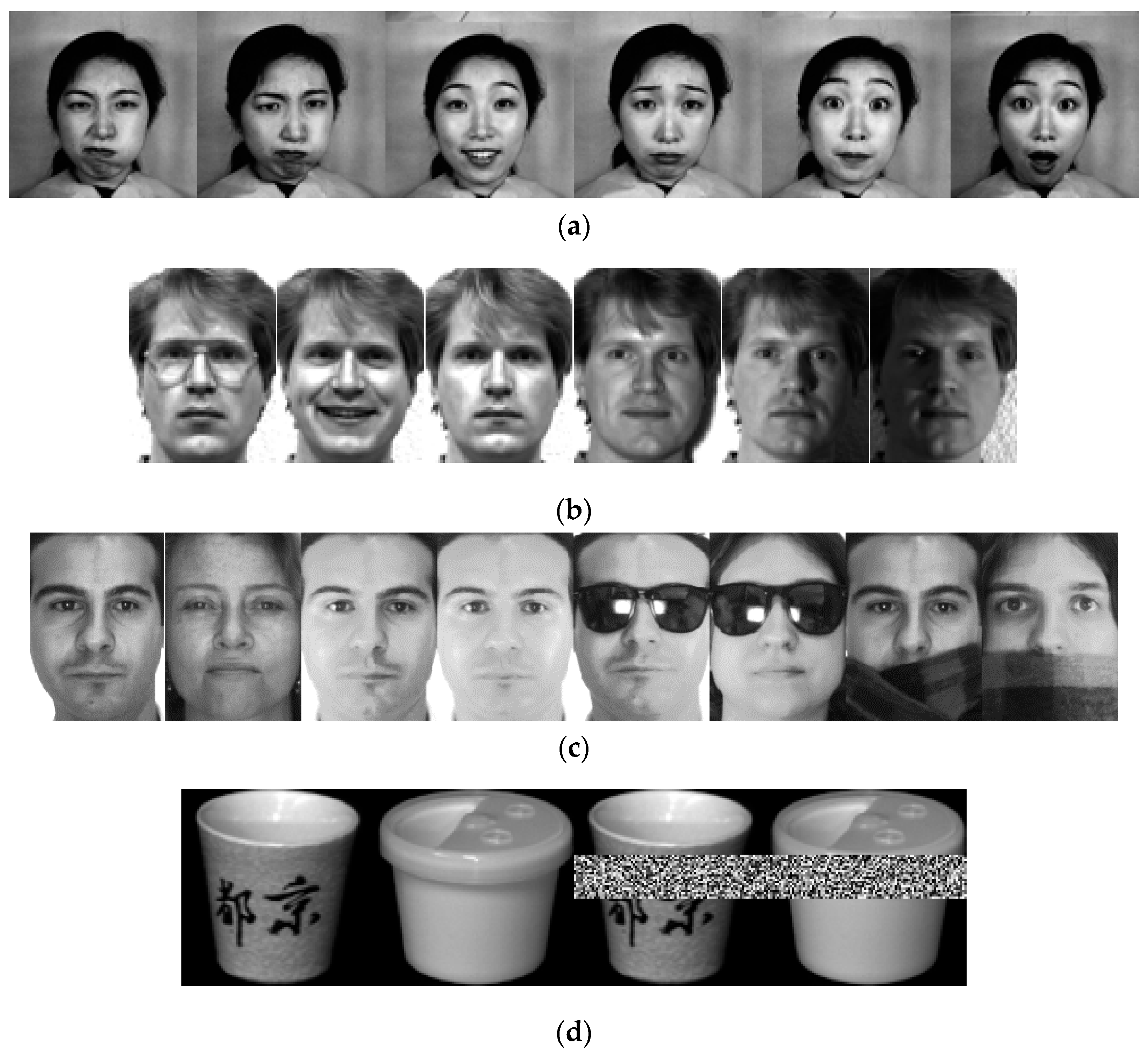
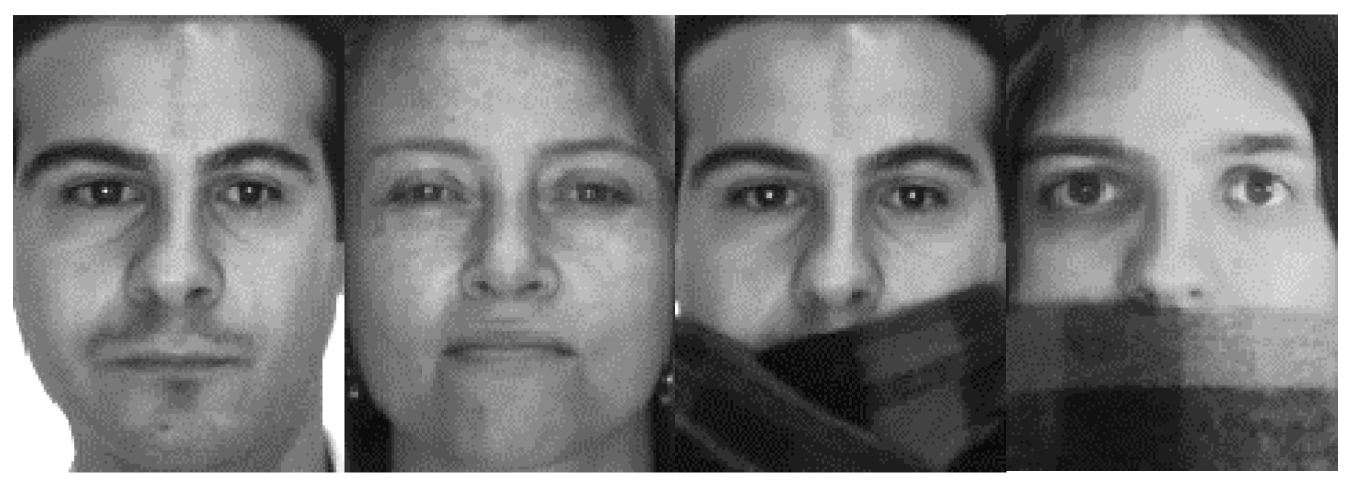
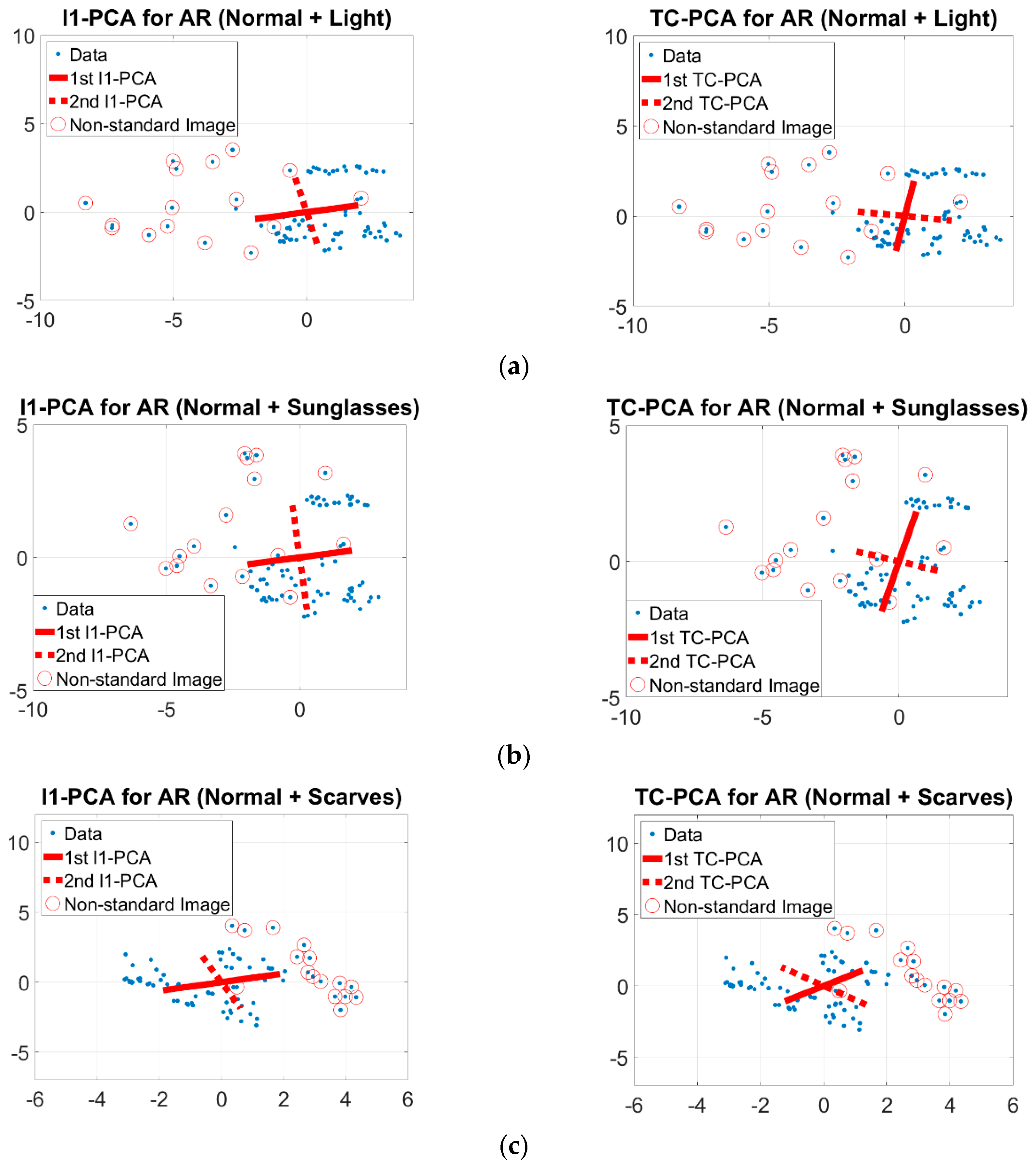
• The TC-PCA outperforms other methods in classifying non-standard images up to 8.26% for AMCR and 7.2% for AMF1-score. These results experimentally justify that the proposed method can successfully discard information given by the non-standard images such as face images under various lighting conditions. On the other hand, the performance of all methods in classifying standard images are similar (around 97%–100%), which is consistent with the findings of JAFFE face database shown in Table 1.
• The overall classification accuracy and F1-score vary with the number of testing images for the Yale face database whereas the classification performance is not sensitive to the number of testing images for the JAFFE face database. Such a difference is mainly due to the ability of each methodology in recognizing non-standard images. Our experimental results reveal that the proposed method has a superior classification performance in classifying standard images and moreover, the use of trimming set in the TC-PCA model makes the proposed method not sensitive to outliers, which can improve the non-standard image classification performance. These results indicate that the overall classification performance of all methods is comparable for the face databases with only standard images while the proposed method outperforms all other methods for the face databases consisting of both standard and non-standard images.
• The proposed method needs 9 to 21 fewer number of projection vectors to achieve high classification rates and F1-scores compared with other PCA methods. Experiments also show that the TC-PCA method usually performs better than the classifier with all dimensions (i.e., the size of an image, which is $81\times 61=4941$) and it only needs 18 to 35 dimensions to achieve good results. This may not be the case for other dimensionality reduction techniques. This shows that the TC-PCA method can effectively discard the noisy information caused by the curse of dimensionality and also better represent the key characteristics of the data.

Next, we compare the classification performance of all methods using AR face database. In this database, we perform three experiments. The first experiment (Normal + Lighting) uses all normal face images and images under lighting conditions. Similarly, the second and third experiments use all normal face images and images with sunglasses (Normal + Sunglasses) and scarves (Normal + Scarves), respectively. Note that the percentages of non-standard images in the training set when r = 1, 2, 3 and 4 are 17.65%, 20.00%, 23.08% and 27.27%, respectively and the classification results are shown in

Table 3. Comparative Classification Performance for AR Face Database (Normal + Lighting).

r		All Dim.	AMCR (Avg. Dim.) [AMF1-Score]
			PCA	HQ-PCA	l1-PCA	RPCA	OM-RPCA	AM-PCA	TC-PCA
1	Overall	0.588 ( – )	0.556 (32.30)	0.580 (52.80)	0.564 (36.10)	0.552 (32.80)	0.556 (27.40)	0.564 (32.50)	0.680 (20.80)
		[0.605]	[0.573]	[0.598]	[0.581]	[0.57]	[0.578]	[0.581]	[0.692]
	Non-standard	0.333	0.267	0.320	0.287	0.253	0.273	0.287	0.467
		[0.325]	[0.248]	[0.318]	[0.275]	[0.24]	[0.268]	[0.274]	[0.446]
	Standard	0.970	0.990	0.970	0.980	1.000	0.980	0.980	1.000
		[0.96]	[0.987]	[0.96]	[0.973]	[1.000]	[0.973]	[0.973]	[1.000]
2	Overall	0.674 ( – )	0.666 (31.60)	0.657 (26.10)	0.663 (33.90)	0.669 (31.10)	0.671 (29.10)	0.666 (36.70)	0.726 (27.70)
		[0.693]	[0.687]	[0.684]	[0.682]	[0.692]	[0.693]	[0.685]	[0.744]
	Non-standard	0.273	0.260	0.207	0.253	0.227	0.260	0.260	0.380
		[0.282]	[0.277]	[0.222]	[0.252]	[0.223]	[0.276]	[0.269]	[0.367]
	Standard	0.975	0.970	0.995	0.970	1.000	0.980	0.970	0.985
		[0.973]	[0.965]	[0.995]	[0.968]	[1.000]	[0.979]	[0.968]	[0.984]
3	Overall	0.758 ( – )	0.742 (33.40)	0.749 (32.80)	0.742 (33.10)	0.751 (39.20)	0.751 (35.30)	0.744 (35.40)	0.773 (20.90)
		[0.766]	[0.75]	[0.76]	[0.751]	[0.761]	[0.76]	[0.753]	[0.776]
	Non-standard	0.347	0.313	0.293	0.307	0.280	0.333	0.313	0.373
		[0.319]	[0.291]	[0.279]	[0.278]	[0.259]	[0.312]	[0.292]	[0.361]
	Standard	0.963	0.957	0.977	0.960	0.987	0.960	0.960	0.973
		[0.962]	[0.955]	[0.976]	[0.958]	[0.985]	[0.958]	[0.958]	[0.969]
4	Overall	0.782 ( – )	0.775 (26.30)	0.776 (28.40)	0.776 (28.50)	0.793 (23.90)	0.784 (25.20)	0.771 (23.00)	0.784 (23.90)
		[0.786]	[0.779]	[0.785]	[0.781]	[0.799]	[0.789]	[0.776]	[0.79]
	Non-standard	0.313	0.293	0.273	0.300	0.267	0.300	0.280	0.293
		[0.329]	[0.299]	[0.287]	[0.305]	[0.265]	[0.308]	[0.28]	[0.286]
	Standard	0.958	0.955	0.965	0.955	0.990	0.965	0.955	0.968
		[0.956]	[0.953]	[0.964]	[0.954]	[0.99]	[0.964]	[0.953]	[0.967]

,

Table 4. Comparative Classification Performance for AR Face Database (Normal + Sunglasses).

r		All Dim.	AMCR (Avg. Dim.) [AMF1-Score]
			PCA	HQ-PCA	l1-PCA	RPCA	OM-RPCA	AM-PCA	TC-PCA
1	Overall	0.588 ( – )	0.592 (31.70)	0.576 (40.10)	0.592 (28.30)	0.572 (36.30)	0.592 (24.40)	0.588 (29.30)	0.816 (15.10)
		[0.595]	[0.598]	[0.582]	[0.599]	[0.588]	[0.599]	[0.597]	[0.817]
	Non-standard	0.333	0.333	0.313	0.333	0.300	0.333	0.333	0.693
		[0.312]	[0.309]	[0.28]	[0.312]	[0.284]	[0.31]	[0.316]	[0.665]
	Standard	0.97	0.980	0.970	0.980	0.980	0.980	0.970	1.000
		[0.96]	[0.973]	[0.96]	[0.973]	[0.973]	[0.973]	[0.96]	[1.000]
2	Overall	0.694 ( – )	0.669 (20.90)	0.691 (31.30)	0.680 (25.60)	0.663 (38.50)	0.680 (24.80)	0.671 (27.90)	0.840 (18.10)
		[0.708]	[0.69]	[0.711]	[0.697]	[0.685]	[0.696]	[0.691]	[0.845]
	Non-standard	0.32	0.253	0.287	0.280	0.220	0.287	0.260	0.647
		[0.329]	[0.266]	[0.308]	[0.277]	[0.235]	[0.292]	[0.271]	[0.597]
	Standard	0.975	0.980	0.995	0.980	0.995	0.975	0.980	0.985
		[0.973]	[0.979]	[0.995]	[0.979]	[0.995]	[0.973]	[0.979]	[0.984]
3	Overall	0.744 ( – )	0.738 (28.60)	0.742 (45.80)	0.736 (35.60)	0.753 (35.80)	0.744 (37.20)	0.736 (34.60)	0.869 (16.10)
		[0.749]	[0.744]	[0.748]	[0.74]	[0.761]	[0.751]	[0.741]	[0.871]
	Non-standard	0.307	0.287	0.293	0.273	0.273	0.300	0.300	0.660
		[0.286]	[0.267]	[0.284]	[0.248]	[0.274]	[0.278]	[0.285]	[0.614]
	Standard	0.963	0.963	0.967	0.967	0.993	0.967	0.953	0.973
		[0.962]	[0.962]	[0.965]	[0.965]	[0.993]	[0.965]	[0.948]	[0.973]
4	Overall	0.794 ( – )	0.776 (30.60)	0.780 (29.90)	0.771 (32.70)	0.795 (31.80)	0.789 (26.10)	0.776 (33.50)	0.815 (26.70)
		[0.788]	[0.785]	[0.787]	[0.779]	[0.799]	[0.785]	[0.777]	[0.822]
	Non-standard	0.32	0.280	0.300	0.280	0.273	0.307	0.287	0.38 0
		[0.314]	[0.312]	[0.297]	[0.292]	[0.259]	[0.293]	[0.282]	[0.38]
	Standard	0.958	0.963	0.960	0.955	0.990	0.970	0.960	0.978
		[0.956]	[0.959]	[0.962]	[0.957]	[0.99]	[0.964]	[0.956]	[0.977]

and

Table 5. Comparative Classification Performance for AR Face Database (Normal + Scarves).

r		All Dim.	AMCR (Avg. Dim.) [AMF1-Score]
			PCA	HQ-PCA	l1-PCA	RPCA	OM-RPCA	AM-PCA	TC-PCA
1	Overall	0.472 ( – )	0.444 (30.90)	0.444 (37.60)	0.452 (34.80)	0.440 (39.30)	0.448 (30.30)	0.444 (26.90)	0.512 (36.30)
		[0.494]	[0.467]	[0.469]	[0.473]	[0.462]	[0.475]	[0.468]	[0.531]
	Non-standard	0.14	0.093	0.093	0.107	0.087	0.100	0.093	0.200
		[0.136]	[0.086]	[0.077]	[0.099]	[0.077]	[0.09]	[0.087]	[0.191]
	Standard	0.97	0.970	0.970	0.970	0.970	0.970	0.970	0.980
		[0.96]	[0.96]	[0.96]	[0.96]	[0.96]	[0.96]	[0.96]	[0.973]
2	Overall	0.617 ( – )	0.594 (20.90)	0.609 (30.60)	0.589 (16.30)	0.606 (36.50)	0.594 (14.90)	0.600 (24.70)	0.629 (20.70)
		[0.633]	[0.61]	[0.632]	[0.603]	[0.623]	[0.61]	[0.615]	[0.641]
	Non-standard	0.14	0.080	0.100	0.073	0.087	0.073	0.100	0.153
		[0.107]	[0.054]	[0.086]	[0.052]	[0.068]	[0.046]	[0.07]	[0.124]
	Standard	0.975	0.980	0.990	0.975	0.995	0.985	0.975	0.985
		[0.973]	[0.979]	[0.989]	[0.973]	[0.995]	[0.984]	[0.973]	[0.984]
3	Overall	0.691 ( – )	0.684 (23.10)	0.691 (30.70)	0.680 (24.40)	0.696 (31.80)	0.689 (23.10)	0.673 (24.30)	0.713 (19.40)
		[0.704]	[0.699]	[0.706]	[0.693]	[0.713]	[0.701]	[0.688]	[0.727]
	Non-standard	0.147	0.120	0.127	0.120	0.113	0.127	0.093	0.180
		[0.158]	[0.12]	[0.137]	[0.119]	[0.122]	[0.126]	[0.098]	[0.165]
	Standard	0.963	0.967	0.973	0.960	0.987	0.970	0.963	0.980
		[0.962]	[0.965]	[0.972]	[0.957]	[0.985]	[0.968]	[0.961]	[0.979]
4	Overall	0.723 ( – )	0.751 (22.60)	0.756 (32.30)	0.760 (23.40)	0.773 (21.40)	0.758 (22.30)	0.747 (25.90)	0.762 (18.70)
		[0.759]	[0.758]	[0.765]	[0.768]	[0.782]	[0.769]	[0.755]	[0.769]
	Non-standard	0.207	0.200	0.193	0.200	0.187	0.200	0.187	0.200
		[0.191]	[0.187]	[0.181]	[0.2]	[0.178]	[0.194]	[0.177]	[0.199]
	Standard	0.958	0.958	0.968	0.970	0.993	0.968	0.958	0.973
		[0.956]	[0.957]	[0.967]	[0.969]	[0.992]	[0.967]	[0.957]	[0.972]

.

Similar to the experimental results of JAFFE and Yale face databases, the proposed method performs well and its overall AMCR and AMF1-score are usually the highest. It usually outperforms other methods in classifying non-standard images for all three experiments. We remark that the proposed method performs significantly better than the other methods in recognizing non-standard images by 36%–42.7% in the “Normal + Sunglasses” experiment with r = 2. Besides, the overall AMCRs and AMF1-scores indicate that the TC-PCA again performs better than the classifier with all dimensions for any number of testing images. This may not be achieved by other PCA methods. However, the AMCRs of non-standard image classification of all methods are less than 20% in the “Normal + Scarves” experiment. The unsatisfactory non-standard image classification performance in the “Normal + Scarves” experiment suggests that more advanced facial features are necessary to correctly classifying some non-standard images.

Now, we show that the projection vectors estimated by the proposed TC-PCA can provide inter-cluster information that is beneficial to classification and clustering problems. Figure 6 shows projected data with projection vectors estimated by the $l_1$-PCA and the proposed TC-PCA in three different cases (AR (Normal + Light), AR (Normal + Sunglasses) & AR (Normal + Scarves)). Here, we select AR (Normal + Light) as an example. It is obvious that the projected data consists of two compact clusters with some outliers. The proposed TC-PCA can ignore the negative impact of the non-standard images and successfully identify the two clusters, in which the data objects in the same cluster belong to the same classes. No data objects from the same classes are assigned to the two different clusters. Moreover, the vector difference between the two cluster centers, which is the projection vector estimated by the TC-PCA, provides the inter-class information. This is important for classification and clustering problems. However, the $l_1$-PCA is greatly affected by the non-standard images and the first projection vectors are driven towards to the images. This explains why the performance of TC-PCA is better than other methods by 6% and 10%–21% better for r = 1 in AR (Normal + Scarves), AR (Normal + Light) and AR (Normal + Sunglasses).

We also compare the performance of different PCA methods for an object classification problem using Coil image database. In this experiment, the percentages of non-standard images in the training set when $r=1,2,3$ are 16.67%, 20% and 25% respectively. The classification rates are shown in

Table 6. Comparative Classification Performance for Coil.

r		All Dim.	AMCR (Avg. Dim.) [AMF1-Score]
			PCA	HQ-PCA	l1-PCA	RPCA	OM-RPCA	AM-PCA	TC-PCA
1	Overall	1.000 ( – )	0.97 (2.7)	0.985 (4.1)	0.995 (5.5)	0.98 (5.5)	0.95 (5.6)	0.995 (4.2)	1.000 (3.6)
		[1.000]	[0.973]	[0.985]	[0.995]	[0.984]	[0.956]	[0.996]	[1.000]
	Non-standard	1.000	0.94	0.97	0.99	0.96	0.9	0.99	1.000
		[1.000]	[0.962]	[1.000]	[1.000]	[0.964]	[0.93]	[0.99]	[1.000]
	Standard	1.000	1.000	1.000	1.000	1.000	1.000	1.000	1.000
		[1.000]	[1.000]	[1.000]	[1.000]	[1.000]	[1.000]	[1.000]	[1.000]
2	Overall	1.000 ( – )	0.98 (3.8)	0.983 (2.5)	0.987 (4.4)	0.967 (4.5)	0.99 (3.9)	0.987 (4.4)	1.000 (2.9)
		[1.000]	[0.98]	[0.983]	[0.988]	[0.969]	[0.99]	[0.988]	[1.000]
	Non-standard	1.000	0.94	0.95	0.96	0.9	0.97	0.96	1.000
		[1.000]	[0.951]	[0.942]	[0.963]	[0.891]	[0.971]	[0.959]	[1.000]
	Standard	1.000	1.000	1.000	1.000	1.000	1.000	1.000	1.000
		[1.000]	[1.000]	[1.000]	[1.000]	[1.000]	[1.000]	[1.000]	[1.000]
3	Overall	1.000 ( – )	0.993 (7.5)	0.995 (7.2)	0.995 (9)	0.985 (6.5)	0.995 (8.4)	0.993 (8.8)	0.998 (14.7)
		[1.000]	0.993	0.996	0.996	0.986	0.996	0.993	0.997
	Non-standard	1.000	0.97	0.98	0.98	0.94	0.98	0.97	0.99
		[1.000]	0.972	0.983	0.981	0.943	0.981	0.973	0.99
	Standard	1.000	1.000	1.000	1.000	1.000	1.000	1.000	1.000
		[1.000]	[1.000]	[1.000]	[1.000]	[1.000]	[1.000]	[1.000]	[1.000]

. The proposed method usually performs well and the overall AMCR and AMF1-score are usually the highest. Similar to the face databases, the proposed method performs better than other PCA methods in recognizing the non-standard images. Moreover, the proposed method usually uses a fewer number of projection vectors to give good results. It is also remarked that the performance of the proposed method is as good as all dimensional case. However, the proposed method uses a much lower dimension to get the same results. This shows that the proposed method can extract useful information that can effectively represent the data.

4.2. Image Clustering

In addition to face image classification, experimental results [60,61] showed that PCA can be used as a pre-processing step to enhance the accuracy of k-means clustering. In this experiment, we shall show that the clustering performance of the TC-PCA’s subspace is better than that of the other PCA’s subspaces. The experimental setting is as follows: the database is projected onto $U$ and the clustering performance is evaluated on the respective subspace. The clustering rate is obtained based on the known class labels via the following

$$\mathrm{Clustering}\mathrm{rate}=\frac{{\displaystyle \sum }best(C_i{\displaystyle \cap }{T}_{j(i)})}{\#elements},$$

(21)

where $C_i$ and $T_{j(i)}$ are ith cluster and corresponding set of training labels, respectively. In the above calculation, each cluster $C_i$ is assigned to one training label $j(i)$ only. No two or more clusters are assigned to the same training label. Since estimating the optimal number dimension for unsupervised learning problem is still a challenging research problem, we use the normalized area under the curve (NAUC) of clustering rates over the number of orthonormal projection vectors, D, to quantify the results. Note that for each value of D, we repeat the k-means clustering 30 times with the same starting vectors and the clustering result with the smallest objective value is obtained.

To evaluate the robustness of PCA methods for data clustering problem with the presence of outliers and noisy dimensions, we consider the following synthetic dataset. The dataset has 103 dimensions. The first three dimensions have 10 clusters with 100 outliers around them. Each cluster follows a normal distribution with 100 samples. Thus, the dataset has totally 1100 samples. The remaining dimensions are generated by a mixture of normal and uniform distributions. They do not carry any information about the 10 clusters. They are generated by a mixture of normal and uniform distributions. To compute the clustering rate as shown in Equation (21) of different PCA methods, we only consider the class labels of the 10 clusters and ignore the outliers in the calculation. In other words, we applied the k-means clustering algorithm to 1100 samples and only evaluate on 1000 samples, which are the 10 clusters.

Table 7. K-Means Clustering Accuracy.

	All Dim.	NAUC
		PCA	HQ-PCA	l1-PCA	RPCA	OM-RPCA	AM-PCA	TC-PCA
Synthetic Data 3	0.354	0.596	0.605	0.653	0.409	0.652	0.650	0.654
JAFFE	0.676	0.673	0.686	0.680	0.684	0.677	0.674	0.691
Yale	0.545	0.519	0.538	0.521	0.525	0.528	0.520	0.547
AR (Normal + Lighting)	0.476	0.491	0.495	0.490	0.498	0.487	0.489	0.509
AR (Normal + Sunglasses)	0.491	0.464	0.467	0.469	0.465	0.467	0.465	0.509
AR (Normal + Scarves)	0.464	0.434	0.441	0.437	0.440	0.436	0.436	0.484

³ For the synthetic data, the range of D is from 1 to 3.

shows the clustering results after applying different PCA methods. The TC-PCA method performs the best. It is 40% better than the clustering result without applying any PCA method. Besides, it performs better than other PCA methods such as RPCA nearly 35%. This implies that the proposed method is not confused by the noisy dimensions and is able to cluster the data more effectively.

Table 7 shows the comparative clustering performance for the databases used in the face image classification experiments. Generally speaking, the proposed method performs better than HQ-PCA and RPCA by around 0.5%–4.80% and the rest by around 1.78%–5.03%. The results indicate that TC-PCA’s subspace is better than the other PCA’s subspaces for clustering. Moreover, the NAUC of the proposed method is higher than the clustering results with all dimensions in all five experiments, which may not be achieved by other PCA methods.

4.3. Parameter Study

In this section, we study the effectiveness of the two parameters of SPVEA. First, we study the effectiveness of the trimming parameter, $p$, which is set as 75 in all the experiments. Then, we study the robustness of the cluster center initialization of the SPVEA.

4.3.1. Effectiveness of the Trimming Parameter

In this subsection, we shall have the parameter study of TC-PCA, including the parameter of trimming set, p and the number of testing images selected for each individual in the standard part, r, to the classification performance, as shown in

Table 8. Classification Performance (averaged maximum classification rate (AMCR)) of TC-PCA for Various Parameters.

p	Database	r
		1	2	3	4
95	JAFFE	1.000	0.995	0.993	0.988
	Yale	0.643	0.737	0.806	0.811
	AR (Normal + Lighting)	0.568	0.663	0.753	0.787
	AR (Normal + Sunglasses)	0.604	0.683	0.751	0.784
	AR (Normal + Scarves)	0.448	0.600	0.693	0.742
90	JAFFE	1.000	0.995	0.993	0.988
	Yale	0.646	0.744	0.802	0.810
	AR (Normal + Lighting)	0.556	0.657	0.749	0.787
	AR (Normal + Sunglasses)	0.596	0.683	0.760	0.787
	AR (Normal + Scarves)	0.472	0.600	0.702	0.742
85	JAFFE	1.000	0.995	0.997	0.990
	Yale	0.654	0.739	0.796	0.805
	AR (Normal + Lighting)	0.588	0.709	0.753	0.786
	AR (Normal + Sunglasses)	0.652	0.714	0.782	0.800
	AR (Normal + Scarves)	0.476	0.603	0.722	0.744
80	JAFFE	1.000	0.995	0.997	0.99
	Yale	0.681	0.729	0.794	0.816
	AR (Normal + Lighting)	0.604	0.726	0.747	0.789
	AR (Normal + Sunglasses)	0.820	0.803	0.791	0.820
	AR (Normal + Scarves)	0.504	0.620	0.716	0.747
75	JAFFE	1.000	0.990	0.990	0.995
	Yale	0.681	0.763	0.809	0.816
	AR (Normal + Lighting)	0.680	0.726	0.773	0.784
	AR (Normal + Sunglasses)	0.816	0.840	0.869	0.815
	AR (Normal + Scarves)	0.512	0.629	0.713	0.762

. Here, we choose p = 75, 80, 85, 90, 95 and r = 1, 2, 3, 4. There are two important points that can be observed from Table 8. First, the classification performance is not sensitive to r for the JAFFE face database whereas the AMCR increases with r for the Yale and AR face databases at the same value of p, which are consistent with our previous results in Section 4.1 (see also discussions in the same section). Second, the classification performance for the JAFFE face database is stable for any value of p whereas the AMCR improves from p = 95 to p = 75 for Yale and AR face databases at the same value of r. These results further justify that the AMCR for the databases with both standard and non-standard images increases gradually by removing a portion of outlier images in the training set, which in turn, reveals the effectiveness of trimming set in the TC-PCA model. It is important to note that we fix the parameter D from 1 to 70 for image classification and clustering but our experimental results show that increasing the value of D to more than 70 does not affect the AMCR and NAUC. Other than the above analysis, we also find that the parameter setting $p=75$ is the best for these face databases. We compare the performance of this setting with parameter estimation using the holdout method as described in Section 4.1, which has been used to estimate the optimal number of projection vectors. The result is shown in

Table 9. Classification Performance (AMCR) of TC-PCA with Holdout Estimation for the Trimming Parameter.

Database	r
	1	2	3	4
JAFFE	1.000	0.975	0.987	0.995
Yale	0.659	0.744	0.809	0.812
AR (Normal + Lighting)	0.632	0.683	0.773	0.795
AR (Normal + Sunglasses)	0.812	0.860	0.829	0.802
AR (Normal + Scarves)	0.480	0.617	0.709	0.767

. We can see that other than $r=2$ for AR (Normal + Sunglasses) and $r=4$ for AR (Normal + Scarves), the parameter setting $p=75$ performs better than automatic parameterization. This shows that the parameter setting $p=75$ is the best for these face databases.

4.3.2. Sensitivity Analysis of Cluster Centers Initialization of the SPVEA

In this subsection, we study the robustness of cluster center initialization procedure of the SPVEA. We apply SPVEA 30 times with different sets of initial guesses to each of the four face databases with $r=1$ and obtain projection matrices. We measure the difference among these projection matrices by the following formula

$$Diff(D_V)=std({\Vert V{(i)}^{T}V(j)\Vert }_1/D_V),$$

(22)

where $V(i)$ is the projection matrices obtained by SPVEA with ith set of initial guesses and $D_v$ is the number of projection vectors of the projection matrix. $Diff(D_V)$ is to compute the standard deviation of all the dot products of any two projection matrices obtained by different sets of initial guesses. If all projection matrices $V(i)$ are similar to each other, the ${\Vert V{(i)}^{T}V(j)\Vert }_1$ will be close to one and thus, obtain a very small standard deviation.

Table 10. Difference Scores Among Different Initialization of Single Projection Vector Extraction Algorithm (SPVEA).

Database	No. of Projection Vectors
	1	10	20
JAFFE	$1.606\times {10}^{-4}$	$3.109\times {10}^{-3}$	$5.829\times {10}^{-4}$
Yale	$1.337\times {10}^{-3}$	$3.330\times {10}^{-3}$	$5.149\times {10}^{-4}$
AR (Normal + Lighting)	$1.068\times {10}^{-16}$	$2.203\times {10}^{-3}$	$5.394\times {10}^{-4}$
AR (Normal + Sunglasses)	$1.068\times {10}^{-16}$	$2.373\times {10}^{-3}$	$5.469\times {10}^{-4}$
AR (Normal + Scarves)	$1.068\times {10}^{-16}$	$2.374\times {10}^{-3}$	$5.173\times {10}^{-4}$

below shows the values of $Diff(D_V)$ to the four face databases under three settings: $D_V=1, D_V=10$ and $D_V=20$. We can see that all values are very small and close to zero. This shows that the projection vectors generated by SPVEA is robust to cluster center initialization.

4.4. Discussions for Large Number of Outliers

In this subsection, we investigate the case when the number of outliers exceeds 50%. We set $r=8$ for the four face databases. That means there are around 60% non-standard images in each situation. The results are shown in

Table 11. Comparative Classification Performance of Different PCA Methods with Around 60% Outliers.

Database		All Dim.	AMCR (Avg. Dim.) [AMF1-Score]
			PCA	HQ-PCA	l1-PCA	RPCA	OM-RPCA	AM-PCA	TC-PCA
Yale	Overall	0.804 ( – )	0.80 (25)	0.758 (27.5)	0.797 (22.70)	0.821 (26.80)	0.80 (28.70)	0.802 (24.30)	0.806 (31.40)
		[0.799]	[0.796]	[0.754]	[0.792]	[0.821]	[0.796]	[0.798]	[0.801]
	Non-standard	0.339	0.33	0.317	0.335	0.313	0.335	0.33	0.352
		[0.316]	[0.308]	[0.3]	[0.318]	[0.3]	[0.315]	[0.304]	[0.325]
	Standard	0.907	0.904	0.856	0.899	0.934	0.903	0.906	0.907
		[0.898]	[0.897]	[0.845]	[0.89]	[0.93]	[0.894]	[0.899]	[0.897]
AR (Normal + Lighting)	Overall	0.785 ( – )	0.702 (13.10)	0.648 (13.45)	0.702 (14.50)	0.742 (14.40)	0.739 (17.15)	0.746 (15.10)	0.71 (12.75)
		[0.781]	[0.697]	[0.64]	[0.695]	[0.742]	[0.733]	[0.741]	[0.705]
	Non-standard	0.367	0.283	0.257	0.283	0.24	0.303	0.297	0.28
		[0.313]	[0.267]	[0.242]	[0.267]	[0.225]	[0.282]	[0.283]	[0.253]
	Standard	0.874	0.792	0.732	0.791	0.849	0.832	0.843	0.802
		[0.868]	[0.781]	[0.719]	[0.778]	[0.846]	[0.822]	[0.833]	[0.792]
AR (Normal + Sunglasses)	Overall	0.793 ( – )	0.774 (14.90)	0.634 (9.80)	0.731 (13.30)	0.726 (14.20)	0.754 (16.20)	0.712 (14.20)	0.74 (12.90)
		[0.79]	[0.771]	[0.622]	[0.723]	[0.723]	[0.752]	[0.708]	[0.737]
	Non-standard	0.427	0.427	0.313	0.38	0.32	0.413	0.367	0.353
		[0.405]	[0.391]	[0.293]	[0.335]	[0.29]	[0.384]	[0.324]	[0.335]
	Standard	0.871	0.849	0.703	0.806	0.813	0.827	0.786	0.823
		[0.865]	[0.844]	[0.687]	[0.795]	[0.804]	[0.822]	[0.779]	[0.814]
AR (Normal + Scarves)	Overall	0.767 ( – )	0.645 (9.60)	0.581 (10.10)	0.582 (7.40)	0.486 (7.90)	0.676 (11.20)	0.655 (10.9)	0.669 (11.60)
		[0.767]	[0.643]	[0.578]	[0.578]	[0.48]	[0.674]	[0.656]	[0.667]
	Non-standard	0.28	0.213	0.187	0.167	0.18	0.253	0.227	0.2
		[0.271]	[0.185]	[0.158]	[0.158]	[0.154]	[0.242]	[0.219]	[0.191]
	Standard	0.871	0.737	0.666	0.671	0.551	0.767	0.747	0.77
		[0.865]	[0.735]	[0.662	[0.662]	[0.543]	[0.76]	[0.742]	[0.764]

. We can observe that the performance of any PCA method is usually not as good as the one without applying any PCA method. The reason may be that current PCA methods attempt to find the common components that can best represent the data. Given the scatter nature of outliers, this can confuse most PCA methods. Although the proposed method does not perform as good as the one without applying any PCA method, it performs the best, 2nd best and 3rd best among the PCA methods in Yale, AR (Normal + Lighting), AR (Normal + Sunglasses) and AR (Normal + Scarves) respectively.

5. Conclusions

In this paper, we show that the l₁-PCA is equivalent to the two-group k-means clustering model. This equivalence indicates that the projection vector of the $l_1$-PCA is the vector difference between the two cluster centers obtained by the clustering algorithm. In other words, the projection vector incorporates inter-cluster information, which is beneficial to distinguish data objects from different classes. However, this equivalence also indicates that the $l_1$-PCA may be sensitive to outlier. To overcome this limitation, a novel trimmed-clustering based l₁-PCA (TC-PCA) model is proposed. The TC-PCA is developed by incorporating a trimming set into the aforementioned clustering model so that the proposed method is not sensitive to outliers. In addition, the TC-PCA does not require data centralization procedure to obtain the projection vectors. Furthermore, we mathematically prove that the proposed TC-PCA algorithm converges. Comparative experimental results with current existing PCA approaches show that our method achieves remarkable success in face image classification and clustering problems.

While our proposed method provides promising classification and clustering results, we shall study the following as future work:

• The proposed TC-PCA model works well in image classification and clustering. More analysis of the proposed method to different applications such as video surveillance and image segmentation should be done.
• We adopt the hold-out method to estimate the optimal number of projection vectors for classification problems. However, this method did not give the best solutions in the experiments. A more robust estimation should be developed.
• Many PCA methods such as the traditional PCA can be extended to the so-called 2D-PCA. Like these methods, a nature extension of the proposed method to 2D-PCA should be investigated.

References

1. Nam, G.; Heeseung, C.; Junghyun, C.; Kim, I. PSI-CNN: A pyramid-based scale-invariant CNN architecture for face recognition robust to various image resolutions. Appl. Sci. 2018, 8, 1561. [Google Scholar] [CrossRef]
2. Basaran, E.; Gökmen, M.; Kamasak, M. An efficient multiscale scheme using local zernike moments for face recognition. Appl. Sci. 2018, 8, 827. [Google Scholar] [CrossRef]
3. Shnain, N.; Hussain, Z.; Lu, S. A feature-based structural measure: An image similarity measure for face recognition. Appl. Sci. 2017, 7, 786. [Google Scholar] [CrossRef]
4. Liu, Z.; Song, R.; Zeng, D.; Zhang, J. Principal components adjusted variable screening. Comput. Stat. Data Anal. 2017, 110, 134–144. [Google Scholar] [CrossRef]
5. Julie, J.; Francois, H. Selecting the number of components in PCA using cross-validation approximations. Comput. Stat. Data Anal. 2012, 56, 1869–1879. [Google Scholar]
6. Yang, J.; Zhang, D.; Frangi, A.F.; Yang, J.-Y. Two-dimensional PCA: A New approach to appearance-based face representation and recognition. IEEE Trans. Pattern Anal. Mach. Intell. 2004, 26, 131–137. [Google Scholar] [CrossRef] [PubMed]
7. Zhang, F.; Yang, J.; Qian, J.; Xu, Y. Nuclear norm-based 2-DPCA for extracting features from images. IEEE Trans. Neural Netw. Learn. Syst. 2015, 26, 2247–2260. [Google Scholar] [CrossRef]
8. Wang, Q.; Gao, Q. Two-dimensional PCA with F-norm minimization. In Proceedings of the AAAI Conference on Artificial Intelligence, San Francisco, CA, USA, 4–9 February 2017; pp. 2718–2724. [Google Scholar]
9. Gao, Q.; Gao, F.; Zhang, H.; Hao, X.-J.; Wang, X. Two-dimensional maximum local variation based on image euclidean distance for face recognition. IEEE Trans. Image Process. 2013, 22, 3807–3817. [Google Scholar] [PubMed]
10. Lai, Z.; Xu, Y.; Yang, J.; Tang, J.; Zhang, D. Sparse tensor discriminant analysis. IEEE Trans. Image Process. 2013, 22, 3904–3915. [Google Scholar] [PubMed]
11. Gao, Q.; Wang, Q.; Huang, Y.; Gao, X.; Hong, X.; Zhang, H. Dimensionality reduction by integrating sparse representation and fisher criterion and its applications. IEEE Trans. Image Process. 2015, 24, 5684–5695. [Google Scholar] [CrossRef]
12. Navarrete, P.; Ruiz-del-Solar, J. Analysis and comparison of eigenspace-based face recognition approaches. Int. J. Pattern Recognit. Artif. Intell. 2002, 16, 817–830. [Google Scholar] [CrossRef]
13. Brooks, J.P.; Dulá, J.H.; Boone, E.L. A Pure L1-norm principal component analysis. Comput. Stat. Data Anal. 2013, 61, 83–98. [Google Scholar] [CrossRef] [PubMed]
14. Kwak, N. Principal component analysis based on L1-norm maximization. IEEE Trans. Pattern Anal. Mach. Intell. 2008, 30, 1672–1680. [Google Scholar] [CrossRef]
15. Candes, E.; Li, X.; Ma, Y.; Wright, J. Robust principal component analysis? J. ACM 2011, 58, 11. [Google Scholar] [CrossRef]
16. Xu, H.; Caramanis, C.; Sanghavi, S. Robust PCA by outlier pursuit. IEEE Trans. Inf. Theory 2012, 58, 3047–3064. [Google Scholar] [CrossRef]
17. Wright, J.; Ganesh, A.; Rao, S.; Ma, Y. Robust principal component analysis: Exact recovery of corrupted low-rank matrices via convex optimization. Adv. Neural Inf. Process. Syst. 2009, 22, 2080–2088. [Google Scholar]
18. McCoy, M.; Tropp, J. Two proposals for robust PCA using semidefinite programming. Electron. J. Stat. 2011, 5, 1123–1160. [Google Scholar] [CrossRef]
19. Nie, F.; Huang, H.; Ding, C.; Luo, D.; Wang, H. Robust principal component analysis with non-greedy l1-norm maximization. In Proceedings of the International Joint Conference on Artificial Intelligence, Barcelona, Spain, 16–22 July 2011; pp. 1433–1438. [Google Scholar]
20. Zhou, T.; Tao, D. Double shrinking sparse dimension deduction. IEEE Trans. Image Process. 2013, 22, 244–257. [Google Scholar] [CrossRef] [PubMed]
21. Markopoulos, P.P.; Karystinos, G.N.; Pados, D.A. Optimal algorithms for L1-subspace signal processing. IEEE Trans. Signal Process. 2014, 62, 5046–5058. [Google Scholar] [CrossRef]
22. Markopoulos, P.P.; Kundu, S.; Chamadia, S.; Pados, D.A. Efficient L1-norm principal-component analysis via bit flipping. IEEE Trans. Signal Process. 2017, 65, 4252–4264. [Google Scholar] [CrossRef]
23. Kwak, N. Principal component analysis by Lp-norm Maximization. IEEE Trans. Cybern. 2014, 44, 594–609. [Google Scholar] [CrossRef]
24. Luo, M.; Nie, F.; Chang, X.; Yang, Y.; Hauptmann, A.; Zheng, Q. Avoiding optimal mean robust PCA/2DPCA with non-greedy l1-norm maximization. In Proceedings of the International Joint Conference on Artificial Intelligence, New York, NY, USA, 9–16 July 2016; pp. 1802–1808. [Google Scholar]
25. Luo, M.; Nie, F.; Chang, X.; Yang, Y.; Hauptmann, A.G.; Zheng, Q. Avoiding optimal mean l2,1-norm maximization-based robust PCA for reconstruction. Neural Comput. 2017, 29, 1124–1150. [Google Scholar] [CrossRef]
26. Ke, Q.; Kanade, T. Robust L1-norm factorization in the presence of outliers and missing data by alternative convex programming. In Proceedings of the IEEE Computer Society Conference on Computer Vision and Pattern Recognition (IEEE CVPR), San Diego, CA, USA, 20–25 June 2005; pp. 739–746. [Google Scholar]
27. Meng, D. Divide-and-conquer method for l1-norm matrix factorization in the presence of outliers and missing data. arXiv 2012, arXiv:1202.5844. [Google Scholar]
28. Nie, F.; Yuan, J.; Huang, H. Optimal mean robust principal component analysis. In Proceedings of the International Conference on Machine Learning, Beijing, China, 21–26 June 2014; pp. 1062–1070. [Google Scholar]
29. He, R.; Hu, B.G.; Zheng, W.S.; Kong, X.W. Robust principal component analysis based on maximum correntropy criterion. IEEE Trans. Image Process. 2011, 20, 1485–1494. [Google Scholar]
30. Wang, Q.; Gao, Q.; Gao, X.; Nie, F. l2,p-norm based PCA for image recognition. IEEE Trans. Image Process. 2018, 27, 1336–1346. [Google Scholar] [CrossRef]
31. Li, X.; Pang, Y.; Yuan, Y. L1-norm-based 2DPCA. IEEE Trans. Syst. Man Cybern. Part B 2010, 40, 1170–1175. [Google Scholar]
32. Ju, F.; Sun, Y.; Gao, J.; Hu, Y.; Yin, B. Image outlier detection and feature extraction via l1-norm-based 2D probabilistic PCA. IEEE Trans. Image Process. 2015, 24, 4834–4846. [Google Scholar] [CrossRef]
33. Zhong, F.; Zhang, J. Linear discriminant analysis based on L1-norm maximization. IEEE Trans. Image Process. 2013, 22, 3018–3027. [Google Scholar] [CrossRef]
34. Liu, Y.; Gao, Q.; Miao, S.; Gao, X.; Nie, F.; Li, Y. A non-greedy algorithm for l1-norm LDA. IEEE Trans. Image Process. 2017, 26, 684–695. [Google Scholar] [CrossRef]
35. Wang, R.; Nie, F.; Yang, X.; Gao, F.; Yao, M. Robust 2DPCA with non-greedy L1-norm maximization for image analysis. IEEE Trans. Cybern. 2015, 45, 1108–1112. [Google Scholar] [CrossRef]
36. Ding, X.; He, L.; Carin, L. Bayesian robust principal component analysis. IEEE Trans. Image Process. 2011, 20, 3419–3430. [Google Scholar] [CrossRef]
37. Parker, J.T.; Schniter, P.; Cevher, V. Bilinear generalized approximate message passing—Part I: Derivation. IEEE Trans. Signal Process. 2014, 62, 5839–5853. [Google Scholar] [CrossRef]
38. Parker, J.T.; Schniter, P.; Cevher, V. Bilinear generalized approximate message passing—Part II: Application. IEEE Trans. Signal Process. 2014, 62, 5854–5867. [Google Scholar] [CrossRef]
39. Khan, Z.; Shafait, F.; Mian, A. Joint group sparse PCA for compressed hyperspectral imaging. IEEE Trans. Image Process. 2015, 24, 4934–4942. [Google Scholar] [CrossRef]
40. Zhang, Z.; Li, F.; Zhao, M.; Zhang, L.; Yan, S. Joint low-rank and sparse principal feature coding for enhanced robust representation and visual classification. IEEE Trans. Image Process. 2016, 25, 2429–2443. [Google Scholar] [CrossRef]
41. Wang, N.; Yao, T.; Wang, J.; Yeung, D. A probabilistic approach to robust matrix factorization. In European Conference on Computer Vision; Springer: Berlin/Heidelberg, Germany, 2012; pp. 126–139. [Google Scholar]
42. Wang, N.; Yeung, D. Bayesian robust matrix factorization for image and video processing. In Proceedings of the IEEE International Conference on Computer Vision, Sydney, Australia, 1–8 December 2013. [Google Scholar]
43. Zhao, Q.; Meng, D.; Xu, Z.; Zuo, W.; Zhang, L. Robust principal component analysis with complex noise. In Proceedings of the 31st International Conference on Machine Learning, Beijing, China, 21–26 June 2014. [Google Scholar]
44. Xue, J.; Zhao, Y.; Liao, W.; Chan, J. Total variation and rank-1 constraint RPCA for background subtraction. IEEE Access 2018, 6, 49955–49966. [Google Scholar] [CrossRef]
45. Huber, P.J.; Ronchetti, E.M. Robust Statistics, 2nd ed.; Wiley: Hoboken, NJ, USA, 2009. [Google Scholar]
46. Mittal, S.; Anand, S.; Meer, P. Generalized projection-based M-estimator. IEEE Trans. Pattern Anal. Mach. Int. 2012, 34, 2351–2364. [Google Scholar] [CrossRef]
47. Mittal, S.; Anand, S.; Meer, P. Generalized projection-based M-estimator: Theory and application. In Proceedings of the IEEE Conference on Computer Vision and Pattern Recognition (CVPR), Colorado Springs, CO, USA, 20–25 June 2011; pp. 2689–2696. [Google Scholar]
48. Fauconnier, C.; Haesbroeck, G. Outliers detection with the minimum covariance determinant estimator in practice. Stat. Methodol. 2009, 6, 363–379. [Google Scholar] [CrossRef]
49. Rousseeuw, P.J.; Driessen, K.V. A fast algorithm for the minimum covariance determinant estimator. Technometrics 1999, 41, 212–223. [Google Scholar] [CrossRef]
50. Zhang, J.; Li, G. Breakdown point properties of location M-estimators. Ann. Stat. 1998, 26, 1170–1189. [Google Scholar]
51. Pearson, K. On lines and planes of closest fit to systems of points in space. Lond. Edinb. Dublin Philos. Mag. J. Sci. 1901, 2, 559–572. [Google Scholar] [CrossRef]
52. Bengio, Y.; Courville, A.; Vincent, P. Representation learning: A review and new perspectives. IEEE Trans. Pattern Anal. Mach. Intell. 2013, 35, 1798–1828. [Google Scholar] [CrossRef] [PubMed]
53. The Japanese Female Facial Expression (JAFFE) Database. Available online: http://www.kasrl.org/jaffe.html (accessed on 27 July 2018).
54. The Yale Face Database. Available online: http://cvc.cs.yale.edu/cvc/projects/yalefaces/yalefaces.html (accessed on 27 July 2018).
55. Martinez, A.M.; Benavente, R. The AR Face Database; CVC Technical Report 24; Computer Vision Centar: Barcelona, Spain, 1998. [Google Scholar]
56. Columbia University Image Library. Available online: http://www.cs.columbia.edu/CAVE/software/softlib/coil-20.php (accessed on 27 July 2018).
57. Nene, S.A.; Nayar, S.K.; Murase, H. Columbia Object Image Library (COIL-20); Technical Report CUCS-005-96; Department of Computer Science, Columbia University: New York, NY, USA, 1996. [Google Scholar]
58. Wang, X.; Tang, X. A unified framework for subspace face recognition. IEEE Trans. Pattern Anal. Mach. Intell. 2004, 26, 1222–1228. [Google Scholar] [CrossRef] [PubMed]
59. Chen, G.; Florero-Salinas, W.; Li, D. Simple, fast and accurate hyper-parameter tuning in Gaussian-kernel SVM. In Proceedings of the International Joint Conference on Neural Networks, Budapest, Hungary, 14–19 July 2017; pp. 348–355. [Google Scholar]
60. Ding, C.; Zhou, D.; He, X.; Zha, H. R1-PCA: Rotational Invariant L1-norm principal component analysis for robust subspace factorization. In Proceedings of the International Conference on Machine Learning, Pittsburgh, PA, USA, 25–19 June 2006; pp. 281–288. [Google Scholar]
61. Ding, C.; He, X. K-means clustering via principal component analysis. In Proceedings of the International Conference on Machine Learning, Banff, Canada, 4–8 July 2004; pp. 225–232. [Google Scholar]
Figure 1. Example frontal faces and faces with scarves.
Applsci 09 01562 g001
Figure 2. Illustration of the clustering property of the principal component analysis ( l 1 -PCA).
Applsci 09 01562 g002
Figure 3. (a) First projection vector obtained by l1-PCA. (b) Cluster centers obtained by two-group k -means clustering model.
Applsci 09 01562 g003
Figure 4. First projection vectors obtained by (a) l1-PCA and (b) trimmed clustering principal component analysis (TC-PCA) for the dataset with outliers.
Applsci 09 01562 g004
Figure 5. (a) JAFFE face database: images with various facial expressions. (b) Yale face database: 1st–3rd images: normal faces; 4th–6th images: faces under various lighting conditions. (c) AR face database: 1st–2nd images: normal faces; 3th–4th images: faces under various lighting conditions; 5th–6th images: faces with sunglasses; 7th–8th images: faces with scarves. (d) COIL-20 image database: 1st–2nd images: normal objects; 3rd–4th images: objects with artificial blocking.
Applsci 09 01562 g005
Figure 6. The 1st and 2nd projection vectors obtained by l 1 -PCA and TC-PCA for AR Face Database with (a) Normal + Lighting, (b) Normal + Sunglasses and (c) Normal + Scarves.
Applsci 09 01562 g006