Life-Cycle Optimization of a Chiller Plant with Quantified Analysis of Uncertainty and Reliability in Commercial Buildings

Featured Application

Proper design of a chiller plant is considered as one of the most effective ways to reduce the energy consumption of commercial buildings. Due to the improper treatment of uncertainty and reliability, existing design methods in practice often result in oversized systems. This paper proposes a design optimization method for chiller plants based on life-cycle total cost minimization with quantified analysis of uncertainty and reliability. It can ensure a chiller plant operates at its high efficient region under various cooling load conditions and provide sufficient cooling capacity even some equipment/systems with failures.

Abstract

Conventional and most optimal design methods for chiller plants often address the annual cooling load distribution of buildings and their peak cooling loads based on typical meteorological year (TMY) data, while the peak cooling load only appears a few times during the life-cycle and the sized chiller plant usually operates within its low efficient region. In this paper, a robust optimal design method based on life-cycle total cost was employed to optimize the design of a chiller plant with quantified analysis of uncertainty and reliability. By using the proposed design method, the optimized chiller plant can operate at its highly efficient region under various cooling load conditions, and provide sufficient cooling capacity even alongside some equipment/systems with failures. The minimum life-cycle total cost, which consists of the capital cost, operation, and availability-risk cost, can be achieved through optimizing the total cooling capacity and the numbers/sizes of chillers. A case study was conducted to illustrate the detailed implementation process of the proposed method. The performance of this design method was evaluated by comparing with that of other design methods.

1. Introduction

In Hong Kong, heating, ventilation, and air conditioning (HVAC) systems account for about 40% of the total energy consumed in the building sector [1]. Among all HVAC components, a chiller plant occupies up to 50% of the total energy consumption, which plays a critical role in determining the energy performance of the whole HVAC system [2]. Proper design of a chiller plant is considered as one of the most effective ways to reduce the energy consumption of the chiller plant, which has attracted increasing attention worldwide.

1.1. Conventional and Optimal Design of a Chiller Plant

The size and configuration of a chiller plant are two of the most important influencing factors of energy performance, which determine whether the HVAC system could operate within its high efficient region or not [3]. The American Society of Heating, Refrigerating and Air-Conditioning Engineers (ASHRAE) handbook [4] introduced a conventional chiller plant design method, which mainly focused on how to fulfill the peak cooling load at a rated operating point. In order to determine the size of a chiller plant, two typical methods for estimating the building cooling load are suggested as follows [5]:

• The cooling load of a typical design day is determined according to the statistic historical outdoor weather conditions and maximum boundaries.
• Simulation software such as EnergyPlus [6] and TRNSYS [7] are employed to generate the annual cooling load distribution according to typical meteorological year (TMY) data, behaviors of occupants, schedules of plug-in appliances, lightings, etc.

Based on the above-mentioned methods, the determination process of chiller plant cooling capacity could be considered as a deterministic model based on simulation [8]. In fact, there are many inevitable differences between the actual operating parameters (e.g., weather conditions, internal heat gains, and indoor occupants) and those used in the design calculation (usually referring as uncertainties), which will result in a large deviation between the actual cooling load and the design cooling load [9]. Generally, designers usually prefer to size the chiller plant with a larger cooling capacity than the maximum cooling load (i.e., adding a safety factor) to make sure that the chiller plant could supply sufficient cooling capacity in satisfying the cooling demand under a series of cooling load scenarios for safety consideration [10,11]. This might easily result in oversizing problems, which reflect as that chiller plant frequently operates within its low efficient region, and thus a large amount of energy is wasted [12,13,14].

Since full load conditions (i.e., peak load) occupy a very small proportion of the whole cooling season, some studies have proposed that more attention should be paid to part load conditions, which also requires the chiller plant to serve at its high efficient region [9]. A chiller plant consisting of multiple chillers is considered as an effective option to improve efficiency by combining the optimal sequence control during operation [15,16,17,18]. When the actual cooling load is less than the peak cooling load, some chillers could be switched off and then the operating chillers can operate at a relatively high part load ratio (PLR) within their high efficient regions. The use of high efficiency chillers is considered as another effective way to ensure the operational performance of a chiller plant at high levels [19]. For instance, variable-speed chillers that have good performance characteristics even under very low part load conditions are recommended to be employed when the chiller plant operates at part load conditions frequently [20]. In addition, the optimization of chiller plants can also be achieved by integrating hybrid chillers with different types of compressors and/or driven by different energy sources, so that all operating chillers can operate within their optimal loading ranges [21].

1.2. Uncertainty Research for Building Energy System

As mentioned above, the conventional and optimal design methods often focus on annual cooling load distribution and peak values based on “pre-determined” input parameters [11,22]. However, by considering the various uncertain input parameters, the actual cooling load conditions are seldom the same as the specified conditions (i.e., using the specified input parameters). Thus, the sized chiller plant is very likely to operate at its low efficient region due to low part load ratios [22,23]. For the sake of addressing the impacts caused by the uncertain input parameters, some researchers tried to find out a resilient and sustainable design method by considering uncertainties [24,25]. Pettersen [26] investigated building envelops and inhabitants, as well as the power consumption of buildings by considering the uncertainties of the weather conditions. The case study indicated that the power consumption changed within a range of ±25%–40% when considering uncertainties. Li et al. [27] and Smith et al. [28] presented a sensitivity analysis on a combined cooling, heating and power (CCHP) system by considering the quantified uncertainties in models, as well as in inputs. The impact of such uncertainties on estimating the energy performance of the CCHP system was analyzed in case studies. Menassa [29] proposed a quantitative method in considering different levels of uncertainties to evaluate the investment feasibility on the retrofits of existing buildings.

1.3. Reliability Research for Building Energy System

The reliability analysis is very important in building an energy system design, which determines whether the system has sufficient capability to fulfill the requirements for both normal conditions (e.g., the design capacity is more than the operating duty) and abnormal conditions (e.g., the components’ failure) [30,31]. By considering the benefits of economic (i.e., the reduction of energy consumption and maintenance cost) and environmental management, the significance of reliability parameters was evaluated and emphasized by Peruzzi et al. [32]. The operation and maintenance characteristics of a HVAC system, which have an impact on the satisfaction of occupants, were studied by Au-Yong et al. [33]. A relationship between the satisfaction of occupants and the characteristics of a HVAC system was established based on questionnaire investigations. A regressed prediction model was also developed accordingly. Kwak et al. [34] developed a quantitative method according to the reliability analysis of air-conditioning systems, in order to estimate the optimum inspection period for condition-based maintenance in commercial buildings. Among these studies mentioned above, a very small number of studies have considered components’ reliabilities by adopting quantitative methods in a HVAC system design process. In order to optimize the cooling water system configuration, Cheng et al. [35] developed a robust optimal design method by considering the system uncertainties and reliabilities. The results showed that the sized pumping system could have enough capability to supply the cooling and operate within its efficient region.

In summary, most conventional and optimal chiller design methods are based on the annual cooling load under predefined conditions, which may ensure the designed systems operate at a satisfactory performance when the actual operating conditions are the same or close to the predefined conditions. However, in most occasions the actual conditions often deviate from the predefined conditions due to the inevitable uncertainties and equipment failures in the real world. In order to address the impact of uncertainties of design inputs and reliability of the components in operation, this study presents an optimal and robust design method for a chiller plant by considering both uncertainty and reliability simultaneously in quantitative ways. Different from previous studies that mainly addressed the cooling load distribution and its peak value in a typical year [36,37,38], in this paper, the distribution of the cooling load is calculated based on a large number of cooling load scenarios while considering a series of uncertainties. Monte Carlo simulation is employed to simulate these scenarios of cooling load for generating a more representative cooling load distribution. In contrast to the previous studies that mainly address the energy efficiency of a chiller plant, this study also considers the impacts of the reliability of chillers to justify whether the selected chiller plant has enough capacity to supply sufficient cooling for the users. Previous studies usually assumed that chillers have the same failure rates concerning the reliability (e.g., chillers with constant-speed or variable-speed drivers). In this paper, the failure rate difference between a constant-speed chiller and variable-speed chiller is considered and quantified. A steady probability distribution for various states of chiller plant is generated by the Markov method. In addition, compared with previous studies that selected the total chiller plant cooling capacity as a certain value, in this paper, the total chiller plant cooling capacity is selected within a searching range, which is determined corresponding to different unmet hours of the cooling load distribution. The optimal option for the chiller plant is selected among the optimal options of different total cooling capacities based on the total life-cycle cost.

The organization of this study is summarized as follows. Section 2 describes the outline and objective of robust optimal design method of a chiller plant. Section 3 presents the detailed implementation process of using the proposed method for chiller plant optimization. Section 4 applies the method in a commercial building in Hong Kong as a case study. The conclusion is drawn in the last section.

2. Outline and Objective of Robust Optimal Design

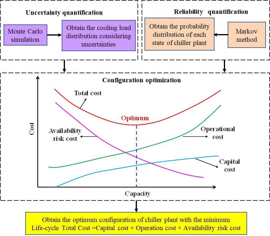
2.1. Outline of the Proposed Method

A chiller plant generally consists of several identical chillers (i.e., equal capacity) for the convenience of control and maintenance. However, a chiller plant consisting of chillers with different capacities can make the chiller plant work at a more efficient operating point, particularly at low part load conditions [39]. For instance, two chillers (rated cooling capacity of each chiller is 375 kW) provide cooling capacity for a commercial building (e.g., its peak cooling load is 750 kW). To supply 100 kW cooling capacity, the chiller operates at 26.7% of its rated cooling capacity, which is not within its efficient operating region (i.e., above 30%). When it is served by a big chiller (rated cooling capacity is 600 kW) and a small chiller (rated cooling capacity is 150 kW), the smaller chiller would operate at a very efficient operating point (i.e., 66.7% of its rated cooling capacity).

Our previous study [9] also showed that the optimum design of chiller plant should consist of several larger chillers and one smaller chiller based on the assumption that larger chillers usually have a higher COP (coefficient of performance) compared to smaller chillers. In operation, larger chillers generally operate at their highest efficient points with a nearly full load. When the total cooling load in operation is more than the total cooling capacity provided by all larger chillers, the smaller chiller would meet the rest cooling load and operate at a very efficient operating point.

The chiller plant generally works at part load conditions for a large proportion of the entire cooling season. Figure 1 presents typical COP curves of two types of chillers with constant-speed and variable-speed drivers, respectively. Constant-speed chillers have a higher operating COP when near the full load conditions compared to variable-speed chillers. On the contrary, when operating at part load conditions, especially low part load conditions, the variable-speed chillers perform much better.

In order to take both the uncertainty and reliability into account of the chiller plant design, the following assumptions are made:

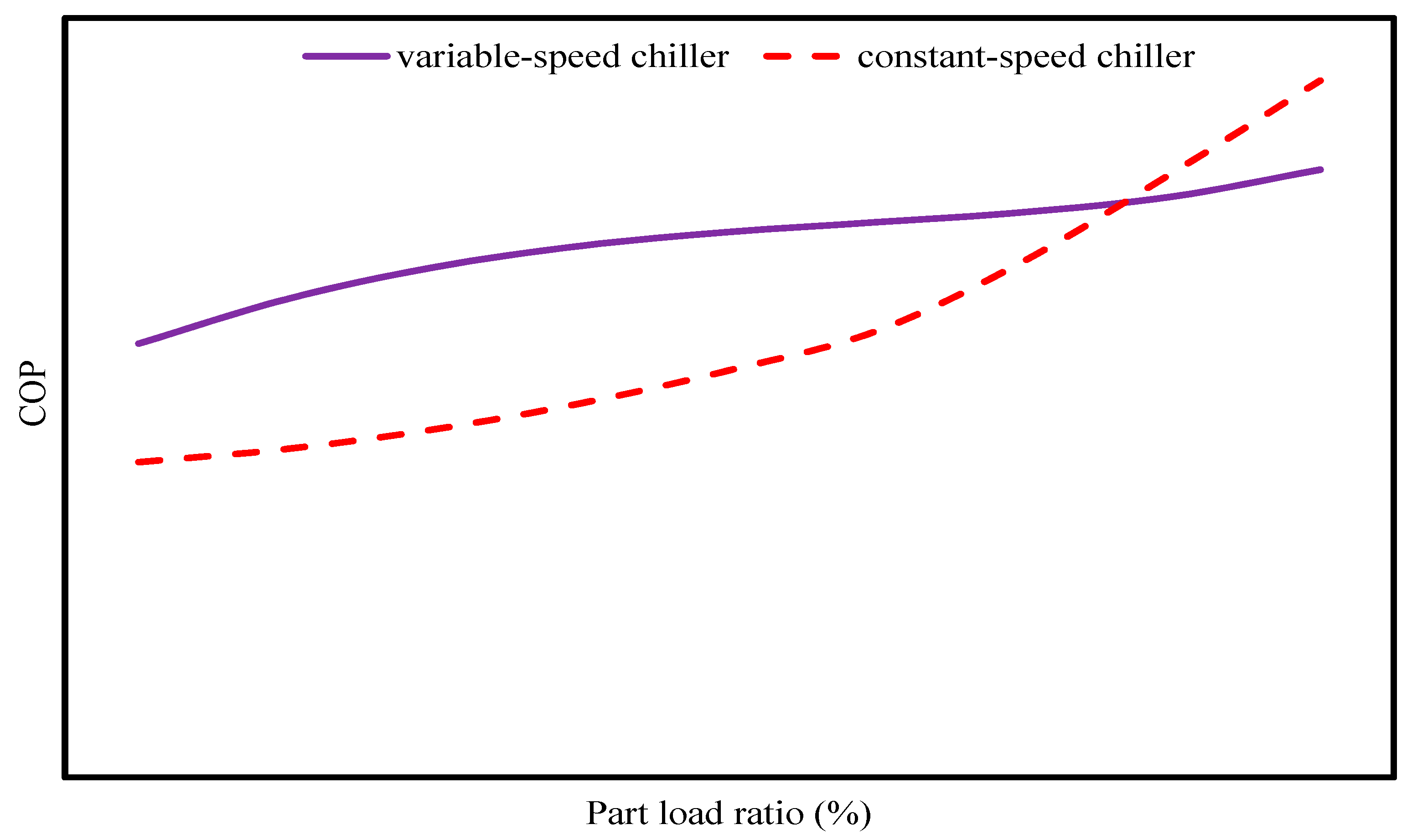
• A chiller plant consists of several constant-speed chillers, and no more than two variable-speed chillers.
• The failure rate of a constant-speed chiller is smaller than that of variable-speed chillers.
• All the constant-speed chillers are equally sized and have the same failure rate.
• All the variable-speed chillers are equally sized and have the same failure rate.

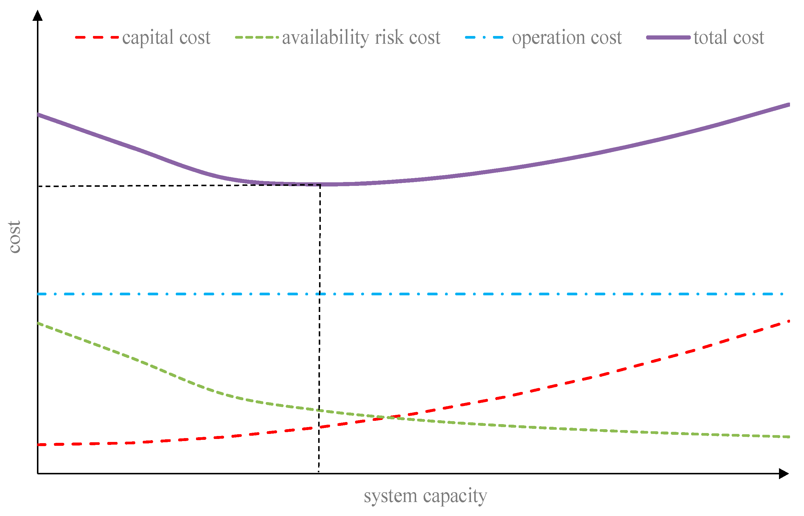
2.2. Objective of Design Optimization

The proposed design method aims at making sure that the sized chiller plant has enough capacity to supply sufficient cooling and to operate at its high efficient region under a large proportion of various cooling load conditions. Meanwhile, by considering both uncertainty and reliability, the annual total life-cycle cost for a chiller plant can approach the minimum value. In this study, the total cost (TC_n) is comprised of three aspects: (1) the capital cost (CC_n), (2) the operation cost (OC_n), and (3) the availability risk cost (RC_n) [8,9] (as shown in Equation (1)). Availability risk cost is a virtual “expense” for accounting the service sacrifice due to insufficient cooling supply [8]. A conceptual relationship between the total cooling capacity of a chiller plant and dedicated costs are illustrated in Figure 2. Generally, a larger cooling capacity means lower availability risk cost (e.g., higher reliability) and higher capital cost. Under the optimal configuration of a chiller plant (i.e., which make the chillers operate at efficient points as many times as possible), the operation cost maintains at a nearly constant value as the total cooling capacity increases. Referring to Figure 2, there is a comprised point, where the optimal total cooling capacity is identified when the minimum total cost is achieved.

$$T{C}_n=C{C}_n+O{C}_n+R{C}_n$$

(1)

3. Implementation of Robust Optimal Design for Chiller Plant Optimization

As shown in Figure 3, the optimal and robust design method is implemented according to the following four steps.

• Uncertainty quantification: Monte Carlo simulation is employed to obtain the cooling load distribution by considering the uncertainties of main design inputs;
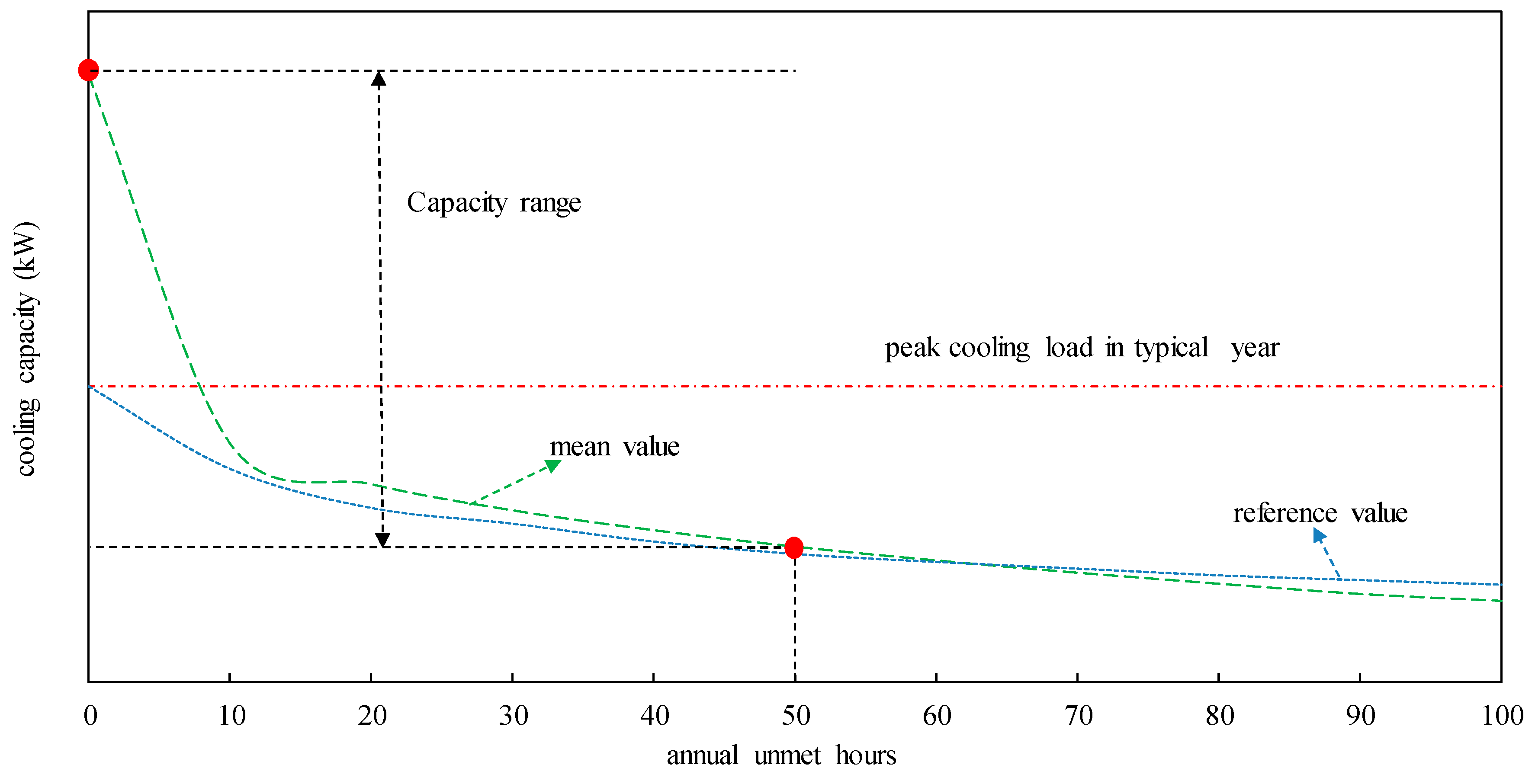
• Searching range quantification: the searching range of total chiller plant cooling capacity is specified according to the corresponding unmet hours in a cooling load distribution;
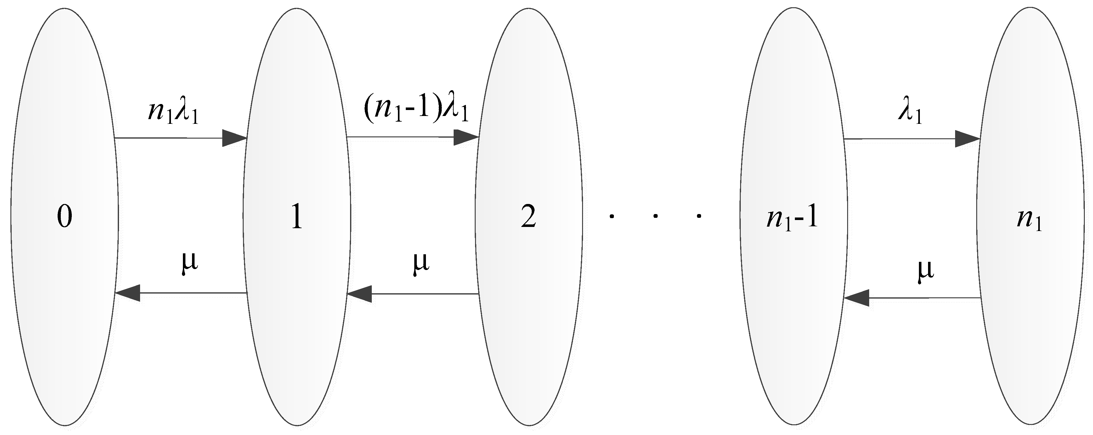
• Reliability quantification: Markov method is used to generate the probability distribution of various states of chiller plant by considering the failure rates of both constant-speed and variable-speed chillers;
• Chiller plant optimization: Trials of simulations focusing on the number/size of chillers and the sum of their cooling capacities to conduct trials on each total cooling capacity gradually, to obtain the total cost under various number/size of chillers on each total cooling capacity, and to obtain the optimal chiller plant option under each total cooling capacity.

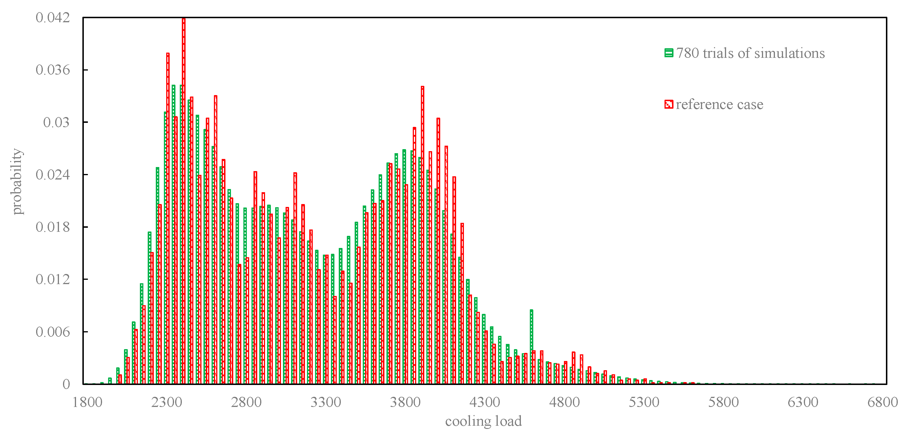
3.1. Quantification of Cooling Load Distribution Considering Uncertainties

The first step of using the proposed design method is to generate a representative distribution of a cooling load by sampling a large number of cooling load scenarios. In this paper, Monte Carlo simulation is selected to sample various scenarios for cooling load by considering uncertainties. The calculation process can be expressed using Equation (2). Y represents the calculated cooling load and the inputs x₁, x₂, …, x_n represent the inputs such as outdoor temperature, relative humidity, infiltration rate, etc. The quantification of uncertainties of inputs is conducted in MATLAB (Version 7.10.0, 2010, The MathWorks Inc, Natick, MA, USA). Based on such quantification results, the output y (i.e., cooling load scenario) is computed by the adoption of a Transient System Simulation (TRNSYS) building model. Generally, the uncertainties (e.g., outdoor temperature, relative humidity, fresh air rate, etc.) are represented by three typical distributions (e.g., uniform, tri-angular, and normal distributions) [8].

Table 1. Distributions of stochastic input parameters.

Parameters	Distributions
Outdoor temperature (°C) (T)	T × [1 + N(0, 1)]
Relative Humidity (%) (RH)	RH × [1 + N(0, 1.35)]
Number of Occupants (NO)	NO × T(0.3, 1.2, 0.9)
Fresh air rate (m3/person)	U(27, 33)
Light and equipment load (kW)	Design load × U(0.9, 1.1)

Remarks: N(µ, σ): normal distribution with mean value µ and standard deviation σ; U(a, b): uniform distribution between a and b; T (a, b, c): triangular distribution with lower limit a, upper limit b, and mode c.

shows a setting example of the input uncertainties [9]. In this table, the outdoor temperature and relative humidity are assumed to be normal distribution [8]. The outdoor temperature and relative humidity are within a reasonable range between the lowest temperature/relative humidity and highest temperature/relative humidity according to the statistical history data.

$$Y=f\left(x_1,x_2,\dots ,x_n\right)$$

(2)

It is worth noting that the quantification of uncertainties may have an important impact on the sizing of a chiller plant. If an alternative range of uncertainties is selected, the sized optimum chiller plant may change. The main focus of this study is on the process, development, and implementation of a new design method. However, the impact of quantification of uncertainties will not be discussed.

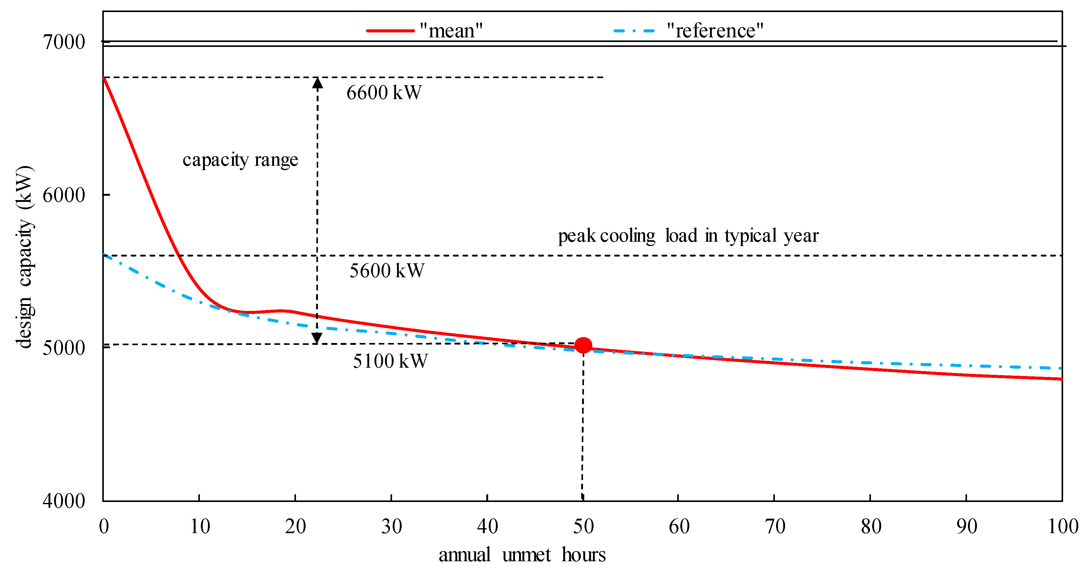
3.2. Quantification of Searching Range of Total Cooling Capacity

Specifying the searching range of total chiller plant cooling capacity is very important because it determines whether the sized chiller plant has the capacity to supply sufficient cooling. If an improper (e.g., overlarge in most cases) total cooling capacity is sized, the chiller plant may often operate within its low efficient region.

It is unreasonable to make a chiller plant always fulfill the cooling demand even under extreme conditions. Alternatively, the cooling capacities are usually determined based on the assumption that the selected cooling capacity may not fulfill the cooling demand within a certain value of unmet hours. In other words, the cooling demand under some adverse condition, whose appearance is regarded as a small probability event, can be considered as unmet. The value of unmet hours is therefore critical for identifying the searching range of total cooling capacity for a chiller plant. By considering uncertainties, the “mean” value symbolizes the cooling capacities corresponding to various unmet hours according to the cooling load distribution, as shown in Figure 4 [9]. The “reference” value symbolizes the cooling capacities according to the cooling load distribution in a typical year (i.e., TMY). In Figure 4, the peak value of a typical year is considered as a reference case to show the difference. The cooling capacities considering uncertainties are obviously lower than the peak value under several unmet hours. If the design capacity of the chiller plant is equal to the peak cooling load, the chiller plant operates within its low efficient region for a long time.

According to ASHRAE Standard 90.1, the total cooling capacity of a chiller plant should be the capacity corresponding to 50 unmet hours. For determining the searching range of cooling capacity, in this paper, the minimum cooling capacity is considered as the capacity corresponding to 50 unmet hours. The maximum cooling capacity is considered as the capacity fulfilling all the cooling load conditions including extreme conditions. An interval of each trial is 2.5% of the minimum cooling capacity.

3.3. Quantification of Probability Distribution of State for Chiller Plant

For the reliability assessment of multi-state systems, the Markov method is widely adopted [40]. In this paper, steady probability distribution of various states (e.g., fault state and fault-free state) for a chiller plant is generated by adopting the Markov method. Once probability distribution for each state is determined, the available capacity of a chiller plant can be estimated accordingly. The detailed assumptions of using the Markov method can be found in Reference [40].

The life-cycle of each component in this study contains operating period, maintenance period, and failure period. As shown in Equation (3), the MTTF (mean time to failure, 1/λ) represents the operating time. As shown in Equation (4), the MTTR (mean time to repair, 1/μ) is usually employed to represent the sum of maintenance time and failure time. Usually, the failure rate (λ) and the repair rate (μ) are employed as the major parameters for conducting the reliability assessment.

$$MTTF=\frac{1}{\lambda }$$

(3)

$$MTTR=\frac{1}{\mu }$$

(4)

Each chiller can be in two states: normal state (0) and failure state (1), which respectively represent when a chiller operates normally and abnormally. A chiller plant is assumed to consist of n₁ constant-speed chillers and n₂ variable-speed chillers. The constant-speed chillers have (n₁ + 1) states (i.e., each state includes several reliability scenarios) by accounting the reliability of constant-speed chillers as shown in Figure 5 [41]. As mentioned above, the number of variable-speed chillers is no more than two. As a result, the variable-speed chillers have three possible states (i.e., no chillers fail, one chiller fail, and two chillers fail). Totally, the chiller plant has 3(n₁ + 1) states, as shown in Equations (5–7). When only one variable-speed chiller is employed, p_2,n2 is equal to 0.

$$(p_{0,n_1}+p_{1,n_1}+\dots +p_{n_1-1,n_1}+p_{n_1,n_1})\cdot (p_{0,n_2}+p_{1,n_2}+p_{2,n_2})=1$$

(5)

$$p_{0,n_1}+p_{1,n_1}+\dots +p_{n_1-1,n_1}+p_{n_1,n_1}=1$$

(6)

$$p_{0,n_2}+p_{1,n_2}+p_{2,n_2}=1$$

(7)

The states of n₁ constant-speed chillers and the possible transitions among these different states are shown in Figure 5. There are totally (n₁ + 1) states, where the state 0 means that no constant-speed chillers failed and the state k means that there are k (1 ≤ k ≤ n) constant-speed chillers in failure. The chiller plant may transfer from one state to another due to failure and repair actions at a given period. As indicated by the arrows from left to right, the failure rate λ₁ equals the probability from one state in the left to the next adjacent state in the right. As indicated by the arrows from right to left, the repair rate μ equals the probability from one state in the right to the next adjacent state in the left. Herein, the term of “adjacent state” is used to describe two neighbor states. For example, “k + 1” state and “k − 1” state are two “adjacent states” of “k” state. As shown in Equation (8), the transition density matrix A represents the transition probability between any two adjacent states, which is corresponding to the failure and repair rates of constant-speed chillers. As shown in Equation (9), vector P(t) represents the probabilities of various states of constant-speed chillers at time t, which can be calculated by the derivation based on Equations (10) and (11). As shown in Equation (12), when the transition time accesses the infinity, the vector P(∞) will be constant. The probabilities of steady states are calculated by Equations (13) and (14).

$$A=\left[\begin{array}{cccccccc}(1-n_1{\lambda }_1)& n_1{\lambda }_1& 0& 0& 0\dots & 0& 0& 0\\ \mu & (1-\mu -(n_1-1){\lambda }_1)& (n_1-1){\lambda }_1& 0& 0\dots & 0& 0& 0\\ 0& \mu & (1-\mu -(n_1-2){\lambda }_1)& (n_1-2){\lambda }_1& 0\dots & 0& 0& 0\\ \dots & \dots & \dots & \dots & \dots & & & \\ 0& 0& 0& 0& 0\dots & \mu & (1-{\lambda }_1-\mu )& {\lambda }_1\\ 0& 0& 0& 0& 0\dots & 0& \mu & (1-\mu )\end{array}\right]$$

(8)

$$P(t)=\left[p_0(t),p_1(t),\dots ,p_n(t)\right]$$

(9)

$$P\left(0\right)=\left[1,0,0,\dots ,0\right]$$

(10)

$$P\left(n\right)=P(n-1)A=P\left(0\right)A^n$$

(11)

$$P(\infty )=\underset{\mathrm{n}\to \infty }{\lim }P(n)=\underset{\mathrm{n}\to \infty }{\lim }P\left(0\right)A^n$$

(12)

$$P(\infty )=P\left(\infty -1\right)A=P(\infty )A$$

(13)

$$\{\begin{array}{l}p(0)=a_{00}p(0)+a_{10}p(1)+\cdots +a_{n0}p(n)\\ p(1)=a_{01}p(0)+a_{11}p(1)+\cdots +a_{n1}p(n)\\ ⋮⋮\\ p(n)=a_{0n}p(0)+a_{1n}p(1)+\cdots a_{nn}p(n)\\ {\displaystyle \sum _{i=0}^{n}p(i)=1}\end{array}$$

(14)

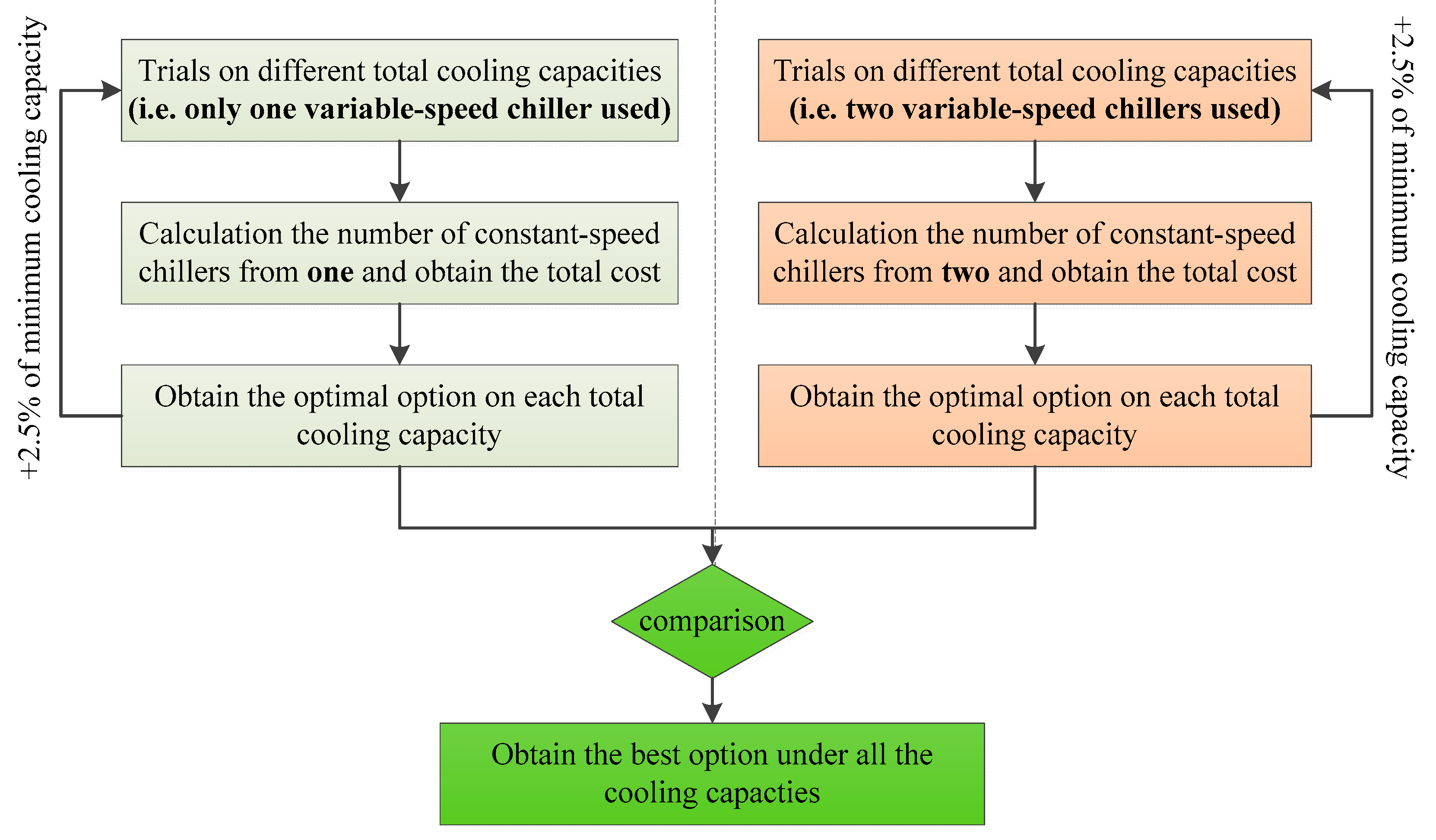
3.4. Optimization of the Configuration of Chiller Plant

In the previous design methods, optimization is often based on a given total cooling capacity (e.g., the cooling capacity corresponding to 50 unmet hours in the typical sample year). In this paper, the chiller plant configuration is optimized by comparing a series of total cooling capacities within a certain searching range. The optimized chiller plant could operate within a higher efficient region and have sufficient capacity to supply the cooling. By considering that chillers are manufactured in discrete size, trials on various total cooling capacities and discrete number/size of chillers are carried out to determine the optimum chiller plant configuration.

As mentioned above, the optimum chiller plant is selected based on the expected total cost. The most important part of total cost is the operating cost, which is mainly determined by the distribution of cooling load and energy efficiency of the chiller plant (i.e., COP). As shown in Equation (15), COP is mainly related to part load ratio (PLR) when the operating parameters, such as condensing temperature and evaporating temperature, are set to be constant.

$$CO{P}_i=D_0+D_1\cdot PL{R}_i+D_2\cdot PL{R}_i{}^2+D_3\cdot PL{R}_i{}^3$$

(15)

where, D₀–D₃ are the coefficients that can be fitted according to the chiller catalog or onsite measurement data. As shown in Equation (16), PLR is the ratio of operating cooling load (CL_opt) to the operating cooling capacity of chillers (CL_cc). Where, CL_rate is chiller rated capacity. N_op represents the number of chillers in operation.

$$PLR=\frac{C{L}_{opt}}{C{L}_{cc}}=\frac{C{L}_{opt}}{N_{op}\cdot C{L}_{rate}}$$

(16)

According to Equation (16), when the cooling load is given, the value of PLR is actually determined by the number of chillers in operation and the rated capacity. If more chillers are equipped (i.e., with larger flexibility to control the number of chillers in operation according to the actual cooling load to maximize the PLR), the actual operating PLR could be higher under proper sequence control strategies. Meanwhile, equipping more chillers indicates that the rated capacity of the individual chiller is smaller, which leads to the lower rated COP. Theoretically, an optimal value of chiller number exists when the highest operating COP is achieved. As shown in Figure 6 [42], once the operating chiller number approaches to a certain value, the operating COP can then achieve a higher level because the impact of increasing PLR is larger than that of decreasing rated COP. When the operating chiller number continually increases, the operating COP becomes lower because its PLR maintains at a nearly constant value and the rated COP reduces accordingly.

Figure 7 presents the implementation of simulation trials on each total cooling capacity to determine the optimum number and capacity of chillers. It contains two parts: (1) the trials under the condition that only one variable-speed chiller is employed; and (2) the trials under the condition that two variable-speed chillers are employed. For the trials under the condition that only one variable-speed chiller is employed, the numbers of constant-speed chillers are calculated starting from one until the operation cost starts to increase. In other words, at least two chillers are employed for system maintenance and reliability consideration. The option corresponding to the lowest total cost is selected from different cooling capacities. Equation (17) describes the sizing problem of a constant-speed chiller when only one variable-speed chiller is used.

$$\begin{array}{c}\mathrm{find}{C}_1,n_1,C_2\\ \mathrm{minimize}T{C}_{all}(C_1,n_1,C_2)\\ \mathrm{constraint}{n}_1{C}_1+C_2=C{L}_T\\ C_1>C_2,n_1\ge 1\end{array}$$

(17)

where C₁ represents capacity of constant-speed chiller, C₂ represents capacity of variable-speed chiller, TC represents total cost, and CL_T represents total cooling capacity.

For trials under the condition that two variable-speed chillers are employed, the number of constant-speed chillers are calculated starting from two until the operation cost starts to increase (i.e., the number of constant-speed chillers is not less than the number of variable-speed chillers). The option corresponding to the lowest total cost is also selected from different cooling capacities. Equation (18) describes the sizing problem of a constant-speed chiller when two variable-speed chillers are employed.

$$\begin{array}{c}\mathrm{find}{C}_1,n_1,C_2\\ \mathrm{minimize}T{C}_{all}(C_1,n_1,C_2)\\ \mathrm{constraint}{n}_1{C}_1+2C_2=C{L}_T\\ C_1>C_2,n_1\ge 2\end{array}$$

(18)

A comparison is made between the optimal configuration using one variable-speed chillers and the optimal configuration using two variable-speed chillers. Finally, configuration which gets the lowest total cost is considered as a better design.

4. Case Study and Discussion

A 50-storey office building in Hong Kong was chosen to demonstrate how to use the proposed design method for optimal sizing of a chiller plant. This building is a typical office with a total gross floor area of about 61,250 m². The design value for indoor air temperature and relative humidity are 25 °C and 50%, respectively. The lighting load and office equipment load are 10.8 W/m² and 8.1 W/m², respectively. The occupancy density is 18 m²/person and the fresh air rate is 30 m³/person. According to the proposed design method, the implementation process can be divided into four steps. Firstly, Monte Carlo simulation was employed to generate various sample scenarios for cooling load. Cooling load distribution with required accuracy can be also generated. Secondly, a searching range of total cooling capacity for a chiller plant was specified based on the cooling load distribution. Thirdly, by considering the failure rate difference between constant-speed and variable-speed chillers, a steady probability distribution for various states of a chiller plant was generated by the Markov method. Finally, trials on various total cooling capacities and discrete number/size of chillers were carried out to find the optimum chiller plant with the lowest total cost.

4.1. Cooling Load Distribution and Searching Range of Design Cooling Capacity

In order to generate a reasonable distribution of cooling load, before conducting the Monte Carlo simulations, it is necessary to quantify the uncertainties of input parameters. In this case study, the uncertainties of key inputs for cooling load calculation (including outdoor temperature, relative humidity, number of occupants, fresh air rate, lighting, and equipment load) are considered and their distributions are referred to in Table 1. Based on the quantification results of uncertainties from MATLAB, the cooling load scenarios are computed by the adoption of the TRNSYS building energy model. According to Reference [9], the sampling number of Monte Carlo simulation is set to be 780. Figure 8 shows the profiles of two types of cooling load distribution (i.e., the distribution of reference case, and distribution with considering uncertainties). In this paper, the distribution of reference case is a typical cooling load distribution of specified design year without considering uncertainties.

The next step is to find out the searching range of the total cooling capacity for a chiller plant. Various cooling capacities corresponding to different unmet hours are shown in Figure 9. The cooling capacities in the profile of “mean” are obviously larger than those in the profile of “reference” when the unmet hours are less than 10 hours, while such capacity differences become smaller gradually with the increase of the unmet hours. As defined, the maximum cooling load (i.e., 5600 kW) of a typical design year is higher than the minimum cooling capacity (i.e., around 5100 kW). When all the cooling load scenarios are fulfilled, the maximum cooling load is much smaller than the maximum cooling capacity (i.e., 6600 kW). The total cooling capacity searching range is between 5100 kW and 6600 kW and the interval is set to be 100 kW.

4.2. Probability Distribution of Chiller Plant State

In this study, the chiller plant is assumed to include 2~6 chillers totally. The failure rate of constant-speed chillers is assumed to be 0.0001/h and the failure rate of variable-speed chillers is assumed to be 0.000125/h. Both their repair rates are assumed to be 0.002/h [8,43].

The following step is to generate the steady probability distribution of a chiller plant under various numbers of variable-speed and constant-speed chillers. The chiller plant consists of one or two variable-speed chillers as mentioned. Referring to Equation (7), the probability distribution of variable-speed chillers can be obtained accordingly.

Table 2. Probability distribution of steady states of variable-speed chillers.

State	Variable-Speed Chillers
	1	2
0	0.9412	0.8828
1	0.0588	0.1103
2	-	0.0069

shows the steady probability distribution of various states of variable-speed chillers. The probability of state 0 is 0.9412 and the probability of state 1 is 0.0588, when only one variable-speed chiller is employed. The probabilities of state 0, 1, and 2 are 0.8828, 0.1103, and 0.0069, respectively, when two variable-speed chillers are employed. Referring to Equation (6), the probability distribution of constant-speed chillers can be obtained accordingly.

Table 3. Probability distribution of steady states of constant-speed chillers.

State	Number of Constant-Speed Chillers
	1	2	3	4	5
0	0.9524	0.9050	0. 8578	0.8109	0.7644
1	0.0476	0.0905	0.1278	0.1622	0.1911
2	-	0.0045	0.0129	0.0243	0.0382
3	-	-	0.0006	0.0024	0.0057
4	-	-	-	0.0001	0.0006
5	-	-	-	-	0

shows the steady probability distribution of various states for a different number of constant-speed chillers. It can be observed that the probability of state 0 decreases while the number of constant-speed chillers increases.

Referring to Equation (5), the probability distribution of the chiller plant can be obtained accordingly.

Table 4. An example of the probability distribution of a chiller plant.

Probability Distribution of Chiller Plant		State of Variable-Speed Chillers
		0	1	2
State of constant-speed chillers	0	0.67481	0.08431	0.00527
	1	0.16870	0.02108	0.00132
	2	0.03372	0.00421	0.00026
	3	0.00503	0.00063	0.00004
	4	0.00053	0.00007	0
	5	0	0	0

shows an example of the probability distribution of the chiller plant, which consists of two variable-speed chillers and five constant-speed chillers. This chiller plant gets 18 states totally (i.e., three states of variable-speed chillers and six states of constant-speed chillers). The probability of the chiller plant under the state 0 of variable-speed chillers and state 0 of constant-speed chillers is 0.67481, while the probability of the chiller plant under state 2 of variable-speed chillers and state 5 of constant-speed chillers is 0.

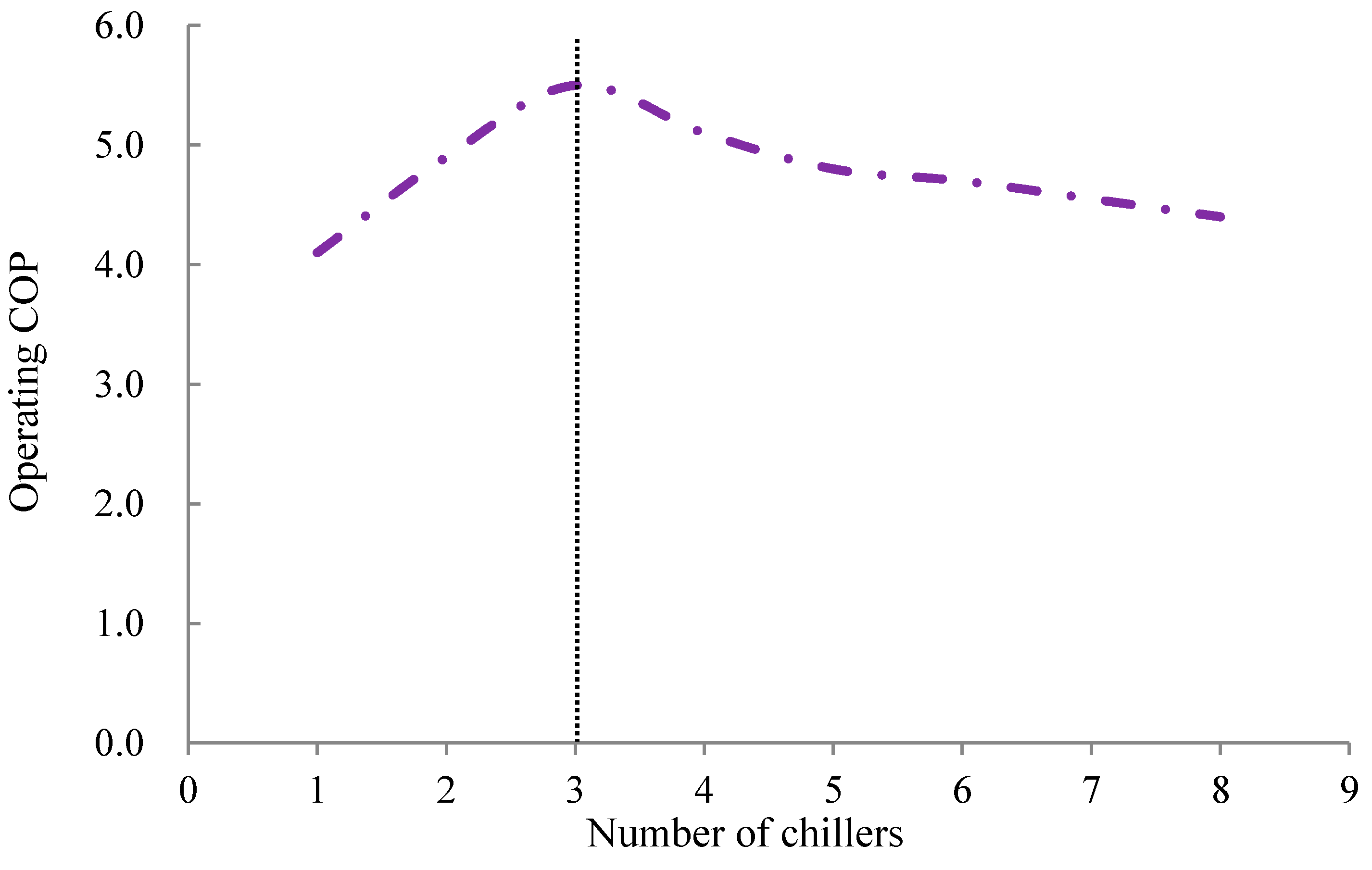
4.3. Tests on Total Cooling Capacity and Number/Size of Chillers

A total of 16 sets of simulation trials for the total cooling capacity were conducted between 5100 kW and 6600 kW, with a 100 kW searching interval, for instance, 5100 kW, 5200 kW,…, 6500 kW, and 6600 kW.

By taking the total cooling capacity of the chiller plant as 6000 kW for example, the operating COP increases with the chiller number increasing within a certain (i.e., 3 chillers) range, while the COP decreases when the chiller number further increases, as shown in Figure 6. By using the method as mentioned in Section 3.4, the operation cost of a chiller plant is estimated accordingly. Meanwhile, the rated cooling capacities of variable-speed and constant-speed chillers are optimized. The typical electricity price in Hong Kong is 1 HKD/kWh (note: 1 USD = 7.75 HKD). The operation cost of a chiller plant with different chiller combinations is presented in

Table 5. Annual operation cost and annualized capital cost of different design options.

Chiller Number	Chiller Plant Option (Size (kW) × Number)	Operation Cost (103 HKD)	Capital Cost (103 HKD)
2	3200 × 1CSD + 2800 × 1VSD	3502	373
3	2100 × 2CSD + 1800 × 1VSD	3478	461
4	1550 × 3CSD + 1350 × 1VSD	3461	542
4	1600 × 2CSD + 1400 × 2VSD	3446	580
5	1250 × 4CSD + 1000 × 1VSD	3436	616
5	1300 × 3CSD + 1050 × 2VSD	3403	653
6	1050 × 5CSD + 750 × 1VSD	3435	685
6	1050 × 4CSD + 900 × 2VSD	3392	723

Remarks: CSD: constant-speed chiller, VSD: variable-speed chiller.

. Generally, the chiller plant operation cost of two variable-speed chillers is lower than that of one variable-speed chiller. Among all the selected combinations, the design option consisting of two variable-speed chillers (900 kW cooling capacity) and four constant-speed chillers (1050 kW cooling capacity) gets the minimum operation cost.

The capital cost mainly includes the space cost and the equipment cost. The chiller plant lifespan is assumed to be 10 years in this case study. The space costs for variable-speed and constant-speed chillers are assumed to be 20,000 HKD and 15,000 HKD, respectively. The equipment costs of constant-speed and variable-speed chillers (rated cooling capacities of these two types of chillers are the same here: 900 kW) are 0.9 MHKD and 1.2 MHKD, respectively, by referring to manufacture data. The equipment costs (EC) of chillers with other capacities can be calculated according to Equation (19) [44,45].

$$EC=E{C}_0\cdot {\left(C/C_0\right)}^{\alpha }$$

(19)

where, EC₀ is the reference equipment cost of a specific chiller capacity C₀. EC is the equipment cost of chiller capacity C. α is a coefficient and its value is determined as 0.15 according to [46]. The annualized capital cost is calculated as the sum of space cost and equipment cost divided by the lifespan (10 years), and the results are shown in Table 5.

The availability risk cost means a virtual “penalty expense” (i.e., so called “service sacrifice”) when cooling demands cannot be satisfied due to insufficient cooling supply (e.g., equipment failures), which can be calculated according to the unmet demand and the assumed penalty ratios.

Table 6. Annual availability risk cost (10³ HKD) and total cost (10³ HKD) of different design options.

Penalty Ratio (HKD/kW)	1		10		100
Option (Size(kW) × Number)	RC	TC	RC	TC	RC	TC
3200 × 1CSD + 2800 × 1VSD	102	3978	1021	4897	10,210	14,085
2100 × 2CSD + 1800 × 1VSD	39	3977	387	4326	3871	7810
1550 × 3CSD + 1350 × 1VSD	25	4140	247	4362	2468	6583
1600 × 2CSD + 1400 × 2VSD	25	4053	254	4282	2542	6570
1250 × 4CSD + 1000 × 1VSD	19	4070	185	4237	1851	5903
1300 × 3CSD + 1050 × 2VSD	28	4084	275	4331	2755	6811
1050 × 5CSD + 750 × 1VSD	15	4135	145	4265	1451	5571
1050 × 4CSD + 900 × 2VSD	22	4165	216	4331	2161	6276

Remarks: RC: availability risk cost, TC: total cost.

shows the total costs and the availability risk costs for different design options when there are three levels of penalty ratios (i.e., 1 HKD/kW, 10 HKD/kW, and 100 HKD/kW). The availability risk cost rapidly decreases with the increasing of the chiller number when the number is small. The total cost decreases when the chiller number increases. Since the availability risk cost is high with a small chiller number, while the capital cost is high with a big chiller number, there is a comprised configuration of chiller numbers/sizes with the lowest total cost. In this paper, the penalty ratio is set to be 10 HKD/kW. In all these options, the combination with one variable-speed chiller (1000 kW cooling capacity) and four constant-speed chillers (1250 kW cooling capacity) gets the lowest total cost 4237 × 10³ HKD, which has good robustness subject to uncertainties and reliability. It is therefore considered to be the best configuration corresponding to the total cooling capacity 6000 kW. If the penalty ratio is set to be 1 HKD/kW, the best configuration corresponding for the total cooling capacity is one variable-speed chiller (1800 kW cooling capacity) and two constant-speed chillers (2100 kW cooling capacity). Designers should select the best configuration according to the level of penalty.

Table 7. Best design options under different total cooling capacities (penalty ratio: 10 HKD/kW).

Total Cooling Capacity (kW)	Best Option (Size (kW) × Number)	Availability Risk Cost (103 HKD)	Operation Cost (103 HKD)	Total Cost (103 HKD)
5100	1050 × 4CSD + 900 × 1VSD	490	3397	4469
5400	1100 × 4CSD + 1000 × 1VSD	343	3412	4350
5700	1150 × 4CSD + 1100 × 1VSD	246	3421	4274
6000	1250 × 4CSD + 1100 × 1VSD	185	3436	4237
6300	1300 × 4CSD + 1100 × 1VSD	131	3463	4222
6600	2300 × 2CSD + 2000 × 1VSD	253	3501	4231

summarizes the calculation results of lowest total costs corresponding to different total cooling capacities. When the total chiller plant cooling capacity increases from 5100 kW to 6300 kW, the total costs reduce due to the rapid decrease of availability risk costs when the optimal combination is identified. However, the total cost increases when the total cooling capacity is over 6300 kW. Compared with other options, results show that the combination with one variable-speed chiller (1100 kW cooling capacity) and four constant-speed chillers (1300 kW cooling capacity) achieves the lowest total cost 4222 × 10³ HKD. The major reason for achieving such a result is attributed to the lowest availability risk cost as a better robustness for uncertainties, and system reliability can be achieved by the selected option.

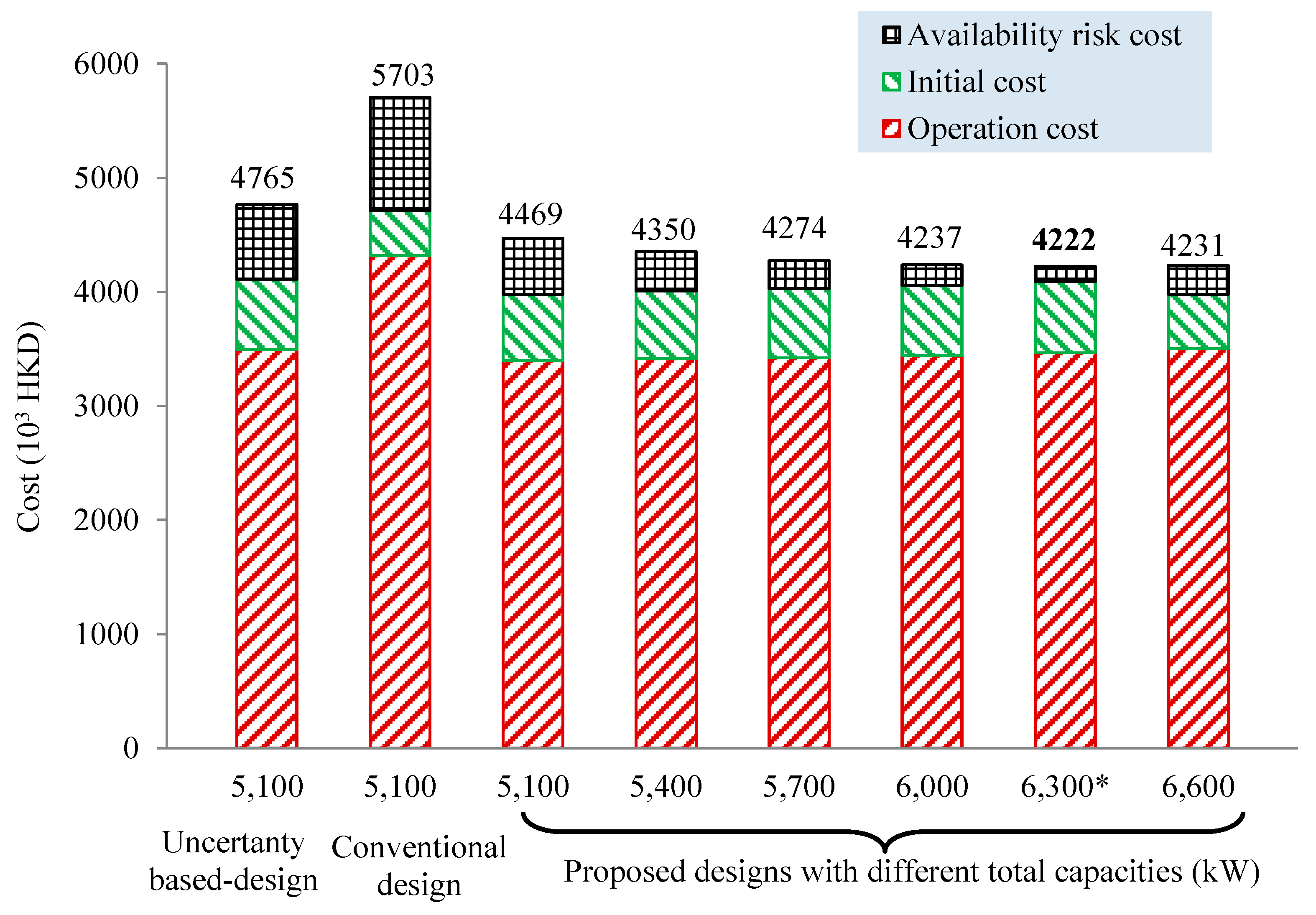
4.4. Comparison among Different Configurations Using Design Methods

Table 8. Optimal configurations using different design methods (penalty ratio: 10 HKD/kW).

	Total Cooling Capacity (kW)	Best Configuration (Size (kW) × Number)	Availability Risk Cost (103 HKD)	Operation Cost (103 HKD)	Total Cost (103 HKD)
Robust optimal design	6300	1300 × 4CSD + 1100 × 1VSD	131	3463	4222
Uncertainty-based design	5100	1400 × 3CSD + 900 × 1VSD	656	3495	4765
Conventional design	5100	1700 × 3CSD	992	4318	5703

compares the design results from three different design methods: (1) the robust optimal design, (2) the uncertainty-based design (i.e., developed in Reference [9]), and (3) the conventional design. The combination with one variable-speed chiller (1100 kW cooling capacity) and four constant-speed chillers (1300 kW cooling capacity) is selected as the optimal design to achieve the lowest annual total cost. By comparing with uncertainty-based and conventional designs, the total cost of robust optimal design (4222 × 10³ HKD) is reduced about 26% and 11.4%, respectively, when the penalty ratio is 10 HKD/kW. To better demonstrate the impact of different design methods and configurations on design results, the operation cost, initial cost, and availability risk cost of eight optimum design options are shown in Figure 10. Among these eight design options, six options are using robust optimal design method with different total capacities. It can be observed that the total costs of six robust optimal design options are obviously lower than that of uncertainty-based and conventional design methods while the total cost differences among the six robust optimal design options are not significant. This indicates that the proposed design method can provide a more robust and more cost-effective design option than existing design methods.

5. Conclusions

This paper presents a novel optimal design method for a chiller plant based on life-cycle total cost optimization. By quantitatively considering the uncertainties of design inputs and the reliabilities of equipment in operation for a chiller plant, the proposed method can ensure a high energy efficiency and sufficient cooling supply under various cooling load scenarios. Minimized life-cycle total cost can be achieved by optimizing the total cooling capacity and the configurations of a chiller plant (i.e., numbers/sizes of chillers). A case study has also been conducted to validate the proposed method. The main conclusions are drawn as follows:

• The searching range of total cooling capacity of a chiller plant can be determined by the cooling capacities with predefined unmet hours under the cooling load distribution. In the case study, the minimum cooling capacity is 5100 kW and the maximum cooling capacity is 6600 kW.
• Although the chiller plant with one variable-speed chiller might operate at a lower efficiency than that with two variable-speed chillers, the design option with one variable-speed chiller is still more economical when the life-cycle total cost is considered.
• The design option of a chiller plant using the proposed method can operate with a relatively high efficiency, and has a relatively sufficient cooling capacity to supply the cooling under various cooling load scenarios. The lowest total cost can be achieved by considering both design uncertainties and reliabilities for a chiller plant.
• Results show that the life-cycle total cost of optimal and robust design is reduced by 26% and 11.4%, respectively, when compared with those from uncertainty-based and conventional design methods.

References

1. EMSD Hong Kong Energy End-Use Data. Available online: https://www.emsd.gov.hk/filemanager/en/content_762/HKEEUD2012.pdf (accessed on 12 April 2019).
2. Sun, Y.J.; Wang, S.W.; Xiao, F. In situ performance comparison and evaluation of three chiller sequencing control strategies in a super high-rise building. Energy Build. 2013, 61, 333–343. [Google Scholar] [CrossRef]
3. Lee, W.L.; Yik FW, H.; Jones, P. Energy saving by realistic design data for commercial buildings in Hong Kong. Appl. Energy 2001, 70, 59–75. [Google Scholar]
4. ASHRAE Handbook—HVAC Systems and Equipment; ASHRAE: Atlanta, GA, USA, 2012.
5. Rudoy, W.; Cuba, J.F. Cooling and Heating Load Calculation Manual; ASHRAE: Atlanta, GA, USA, 1979. [Google Scholar]
6. EnergyPlus energy simulation software, 2015.
7. TRNSYS. TRNSYS 16 Documentation. 2004. Available online: http://sel.me.wisc.edu/trnsys (accessed on 12 April 2019).
8. Cheng, Q.; Wang, S.; Yan, C. Robust optimal design of chilled water systems in buildings with quantified uncertainty and reliability for minimized life-cycle cost. Energy Build. 2016, 126, 159–169. [Google Scholar] [CrossRef]
9. Cheng, Q.; Wang, S.; Yan, C.; Xiao, F. Probabilistic approach for uncertainty-based optimal design of chiller plants in buildings. Appl. Energy 2017, 185, 1613–1624. [Google Scholar] [CrossRef]
10. Domínguez-Muñoz, F.; Cejudo-López, J.M.; Carrillo-Andrés, A. Uncertainty in peak cooling load calculations. Energy Build. 2010, 42, 1010–1018. [Google Scholar] [CrossRef]
11. Sun, Y.; Gu, L.; Wu, C.F. Exploring HVAC system sizing under uncertainty. Energy Build. 2014, 81, 243–252. [Google Scholar] [CrossRef]
12. Yik, F.W.H.; Lee, W.L.; Burnett, J. Chiller plant sizing by cooling load simulation as a means to avoid oversized plant. HKIE Trans. 1999, 6, 19–25. [Google Scholar] [CrossRef]
13. Djunaedy, E.; Van Den Wymelenberg, K.; Acker, B.; Thimmana, H. Oversizing of HVAC system: Signatures and penalties. Energy Build. 2011, 43, 468–475. [Google Scholar] [CrossRef]
14. Woradechjumroen, D.; Yu, Y.; Li, H.; Yu, D.; Yang, H. Analysis of HVAC system oversizing in commercial buildings through field measurements. Energy Build. 2014, 69, 131–143. [Google Scholar]
15. Braun, J.E.; Klein, S.A.; Mitcelj, W. Applications of optimal control to chilled water systems without storage. ASHRAE Trans. 1989, 95, 663–675. [Google Scholar]
16. Gidwani, B.N. Optimization of chilled water systems. Energy Eng. 1987, 84, 83–91. [Google Scholar]
17. Kaya, A. Improving efficiency in existing chillers with optimization technology. ASHRAE J. 1991, 33, 30–38. [Google Scholar]
18. Chang, Y.C.; Lin, J.K.; Chuang, M.H. Optimal chiller loading by genetic algorithm for reducing energy consumption. Energy Build. 2005, 37, 147–155. [Google Scholar] [CrossRef]
19. Yu, F.W.; Chan, K.T. Strategy for designing more energy efficient chiller plants serving air-conditioned buildings. Build. Environ. 2007, 42, 3737–3746. [Google Scholar] [CrossRef]
20. Hartman, T. All-variable speed centrifugal chiller plants. ASHRAE J. 2001, 43, 43–53. [Google Scholar]
21. Celuch, J. Hybrid chilled water plant. ASHRAE J. 2001, 43, 34–35. [Google Scholar]
22. Ashouri, A.; Petrini, F.; Bornatico, R.; Ben, M.J. Sensitivity analysis for robust design of building energy systems. Energy 2014, 76, 264–275. [Google Scholar] [CrossRef]
23. Van Gelder, L.; Janssen, H.; Roels, S. Effective and robust measures for energy efficient dwellings: Probabilistic determination. Build. Simul. 2013, 2013, 3465–3472. [Google Scholar]
24. Fiksel, J. Designing resilient, sustainable systems. Environ. Sci. Technol. 2003, 37, 5330–5339. [Google Scholar] [CrossRef]
25. Morari, M. Flexibility and resiliency of process systems. Comput. Chem. Eng. 1983, 7, 423–437. [Google Scholar] [CrossRef]
26. Pettersen, T.D. Variation of energy consumption in dwellings due to climate, building and inhabitants. Energy Build. 1994, 21, 209–218. [Google Scholar] [CrossRef]
27. Li, C.Z.; Shi, Y.M.; Huang, X.H. Sensitivity analysis of energy demands on performance of CCHP system. Energy Convers. Manage. 2008, 49, 3491–3497. [Google Scholar] [CrossRef]
28. Smith, A.; Luck, R.; Mago, P.J. Analysis of a combined cooling, heating, and power system model under different operating strategies with input and model data uncertainty. Energy Build. 2010, 42, 2231–2240. [Google Scholar] [CrossRef]
29. Menassa, C.C. Evaluating sustainable retrofits in existing buildings under uncertainty. Energy Build. 2011, 43, 3576–3583. [Google Scholar] [CrossRef]
30. Stapelberg, R.F. Handbook of Reliability, Availability, Maintainability and Safety in Engineering Design; Springer: London, UK, 2009. [Google Scholar]
31. Vanderhaegen, F.A. Non-probabilistic prospective and retrospective human reliability analysis method—Application to railway system. Reliab. Eng. Syst. Safe. 2001, 71, 1–13. [Google Scholar] [CrossRef]
32. Peruzzi, L.; Salata, F.; De Lieto Vollaro, A.; De Lieto Vollaro, R. The reliability of technological systems with high energy efficiency in residential buildings. Energy Build. 2014, 68, 19–24. [Google Scholar] [CrossRef]
33. Au-Yong, C.P.; Ali, A.S.; Ahmad, F. Improving occupants’ satisfaction with effective maintenance management of HVAC system in office buildings. Automat. Constr. 2014, 43, 31–37. [Google Scholar] [CrossRef]
34. Kwak, R.Y.; Takakusagi, A.; Sohn, J.Y.; Fujii, S.; Park, B.Y. Development of an optimal preventive maintenance model based on the reliability assessment for air-conditioning facilities in office buildings. Build. Environ. 2004, 39, 1141–1156. [Google Scholar] [CrossRef]
35. Cheng, Q.; Wang, S.; Yan, C. Sequential Monte Carlo Simulation for Robust Optimal Design of Cooling Water System with Quantified Uncertainty and Reliability. Energy 2017, 118, 489–501. [Google Scholar] [CrossRef]
36. Esen, H.; Inalli, M.; Esen, M. Technoeconomic appraisal of a ground source heat pump system for a heating season in eastern Turkey. Energy Convers. Manage. 2006, 47, 1281–1297. [Google Scholar] [CrossRef]
37. Esen, H.; Inalli, M.; Esen, M. A techno-economic comparison of ground-coupled and air-coupled heat pump system for space cooling. Build. Environ. 2007, 42, 1955–1965. [Google Scholar] [CrossRef]
38. Esen, M.; Yuksel, T. Experimental evaluation of using various renewable energy sources for heating a greenhouse. Energy Build. 2013, 65, 340–351. [Google Scholar] [CrossRef]
39. Stanford, H.W., III. HVAC Water Chillers and Cooling Towers: Fundamentals, Application, and Operation; CRC Press: Boca Raton, FL, USA, 2011. [Google Scholar]
40. Lisnianski, A.; Levitin, G. Multi-State System Reliability: Assessment, Optimization and Applications; World Scientific: Singapore, 2003. [Google Scholar]
41. Lisnianski, A. Extended block diagram method for a multi-state system reliability assessment. Reliab. Eng. Syst. Safe. 2007, 92, 1601–1607. [Google Scholar] [CrossRef]
42. Harvey, D. A Handbook on Low-Energy Buildings and District-Energy Systems: Fundamentals, Techniques and Examples; Routledge: Abingdon, UK, 2012. [Google Scholar]
43. Blanchard, A.; Roy, B.N. Savannah River Site Generic Data Base Development; WSRC-TR-93-262, REV.1; Westinghouse Safety Management: Aiken, SC, USA, 1998. [Google Scholar]
44. Guthrie, K.M. Capital cost estimating. Chem. Eng. 1969, 3, 114–142. [Google Scholar]
45. Biegler, L.T.; Grossmann, I.E.; Westerberg, A.W. Systematic Methods for Chemical Process Design; Prentice Hall PTR: Upper Saddle River, NJ, USA, 1997. [Google Scholar]
46. Taal, M.; Bulatov, I.; Klemeš, J.; StehlíK, P. Cost estimation and energy price forecasts for economic evaluation of retrofit projects. Appl. Therm. Eng. 2003, 23, 1819–1835. [Google Scholar] [CrossRef]
Figure 1. Coefficient of performance (COP) of a constant-speed chiller and a variable-speed chiller.
Applsci 09 01548 g001
Figure 2. Total cost vs. total cooling capacity.
Applsci 09 01548 g002
Figure 3. Procedure of the proposed robust optimal design.
Applsci 09 01548 g003
Figure 4. Cooling capacity vs. unmet hours.
Applsci 09 01548 g004
Figure 5. States of n1 constant-speed chillers and possible transitions.
Applsci 09 01548 g005
Figure 6. COP vs. number of chillers.
Applsci 09 01548 g006
Figure 7. Trials of simulation to select optimum chiller plant design.
Applsci 09 01548 g007
Figure 8. Distribution of cooling load with and without considering uncertainties.
Applsci 09 01548 g008
Figure 9. Cooling capacities vs. number of annual unmet hours.
Applsci 09 01548 g009
Figure 10. The costs of the optimum configurations using different design methods.
Applsci 09 01548 g010