Image Recovery with Data Missing in the Presence of Salt-and-Pepper Noise

Abstract

In this paper, an image recovery problem under the case of salt-and-pepper noise and data missing that degrade image quality is addressed if they are not effectively handled, where the salt-and-pepper noise as the impulsive noise is remodeled as a sparse signal due to its impulsiveness and the data missing pattern, denoted by a sparse vector, contains only zeros and ones to formulate the data missing. In particular, the salt-and-pepper noise and data missing are reformatted by their sparsity, respectively. The wavelet and framelet domains are explored to sparsely represent the image in order to accurately reconstruct the clean image. From the reformulations conducted and to recover the image, under one optimization framework, a joint estimation is developed to perform the image recovery, the salt-and-pepper noise suppression, and the missing patter estimation. To solve the optimization problem, two efficient solvers are developed to obtain the joint estimation solution, and they are based on the alternating direction method of multipliers (ADMM) and accelerated proximal gradient (APG). Finally, numerical studies verify that the joint estimation algorithm outperforms the state-of-the-art approaches in terms of both objective and subjective evaluation standards.

1. Introduction

Image restoration is an important and widely studied subject in image processing, where the main objective is to reconstruct the latent image given the degraded and/or noisy image [1,2,3,4,5]. The main detrimental factors to corrupt the image are noise, data missing, and blur, to name a few. It is well known that images are deteriorated if they are not properly handled, and, in this work, the image restoration approach is developed when the image is corrupted by salt-and-pepper noise and data  missing.

The salt-and-pepper noise, classified as the impulsive noise, presents a great challenge for an image reconstruction problem because of its impulsive nature. The noise is mainly caused by imaging sensors, transmissions, and/or other factors. Under the case of salt-and-pepper noise, the approaches developed for Gaussian noise will not work well because the noise distributions are different. To suppress the noise, the traditional techniques mainly focus on filters in which nonlinear filters and linear filters are developed. In contrast, nonlinear filters in general offer better performance than linear filters. The classical nonlinear filter in the context of impulsive noise removal is the standard median (MED) filter [6]. It can easily be shown that this type of filter is conceptually simple to implement and hence provides good denoising ability, but its performance deuterates as the noise level increases. Shortly after, the detection-removing approaches are then devised so as to better suppress the noise, where the noisy pixels are detected first, and second they are replaced by the results of a certain type of median filters using vicinity pixels—for example, the adaptive median filter (AMF) [7] and its improved versions of adaptive weighted mean filter (AWMF) [8,9], the multistate median (MSM) filter [10] and the adaptive median filter with edge-preserving regularization (AM-IEPR) [11]. Computer simulation results show that the above-mentioned filters outperform the traditional MED filter, but their performance largely depends on the performance of the detection. The main drawback of these approaches is that they failed to exploit the noise structure that might improve the noise suppression ability and in turn enhance the image reconstruction.

In practice, data missing happens because of sensor failure and sudden data transmission loss. Over the past several decades, a huge number of approaches have been proposed to handle this issue. Based on the structural inpainting technique, several algorithms were reported for accurate reconstruction of missing edges, and they are effective for pure structure images [12,13]. However, for images containing textures, the performances were less satisfactory. To remedy this issue, the exemplar-based inpainting technique was exploited to develop several methods for accurate reconstruction of missing textures [4,14,15,16]. Traditionally, missing texture reconstruction is considered as the texture synthesis, and, based on which, many methods were proposed—for example, the fragment-based algorithm [14] and the exemplar-based image inpainting method [15]. In [16], the approach for learning a high-order Markov random field (MRF) has been proposed and the performance of missing texture reconstruction is dramatically improved. The key idea is to formulate the prior as a high-order Markov random field (MRF) defined over large neighborhood systems. By decomposing the exemplars into the frequency domain and using the selected coefficients, the gradient based algorithm was developed to interpolate the missing parts, and its superior performance was demonstrated because the coefficient selection process acts to remove the noise [17,18]. Recently, due to the successful developments of the sparse signal reconstruction, many methods have been proposed by exploiting the sparse representation of the image [4,19,20,21]. Even they provide better reconstruction results in some cases, the performance degrades when the missing level is high.

To handle those issues, namely salt-and-pepper noise and data missing, in this paper, a joint estimation approach is developed to simultaneously recover the image and missing pattern under the salt-and-pepper noise condition. The primary objective of this work focuses on utilizing a sparse property of signals. To explore the sparse property of images, two representative domains, namely wavelet and framelet domains, are introduced in which the natural images have a sparse representation. Thanks to the impulsive nature of the noise, its sparsity is also observed in the time domain since it contains few nonzero values and lots of zero values. Therefore, the noise suppression becomes a parameter estimation problem, where the noise is actively reduced rather than passively being suppressed. To reveal the sparse property of the missing pattern, a vector that consists of only zeros and ones is introduced to remodel the missing measurements problem in which the element is one if the measurement is received correctly and zero if the corresponding measurement is missed. With the reformulations introduced, a joint optimization framework is readily developed to perform image and missing pattern estimation while suppressing the salt-and-pepper noise. A two-step iterative approach is proposed in order to efficiently solve this optimization problem, where each step contains a convex optimization problem. At every step, the resultant problem is an ${\ell }_1$-norm constrained optimization, and two algorithms, called ADMM and APG, are tailored to solve the optimization problems. To demonstrate the performance of the proposed joint estimation approach, experiments in three situations such as salt-and-pepper noise only, data missing only, and the combination of salt-and-pepper noise and data missing are respectively conducted. The main difference compared to the work presented in [1] is that the data missing issue is addressed instead of the deblur problem.

The rest of the paper is organized as follows: the formulations of the salt-and-pepper noise and data missing are presented in Section 2. In Section 3, two sparse transform domains, namely wavelet and framelet are briefly introduced. A joint estimation is provided that utilizes the sparse properties of salt-and-pepper noise, data missing and image to perform the noise suppression, missing pattern estimation, and image recovery in Section 4. To efficiently obtain the solution, two solvers based on ADMM and APG are developed. In Section 5, numerical studies for the proposed approach are presented. Finally, this paper concludes with a brief summary in Section 6.

2. Formulations of Salt-and-Pepper Noise and Data Missing

In this work, the degraded image is given by

$$\begin{array}{c}\hfill \begin{array}{c}\hfill \mathbf{y}=\mathbf{H}\mathbf{x}+\mathbf{n},\end{array}\end{array}$$

(1)

where $\mathbf{y}$ is the degraded image, $\mathbf{x}$ is the latent image to be reconstructed, $\mathbf{H}$ is the degradation matrix, and $\mathbf{n}$ is the noise. It is of interest to note that the column representation of the image is used in Equation $(1)$.

For a pure denoising problem, the degradation matrix is usually an identity matrix and the noise $\mathbf{n}$ is the main source of interference. The noise can be generally divided into two categories: Gaussian noise and impulsive noise. It is a consensus that the impulsive noise is much harder to be removed than the Gaussian noise, and, in this work, one type of the impulsive noise salt-and-pepper noise is considered. The clean image is corrupted by the salt-and-pepper noise. That is,

$$\begin{array}{cc}\hfill y(i)& =\left\{\begin{array}{cc}{n}_{min},& \mathrm{with}\mathrm{probability}p/2,\hfill \\ n_{max},& \mathrm{with}\mathrm{probability}p/2,\hfill \\ x(i),& \mathrm{with}\mathrm{probability}1-p,\hfill \end{array}\right.\hfill \end{array}$$

(2)

where p denotes the probability, $n_{min}$ and $n_{max}$ indicate the minimum and maximum values of the dynamic range, and they are 0 and 255 for a grey image, respectively. In Equation $(2)$, one important observation is that only $p\times 100\%$ pixels are affected by the noise and the rest is not. This is to say that, if the additive noise model in Equation $(1)$ is used, the noise $\mathbf{n}$ has lots of zero components. Therefore, $\mathbf{n}$ can be seen as a sparse vector and this property will be exploited to remove the noise. For more information, the readers are referred to [22].

Another detrimental factor for image reconstruction is data missing due to the unreliable transmission link and/or other reasons. When this happens, the corresponding pixel is set to be zero and the rest is unchanged. In doing so, a sparse vector can be introduced to reformulate the data missing signal model. For example, let the uniform samples be ${[y_1,y_2,y_3,y_4]}^{\mathrm{T}}$, and suppose the pixels of $y_1,y_2$ are missing. The received signal that contains samples of $y_3,y_4$ is modeled as ${[y_3,y_4]}^{\mathrm{T}}=\mathbf{H}\circ {[y_1,y_2,y_3,y_4]}^{\mathrm{T}}$, where $\mathbf{H}={[0,0,1,1]}^{\mathrm{T}}$ and ∘ is Hadamard product to indicate a componentwise product. In this reformulation, an unknown sparse vector $\mathbf{H}$ is introduced to model the data missing pattern and it will be utilized to estimate the missing pattern. To simplify the following derivations, the missing pattern is rewritten in a matrix form, denoted by $\mathbf{H}$. By using the matrix notation, the missing pattern in this example is a sparse matrix; that is, $\mathbf{H}=[0010;0001]$. With this reformulation, in the case of data missing, the received signal is [23]

$$\begin{array}{c}\hfill \begin{array}{c}\hfill \tilde{\mathbf{y}}=\mathbf{H}\mathbf{y}=\mathbf{H}(\mathbf{x}+\mathbf{n})=\mathbf{H}\mathbf{x}+\tilde{\mathbf{n}},\end{array}\end{array}$$

(3)

where $\tilde{\mathbf{y}}$ is the received signal in the case of data missing, $\mathbf{H}$ is the unknown missing pattern, and $\tilde{\mathbf{n}}$ is the salt-and-pepper noise.

If we now wish to recover the latent image from the received signal model in Equation $(3)$, the sparse property of missing pattern $\mathbf{H}$ and the salt-and-pepper noise $\tilde{\mathbf{n}}$ should be utilized. With that in mind, the following optimization problem is formulated to simultaneously recover the image and estimate the missing paper under the salt-and-pepper noise. That is,

$$\begin{array}{c}\hfill \begin{array}{c}{\mathrm{minimize}\parallel \mathbf{x}\parallel }_2+{\lambda }_1{\parallel \mathbf{H}\parallel }_1+{\lambda }_2{\parallel \tilde{\mathbf{n}}\parallel }_1\hfill \\ \mathrm{subject}\mathrm{to}\parallel \tilde{\mathbf{y}}-\mathbf{H}\mathbf{x}-\tilde{\mathbf{n}}{\parallel }_2^2<ϵ,\hfill \end{array}\end{array}$$

(4)

where ${\parallel ·\parallel }_1$ is a ${\ell }_1$-norm that is known to promote sparse solution, ${\lambda }_1$ and ${\lambda }_2$ are regularization parameters, and $ϵ$ is a precision parameter. This two regularization parameters problem arises in many different applications—for example, in the autoregressive (AR) identification problem [24]. In the recovery problem of Equation $(4)$, the image itself is only constrained by the ${\ell }_2$-norm. It is well documented that images have sparse representations in a certain transform domain as well. In what follows, two representative domains, namely wavelet and framelet domains, are introduced, and they respectively account for the orthogonal and nonorthogonal basis.

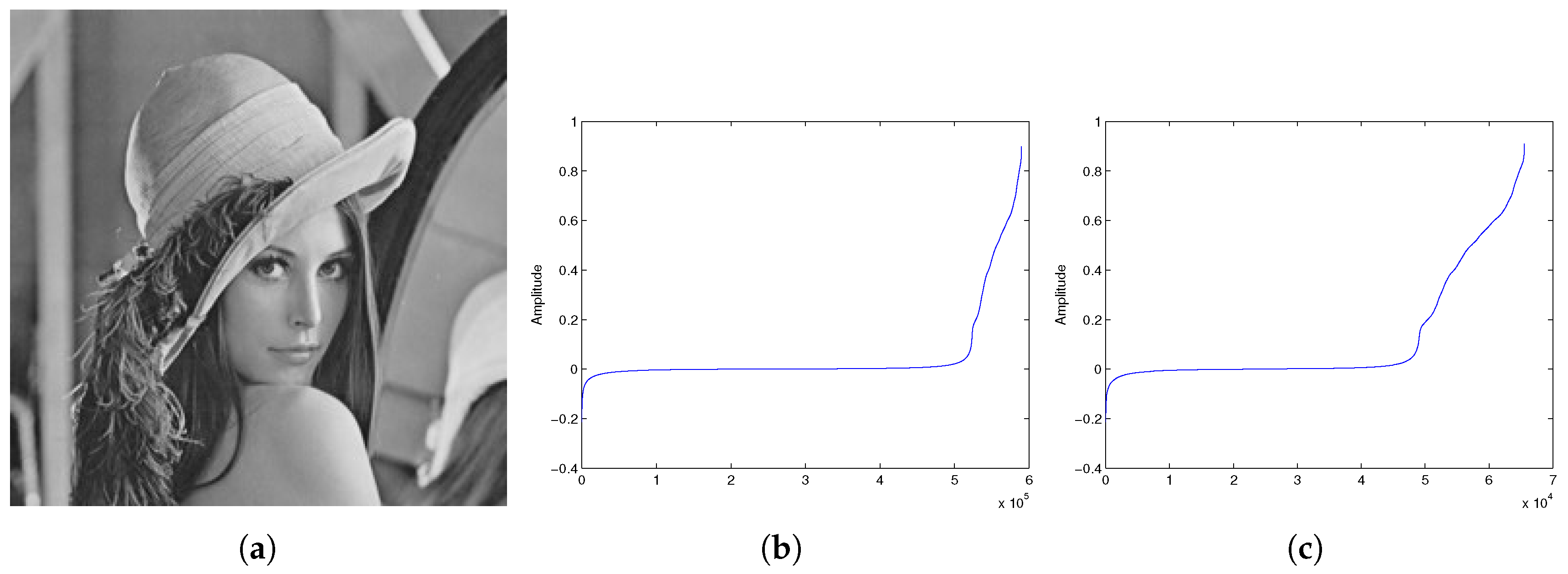
3. Transform Domains

3.1. Orthogonal Basis-Wavelet

The wavelet transform (WT) is a useful tool to provide a time-frequency representation of a signal. For a mother wavelet $\psi (t)$, the WT of the signal of interest (SOI) of $x(t)$ is given by [25]

$$\begin{array}{c}\hfill \begin{array}{c}\hfill {\mathrm{CWT}}_x(a,b)=\frac{1}{a^{-1/2}}{\int }_{-\infty }^{\infty }x(t){\psi }^{*}(\frac{t-b}{a})dt,\end{array}\end{array}$$

(5)

where * is the complex conjugate, and a and b respectively represent the scaling and translation factors. From Equation $(5)$, the scale parameter a compresses the wavelet when it is small. By doing so, the rapidly changing details of the signal are revealed. When it is large, it stretches the wavelet and, therefore, the coarse features of the signal are revealed.

The inverse WT is expressed

$$\begin{array}{c}\hfill \begin{array}{c}\hfill x(t)=\frac{C_{\psi }^{-1}}{a^{-1/2}}{\int }_{-\infty }^{\infty }{\int }_{-\infty }^{\infty }{\mathrm{CWT}}_x(a,b)\tilde{\psi }(\frac{t-b}{a})db\frac{da}{a^2},\end{array}\end{array}$$

(6)

where $\tilde{\psi }(t)$ denotes the dual function of $\psi (t)$ and $C_{\psi }^{-1}$ represents the admissible constant.

In a vector representation, matrix ${\mathcal{W}}_{WT}$ is utilized to represent the wavelet decomposition and ${\mathcal{W}}_{WT}^{\mathrm{T}}$ denotes the wavelet reconstruction. Using these notations, the image in wavelet domain is

$$\begin{array}{c}\hfill \begin{array}{c}\hfill {\mathbf{\alpha }}_{WT}={\mathcal{W}}_{WT}\mathbf{x},\end{array}\end{array}$$

(7)

and correspondingly the image is reconstructed by

$$\begin{array}{c}\hfill \begin{array}{c}\hfill \mathbf{x}={\mathcal{W}}_{WT}^{\mathrm{T}}{\mathbf{\alpha }}_{WT}.\end{array}\end{array}$$

(8)

It is well known that the wavelet coefficient ${\mathbf{\alpha }}_{WT}$ of the image contains many negligible components, which means ${\mathbf{\alpha }}_{WT}$ is sparse—for more information, see [25,26].

3.2. Nonorthogonal Basis-Framelet

A wavelet frame system provides better smoothness, short support and symmetrical property than the orthogonal wavelet basis by sacrificing orthonormality and linear independence [27].

With a scaling function $\varphi$ and wavelet functions $\{{\phi }_1,\dots ,{\phi }_r\}$, the so-called refinable equations are

$$\begin{array}{c}\hfill \begin{array}{c}\varphi (t)=\sqrt{2}\sum _k{h}_0(k)\varphi (2t-k),\hfill \\ {\phi }_l(t)=\sqrt{2}\sum _k{h}_l(k)\varphi (2t-k),l=1,2,\dots ,r,\hfill \end{array}\end{array}$$

(9)

where $\varphi (t)$, $\phi (t)$, and $h(t)$ are user defined functions, and, in this work, they are chosen the same as in [27]—for example, $h_0=\frac{1}{4}[1,2,1]$, $h_1=\frac{\sqrt{2}}{4}[1,0,-1]$, and $h_2=\frac{1}{4}[-1,2,-1]$, and $\varphi (t)$, $\phi (t)$ are the piecewise linear refinable spline and corresponding framelets.

Under these notations, the frame coefficients of a signal $x(t)$ can be calculated as

$$\begin{array}{c}\hfill \begin{array}{c}{c}_k=\int x(t){\varphi }_k(t)dt,\hfill \\ d_{k,j,l}=\int x(t){\phi }_{k,j,l}(t)dt,\hfill \end{array}\end{array}$$

(10)

where $c_k$ and $d_{k,j,l}$ are the frame coefficients, and ${\varphi }_k(t)=\varphi (t-k)$, ${\phi }_{k,j,l}(t)={\phi }_l(2^{j}t-k)$.

With the frame coefficients, the signal is synthesized as

$$\begin{array}{c}\hfill \begin{array}{c}\hfill x(t)=\sum _{k=-\infty }^{\infty }{c}_k{\varphi }_k(t)+\sum _{l=1}^r\sum _{j=0}^{\infty }\sum _{k=-\infty }^{\infty }{d}_{k,j,l}{\phi }_{k,j,l}.\end{array}\end{array}$$

(11)

Similarly, ${\mathcal{W}}_{FT}$ is utilized to represent the tensor product framelet decomposition and ${\mathcal{W}}_{FT}^{\mathrm{T}}$ denotes the framelet reconstruction, and, therefore, in the matrix notation, the frame coefficient and reconstructed image are respectively calculated by

$$\begin{array}{c}\hfill \begin{array}{c}\hfill {\mathbf{\alpha }}_{FT}={\mathcal{W}}_{FT}\mathbf{x},\mathbf{x}={\mathcal{W}}_{FT}^{\mathrm{T}}{\mathbf{\alpha }}_{FT}.\end{array}\end{array}$$

(12)

Two representative bases are briefly introduced—for more details, the diligent readers are referred to [25,27], especially [25] for the wavelet transform and [27] for the framelet transform. It is of interest to note that there are other transform domains that can be exploited for images—for example, second-generation wavelet [28] and synchrosqueezed wavelet transforms (SST) [29], to name a few. However, the further studies of different domains are beyond scope of this work. To more clearly observe the difference of two bases, the following experiment is conducted, where the coefficients of the framelet and wavelet decompositions are provided in Figure 1. It is clearly seen that framelet decomposition produces more sparse representation of the image than the wavelet one. Therefore, it is expected that framelet based approach will outperform the wavelet based approach.

4. Problem Formulation and Algorithm Development

With the sparse representation in the transform domain, the degraded image in Equation $(3)$ is reexpressed more explicitly as

$$\begin{array}{c}\hfill \begin{array}{c}\hfill \tilde{\mathbf{y}}=\mathbf{H}({\mathcal{W}}_{WT,FT}^{\mathrm{T}}{\mathbf{\alpha }}_{WT,FT})+\tilde{\mathbf{n}},\end{array}\end{array}$$

(13)

where ${\mathcal{W}}_{WT,FT}$ respectively indicates the wavelet and framelet transform operator and ${\mathbf{\alpha }}_{WT,FT}$ is the transform coefficient vector in the corresponding domain. To utilize the sparse property of the ${\mathbf{\alpha }}_{WT,FT}$, $\mathbf{H}$, and $\mathbf{n}$, the following optimization problem is developed to jointly conduct image reconstruction and missing pattern estimation in the case of the salt-and-pepper noise. That is,

$$\begin{array}{c}\hfill \begin{array}{c}\mathrm{minimize}\parallel {\mathbf{\alpha }}_{WT,FT}{\parallel }_1+{\lambda }_1{\parallel \mathbf{H}\parallel }_1+{\lambda }_2{\parallel \tilde{\mathbf{n}}\parallel }_1\hfill \\ \mathrm{subject}\mathrm{to}\parallel \tilde{\mathbf{y}}-\mathbf{H}({\mathcal{W}}_{WT,FT}^{\mathrm{T}}{\mathbf{\alpha }}_{WT,FT})-\tilde{\mathbf{n}}{\parallel }_2^2<ϵ,\hfill \end{array}\end{array}$$

(14)

with variables ${\mathbf{\alpha }}_{WT,FT}$, $\mathbf{H}$ and $\tilde{\mathbf{n}}$. To efficiently solve the optimization problem in Equation $(14)$, a two-step process is utilized. Let us first suppose that $\mathbf{H}$ is known; the sub-problem is a convex optimization problem with variables ${\mathbf{\alpha }}_{WT,FT}$ and $\tilde{\mathbf{n}}$. Second, with the estimated values of ${\mathbf{\alpha }}_{WT,FT}$ and $\tilde{\mathbf{n}}$, the sub-problem is another convex optimization with variable $\mathbf{H}$. In Equation $(14)$, the parameter of $ϵ$ is usually chosen empirically, but some approaches such as factor model can be utilized to obtain the optimal value [30]. To summarize, the two-step procedure is as follows:

Initialize missing pattern vector.

• $\mathbf{Step}\mathbf{1}$: Solve Equation $(14)$ with the initialized/estimated missing pattern to obtain estimations of ${\mathbf{\alpha }}_{WT,FT}$ and $\tilde{\mathbf{n}}$ as

  $$\begin{array}{c}\hfill \begin{array}{c}\mathrm{minimize}\parallel {\mathbf{\alpha }}_{WT,FT}{\parallel }_1+{\lambda }_2{\parallel \tilde{\mathbf{n}}\parallel }_1\hfill \\ \mathrm{subject}\mathrm{to}\parallel \tilde{\mathbf{y}}-\widehat{\mathbf{H}}({\mathcal{W}}_{WT,FT}^{\mathrm{T}}{\mathbf{\alpha }}_{WT,FT})-\tilde{\mathbf{n}}{\parallel }_2<ϵ,\hfill \end{array}\end{array}$$

  (15)

  where $\widehat{\mathbf{H}}$ is the initialized/estimated value of the missing pattern.
• $\mathbf{Step}\mathbf{2}$: With the estimations from Step 1, solving Equation $(14)$ yields missing pattern estimation as

  $$\begin{array}{c}\hfill \begin{array}{c}{\mathrm{minimize}\parallel \mathbf{H}\parallel }_1\hfill \\ \mathrm{subject}\mathrm{to}\parallel \tilde{\mathbf{y}}-\mathbf{H}({\mathcal{W}}_{WT,FT}^{\mathrm{T}}{\widehat{\mathbf{\alpha }}}_{WT,FT})-\widehat{\tilde{\mathbf{n}}}{\parallel }_2<ϵ,\hfill \end{array}\end{array}$$

  (16)

  where ${\widehat{\mathbf{\alpha }}}_{WT,FT}$ and $\widehat{\tilde{\mathbf{n}}}$ denote the estimated values of ${\mathbf{\alpha }}_{WT,FT}$ and $\tilde{\mathbf{n}}$, respectively.
• Iterate Steps 1 and 2 until a stopping rule is met.

It is seen that at each step, it solves an ${\ell }_1$-norm constrained optimization problem, and considering the large size of the image, the following two algorithms of ADMM and APG are tailored to solve the optimization problems.

4.1. Alternating Direction Method of Multipliers (ADMM)

To efficiently solve the optimization problems of Equations $(15)$ and $(16)$, in this paper, the ADMM approach  [31] is utilized in which the dual ascent and method of multipliers are utilized recursively.

In light of ADMM approach, consider the Step 1 in Equation $(15)$ first, and since the optimizations of $\mathbf{n}$ and $\mathbf{\alpha }$ are separable, the estimation of $\mathbf{n}$ is rewritten as

$$\begin{array}{c}\hfill \begin{array}{c}\mathrm{minimize}\parallel \mathbf{y}-\widehat{\mathbf{H}}{\mathbf{n}\parallel }_2^2+\lambda {\parallel \mathbf{n}\parallel }_1\hfill \end{array}\end{array}$$

(17)

with variable $\mathbf{n}$, where the subscripts are omitted to simplify the notation expression and $\lambda$ is the regularization parameter. For this problem, the ADMM steps for estimating the $\mathbf{n}$ at lth iteration are given by

$$\begin{array}{c}\hfill \begin{array}{c}{\mathbf{n}}^{l+1}={\mathrm{minimize}}_{\mathbf{n}}\left(\parallel \mathbf{y}-\widehat{\mathbf{H}}{\mathbf{n}\parallel }_2^2+(\rho /2){\parallel \mathbf{n}-{\mathbf{z}}^l+{\mathbf{s}}^l\parallel }_2^2\right),\hfill \\ {\mathbf{z}}^{l+1}={\mathrm{minimize}}_{\mathbf{z}}\left({\lambda \parallel \mathbf{z}\parallel }_1+(\rho /2){\parallel {\mathbf{n}}^{l+1}-\mathbf{z}+{\mathbf{s}}^l\parallel }_2^2\right),\hfill \\ {\mathbf{s}}^{l+1}={\mathbf{s}}^l+{\mathbf{r}}^{l+1}-{\mathbf{z}}^{l+1}.\hfill \end{array}\end{array}$$

(18)

In the $\mathbf{n}$-step of Equation $(18)$, setting the derivative of the cost function with respect to $\mathbf{n}$ to zero yields

$$\begin{array}{c}\hfill \begin{array}{c}\hfill -2{\widehat{\mathbf{H}}}^{\mathrm{H}}\mathbf{y}+2{\widehat{\mathbf{H}}}^{\mathrm{H}}\widehat{\mathbf{H}}\mathbf{n}+\rho (\mathbf{n}-{\mathbf{z}}^l+{\mathbf{s}}^l)=0.\end{array}\end{array}$$

(19)

Rearranging the terms in Equation $(19)$ produces

$$\begin{array}{c}\hfill \begin{array}{c}\hfill (\rho \mathbf{I}+2{\widehat{\mathbf{H}}}^{\mathrm{H}}\widehat{\mathbf{H}})\mathbf{n}=\rho ({\mathbf{z}}^l-{\mathbf{s}}^l)+2{\widehat{\mathbf{H}}}^{\mathrm{H}}\mathbf{y}.\end{array}\end{array}$$

(20)

By the use of Equation $(20)$, the estimate of $\mathbf{n}$ in a closed-form expression is

$$\begin{array}{c}\hfill \begin{array}{c}\hfill \mathbf{n}={(\rho \mathbf{I}+2{\widehat{\mathbf{H}}}^{\mathrm{H}}\widehat{\mathbf{H}})}^{-1}(\rho ({\mathbf{z}}^l-{\mathbf{s}}^l)+2{\widehat{\mathbf{H}}}^{\mathrm{H}}\mathbf{y}).\end{array}\end{array}$$

(21)

In the $\mathbf{z}$-step of Equation $(18)$, according to subdifferential calculus, the estimate of $\mathbf{z}$ is obtained by componentwise soft thresholding as

$$\begin{array}{c}\hfill \begin{array}{c}\hfill {\mathbf{z}}^{l+1}={\mathbf{T}}_{\lambda /\rho }\left({\mathbf{n}}^{l+1}+{\mathbf{s}}^l\right),\end{array}\end{array}$$

(22)

where the soft thresholding operator $\mathbf{T}$ is given by

$$\begin{array}{cc}\hfill {\mathbf{T}}_{\lambda /\rho }(a)& =\left\{\begin{array}{cc}a-\lambda /\rho ,& a>\lambda /\rho ,\\ 0,& \left|a\right|<\lambda /\rho ,\\ a+\lambda /\rho ,& a<-\lambda /\rho .\end{array}\right.\hfill \end{array}$$

(23)

It is documented that soft thresholding is the proximity operator of the ${\ell }_1$ norm—see [31].

To estimate $\mathbf{\alpha }$, without ambiguity, the subscript of $\mathcal{W}$ is dropped, and the optimization problem now is

$$\begin{array}{c}\hfill \begin{array}{c}\mathrm{minimize}\parallel \mathbf{y}-\widehat{\mathbf{H}}\mathcal{W}\mathbf{\alpha }-\widehat{\mathbf{n}}{\parallel }_2^2+\lambda {\parallel \mathbf{\alpha }\parallel }_1.\hfill \end{array}\end{array}$$

(24)

Similarly, the ADMM steps of $\mathbf{\alpha }$ at lth iteration are

$$\begin{array}{c}\hfill \begin{array}{c}{\mathbf{\alpha }}^{l+1}={\mathrm{minimize}}_{\mathbf{\alpha }}\left(\parallel \mathbf{y}-\widehat{\mathbf{H}}\mathcal{W}\mathbf{\alpha }-\widehat{\mathbf{n}}{\parallel }_2^2+(\rho /2){\parallel \mathbf{\alpha }-{\mathbf{g}}^l+{\mathbf{u}}^l\parallel }_2^2\right)\hfill \\ {\mathbf{g}}^{l+1}={\mathrm{minimize}}_{\mathbf{g}}\left({\lambda \parallel \mathbf{g}\parallel }_1+(\rho /2){\parallel {\mathbf{\alpha }}^{l+1}-\mathbf{g}+{\mathbf{u}}^l\parallel }_2^2\right)\hfill \\ {\mathbf{u}}^{l+1}={\mathbf{u}}^l+{\mathbf{\alpha }}^{l+1}-{\mathbf{g}}^{l+1}.\hfill \end{array}\end{array}$$

(25)

By the steps developed in Equations (19)–(23), the estimates for $\mathbf{\alpha }$ and $\mathbf{g}$ can be respectively obtained by

$$\begin{array}{c}\hfill \begin{array}{c}\hfill \mathbf{\alpha }={(\rho \mathbf{I}+2{\mathcal{W}}^{\mathrm{H}}{\widehat{\mathbf{H}}}^{\mathrm{H}}\widehat{\mathbf{H}}\mathcal{W})}^{-1}(\rho ({\mathbf{g}}^l-{\mathbf{u}}^l)+2{\mathcal{W}}^{\mathrm{H}}(\mathbf{y}-\widehat{\mathbf{n}})),\end{array}\end{array}$$

(26)

$$\begin{array}{c}\hfill \begin{array}{c}\hfill {\mathbf{g}}^{l+1}={\mathbf{T}}_{\lambda /\rho }\left({\mathbf{\alpha }}^{l+1}+{\mathbf{u}}^l\right).\end{array}\end{array}$$

(27)

Now, we turn our attention into solving the Step 2 in Equation $(16)$, and its ADMM steps are

$$\begin{array}{c}\hfill \begin{array}{c}{\mathbf{H}}^{l+1}={\mathrm{minimize}}_{\mathbf{H}}\left(\parallel \mathbf{y}-\mathbf{H}(\mathcal{W}\widehat{\mathbf{\alpha }}+\widehat{\mathbf{n}}){\parallel }_2^2+(\rho /2){\parallel \mathbf{H}-{\mathbf{Z}}^l+{\mathbf{U}}^l\parallel }_{\mathrm{F}}^2\right)\hfill \\ {\mathbf{Z}}^{l+1}={\mathrm{minimize}}_{\mathbf{Z}}\left({\lambda \parallel \mathbf{Z}\parallel }_1+(\rho /2){\parallel {\mathbf{H}}^{l+1}-\mathbf{Z}+{\mathbf{U}}^l\parallel }_{\mathrm{F}}^2\right)\hfill \\ {\mathbf{U}}^{l+1}={\mathbf{U}}^l+{\mathbf{H}}^{l+1}-{\mathbf{Z}}^{l+1}.\hfill \end{array}\end{array}$$

(28)

Similarly, the estimates of $\mathbf{H}$ and $\mathbf{Z}$ are respectively calculated by

$$\begin{array}{c}\hfill \begin{array}{c}\hfill \mathbf{H}={(\rho \mathbf{I}+2{(\mathcal{W}\widehat{\mathbf{\alpha }}+\widehat{\mathbf{n}})}^{\mathrm{H}}(\mathcal{W}\widehat{\mathbf{\alpha }}+\widehat{\mathbf{n}}))}^{-1}(\rho ({\mathbf{Z}}^l-{\mathbf{U}}^l)\\ \hfill +2{(\mathcal{W}\widehat{\mathbf{\alpha }}+\widehat{\mathbf{n}})}^{\mathrm{H}}\mathbf{y}),\end{array}\end{array}$$

(29)

$$\begin{array}{c}\hfill \begin{array}{c}\hfill \mathbf{Z}={\mathbf{T}}_{\lambda /\rho }\left({\mathbf{H}}^{l+1}+{\mathbf{U}}^l\right).\end{array}\end{array}$$

(30)

In accordance with Equation $(29)$, as one sees, the terms of $\mathcal{W}$ and $\mathbf{y}$ are known in this step and, therefore, the ${(\rho \mathbf{I}+{(\mathcal{W}\widehat{\mathbf{\alpha }}+\widehat{\mathbf{n}})}^{\mathrm{H}}(\mathcal{W}\widehat{\mathbf{\alpha }}+\widehat{\mathbf{n}}))}^{-1}$ and ${(\mathcal{W}\widehat{\mathbf{\alpha }}+\widehat{\mathbf{n}})}^{\mathrm{H}}\mathbf{y}$ can be computed in advance to save the computational complexity. With the ADMM steps developed, the algorithm to solve Equation $(14)$ is summarized in Algorithm  1.

Algorithm 1 Alternating Direction Method of Multipliers (ADMM) based approach.

Objective function: ${\lambda }_1\parallel {\mathbf{\alpha }}_{WT,FT}{\parallel }_1+{\lambda }_2{\parallel \mathbf{H}\parallel }_1+{\lambda }_3{\parallel \mathbf{n}\parallel }_1+{\parallel \tilde{\mathbf{y}}-\mathbf{H}({\mathcal{W}}_{WT,FT}^{\mathrm{T}}{\mathbf{\alpha }}_{WT,FT}+\mathbf{n})\parallel }_2^2$

Outputs: Estimates of $\mathbf{n}$, $\mathbf{\alpha }$ and $\mathbf{H}$

Initialization: $l=1$Repeat

$l=l+1$

Step 1: Produce the estimate of $\mathbf{n}$ by Equations $(18)$–$(23)$

Step 2: Produce the estimate of $\mathbf{\alpha }$ by Equations $(25)$–$(27)$

Step 2: Produce the estimate of $\mathbf{H}$ by Equations $(29)$ and $(30)$

Step 3: Update the residual $\tilde{\mathbf{y}}=\tilde{\mathbf{y}}-\mathbf{H}({\mathcal{W}}_{WT,FT}^{\mathrm{T}}{\mathbf{\alpha }}_{WT,FT}+\mathbf{n})$

Until$l>T$ {maximum iteration} or $\mathrm{norm}(\tilde{\mathbf{y}})<\delta$ {predefined threshold}.

4.2. Accelerated Proximal Gradient (APG)

In addition to ADMM, the accelerated proximal gradient (APG) approach has been widely utilized to solve ${\ell }_1$-norm regularization problem because of its fast convergence and excellent performance  [32,33]. It is developed for the following unconstrained optimization problem:

$$\begin{array}{c}\hfill \begin{array}{c}\hfill \mathrm{minimize}F(x)+G(x),\end{array}\end{array}$$

(31)

with variable x. In the APG algorithm, when the second function is ${\ell }_1$-norm, namely $G(x)={\lambda \parallel x\parallel }_1$, the update of x is obtained by the soft-thresholding operator, given by

$$\begin{array}{c}\hfill \begin{array}{c}\hfill x_{k+1}={\mathbf{T}}_{\lambda /L}({\beta }_l-\frac{1}{L}\nabla F({\beta }_l)).\end{array}\end{array}$$

(32)

For our problem, let $F(\mathbf{\alpha },\mathbf{n},\mathbf{H})=\parallel \tilde{\mathbf{y}}-\mathbf{H}({\mathcal{W}}^{\mathrm{T}}\mathbf{\alpha }+\mathbf{n}){\parallel }_2^2$ and $G(\mathbf{\alpha })={\lambda }_1{\parallel \mathbf{\alpha }\parallel }_1,G(\mathbf{n})={\lambda }_2{\parallel \mathbf{n}\parallel }_1,G(\mathbf{H})={\lambda }_3{\parallel \mathbf{H}\parallel }_1$; then, calculate the gradients of $F(\mathbf{\alpha },\mathbf{n},\mathbf{H})$ with respect to $\mathbf{\alpha }$, $\mathbf{n}$, $\mathbf{H}$, respectively. With simple calculations, the gradients are of the form

$$\begin{array}{c}\hfill \begin{array}{c}{\nabla }_{\mathbf{n}}F(\mathbf{\alpha },\mathbf{n},\mathbf{H})=-2{\mathbf{H}}^{\mathrm{H}}(\mathbf{y}-\mathbf{H}\mathcal{W}\mathbf{\alpha }-\mathbf{H}\mathbf{n}),\hfill \\ {\nabla }_{\mathbf{\alpha }}F(\mathbf{\alpha },\mathbf{n},\mathbf{H})=-2{\mathcal{W}}^{\mathrm{H}}{\mathbf{H}}^{\mathrm{H}}(\mathbf{y}-\mathbf{H}\mathcal{W}\mathbf{\alpha }-\mathbf{H}\mathbf{n}),\hfill \\ {\nabla }_{\mathbf{H}}F(\mathbf{\alpha },\mathbf{n},\mathbf{H})=-2{({\mathcal{W}}^{\mathrm{T}}\mathbf{\alpha }+\mathbf{n})}^{\mathrm{H}}(\mathbf{y}-\mathbf{H}\mathcal{W}\mathbf{\alpha }-\mathbf{H}\mathbf{n}).\hfill \end{array}\end{array}$$

(33)

With those gradients, the APG based approach to solve Equation $(14)$ is now summarized in Algorithm 2.

Algorithm 2 Accelerated Proximal Gradient (APG) based approach.

Objective function: ${\lambda }_1\parallel {\mathbf{\alpha }}_{WT,FT}{\parallel }_1+{\lambda }_2{\parallel \mathbf{H}\parallel }_1+{\lambda }_3{\parallel \mathbf{n}\parallel }_1+{\parallel \tilde{\mathbf{y}}-\mathbf{H}({\mathcal{W}}_{WT,FT}^{\mathrm{T}}{\mathbf{\alpha }}_{WT,FT}+\mathbf{n})\parallel }_2^2$

Outputs: Estimates of $\mathbf{n}$, $\mathbf{\alpha }$ and $\mathbf{H}$

Initialization: $l=0$, ${\mathbf{n}}_0={\mathbf{n}}_{-1}$, ${\mathbf{\alpha }}_0={\mathbf{\alpha }}_{-1}$, ${\mathbf{H}}_0={\mathbf{H}}_{-1}$$t_0=1,t_{-1}=0$

Repeat

${\beta }_l^{\mathbf{n}}={\mathbf{n}}_l+\frac{t_{l-1}}{t_l}({\mathbf{n}}_l-{\mathbf{n}}_{l-1})$

${\beta }_l^{\mathbf{\alpha }}={\mathbf{\alpha }}_l+\frac{t_{l-1}}{t_l}({\mathbf{\alpha }}_l-{\mathbf{\alpha }}_{l-1})$

${\beta }_l^{\mathbf{H}}={\mathbf{H}}_l+\frac{t_{l-1}}{t_l}({\mathbf{H}}_l-{\mathbf{H}}_{l-1})$

${\mathbf{n}}_{l+1}={\mathbf{T}}_{{\lambda }_1/L}({\beta }_l^{\mathbf{n}}-{\nabla }_{\mathbf{n}}F({\beta }_l^{\mathbf{n}},{\beta }_l^{\mathbf{\alpha }},{\beta }_l^{\mathbf{H}})/L)$

${\mathbf{\alpha }}_{l+1}={\mathbf{T}}_{{\lambda }_2/L}({\beta }_l^{\mathbf{\alpha }}-{\nabla }_{\mathbf{\alpha }}F({\beta }_l^{\mathbf{n}},{\beta }_l^{\mathbf{\alpha }},{\beta }_l^{\mathbf{H}})/L)$

${\mathbf{H}}_{l+1}={\mathbf{T}}_{{\lambda }_3/L}({\beta }_l^{\mathbf{H}}-{\nabla }_{\mathbf{H}}F({\beta }_l^{\mathbf{n}},{\beta }_l^{\mathbf{\alpha }},{\beta }_l^{\mathbf{H}})/L)$

$t_{l+1}=\frac{1+\sqrt{1+4t_l^2}}{2}$

$l=l+1$

Until$l>T$ {maximum iteration} or $\parallel {\mathcal{W}}^{\mathrm{T}}({\mathbf{\alpha }}_{l+1}-{\mathbf{\alpha }}_l){\parallel }_2<\delta$ {predefined threshold}.

5. Numerical Studies

The numerical studies are conducted in this section to show the performance of the proposed joint estimation method. For comparison purposes, the results from adaptive median filter and edge preserving regularization (AM-IEPR) [11], standard median (MED) filter [6], adaptive median filter (AMF) [7], beta process factor analysis (BPFA) [4], and fields of experts (FoE) [16] are also provided. In simulations, for ADMM, the parameters of $\lambda$, $\rho$ and T for the estimation of n are chosen as 0.25, 0.25 and 700, the parameters of $\lambda$, $\rho$ and T for the estimation of $\alpha$ are chosen as 0.75, 0.075 and 700, the parameters of $\lambda$, $\rho$ and T for the estimation of $\mathbf{H}$ are chosen as 7.5, 750 and 50, and the maximum iteration of $\mathbf{n}$, $\alpha$ and $\mathbf{H}$ are set to be 3. For APG, the parameters of $\lambda$, L and T for the estimation of n are chosen as 0.00045, 3 and 500, the parameters of $\lambda$, L and T for the estimation of $\alpha$ are chosen as 0.0003, 3 and 500, the parameters of $\lambda$, L and T for the estimation of $\mathbf{H}$ are chosen as 0.0002, 3 and 20, and the maximum iteration of $\mathbf{n}$, $\alpha$ and $\mathbf{H}$ are also set to be 3. The performance evaluations are quantitatively measured by means of the peak signal-to-noise ratio (PSNR), the mean absolute error (MAE) and the structural similarity index (SSIM), and they are of the form

$$\begin{array}{c}\hfill \begin{array}{c}\mathrm{PSNR}=10{\log }_{10}\frac{{255}^2}{\frac{1}{\mathrm{MN}}{\sum }_{i,j}{(r_{i,j}-x_{i,j})}^2},\hfill \\ \mathrm{MAE}=\frac{1}{\mathrm{MN}}\sum _{i,j}\left|(r_{i,j}-x_{i,j})\right|,\hfill \\ \mathrm{SSIM}(x,y)=\frac{(2{\mu }_x{\mu }_y+c_1)(2{\sigma }_{xy}+c_2)}{({\mu }_x^2+{\mu }_y^2+c_1)({\sigma }_x^2+{\sigma }_y^2+c_2)},\hfill \end{array}\end{array}$$

(34)

where $r_{i,j}$ and $x_{i,j}$ denote the pixel values of the reconstructed image and the original image, respectively, ${\mu }_x$ and ${\mu }_y$ respectively denote the average of x and y, ${\sigma }_x^2$ and ${\sigma }_y^2$ are the variances of x and y, ${\sigma }_{xy}$ is the covariance of x and y, $c_1={(k_{1}P)}^2$, $c_2={(k_{2}P)}^2$ are two variables to stabilize the division with weak denominator, P is the dynamic range of the pixel-values, and $k_1=0.01$ and $k_2=0.03$ are chosen by default.

5.1. Salt-and-Pepper Noise Only

In this section, the latent image corrupted by the salt-and-pepper only is studied first. Figure 2 depicts the restoration results of different algorithms under $70\%$ noise level. Generally speaking, the APG based solver provides better recovery performance than ADMM based solver, demonstrated in Figure 2c–f. Moreover, the framelt domain based recovery algorithms outperform the wavelet domain based algorithm because the nonorthogonality in the framelet improves the sparse representations. Therefore, the combination of framelet and APG, denoted by framelt+APG, outperforms all the other algorithms. Specifically, the $\mathit{lena}$ image reconstructed by framelt+APG shows the clean image with no noise residual, seen in Figure 2c. On the other hand, the best performance provided by the competing approaches is the AM-IEPR, but it still shows unclear effect, shown in Figure 2g. To observe the performance of the different algorithms in terms of the objective criterion, the results of PSNR, MAE and SSIM are provided in Figure 3, using 100 randomly selected images from SIPI Image Database. Inspecting Figure 3a shows that the framelt+APG produces the best PSNR index among all the methods, thereby yielding the best recovery performance, which is consistent with the conclusion in Figure 2. From the SSIM, it is seen that the value of the framelt+APG is very close to one, whereas the other algorithms drop significantly as the noise level increases.

5.2. Data Missing Only

In this section, the perforce of different algorithms is provided in the case of the data missing only. The original image and degraded image with 70% random missing are presented in Figure 4a,b, and the reconstructed images by proposed methods and other approaches are provided in Figure 4c–h. In this case, the framelet+APG approach is able to recover the original clean image in great details and hence produces the best PSNR of 29.1 dB. The second best PSNR is provided by the FoE approach, but burry effect is still present. In Figure 5, using 100 randomly selected images from SIPI Image Database, the indexes of PSNR, MAE and SSIM are provided in which the framelet+APG approach produces the best and consistent PSNR across the range of low and high missing levels. Especially, when the missing level is low, say 10%, the PSNR is more than 40 dB that is a 2 dB gain greater than the second best one, and when the missing level is high, say 70%, the PSNR obtained is still close to 35 dB. In addition to that, the value of the SSIM obtained by the framelet+APG is close to one even when the missing level is high as 70%. In summary, the recovery performance obtained by framelet+APG is satisfactory in terms of both visual and objective standards.

Figure 6 shows the restoration results of different algorithms under a specific data missing pattern. A text message imbedded in the clean image is given in Figure 6a. The reconstructed images are provided in Figure 6b–f. However, all the methods are able to recover the original image, but the image obtained by the framelet+APG is visually superior to other schemes. Judging from the close-up portion of the Figure 6, compared to the other images obtained, the great details of the image obtained by the framelet+APG approach are preserved, demonstrated in Figure 7. The recovered text images in Figure 8 show again that the framelet+APG algorithm produces best result, whereas the text recovered by wavelet+ADMM shows faded effect.

In practice, the illegal action of covering licence plate is somehow a common means to avoid penalties. To save manpower, the reconstruction of the original plate from the degraded one is desired, and the proposed methods are applied in attempt to that end. In order to simulate the illegal action, one number is completely missed in the original plate, shown in Figure 9b. In this data missing problem, the proposed approaches are applied to reconstruct the original plate and the results are provided in Figure 9c–f. It is observed that the APG based approaches are able to recover the original number, whereas there are still some missing parts in the image obtained by the ADMM based approaches. The experiment in this case is somehow ideal in the way that, if the intention is to avoid penalty, the entire plate will be covered. If that is the case, we suspect that the technology would not be of much use except for the local enforcements. Nonetheless, the proposed methods still will be useful in recovering the partially covered plates.

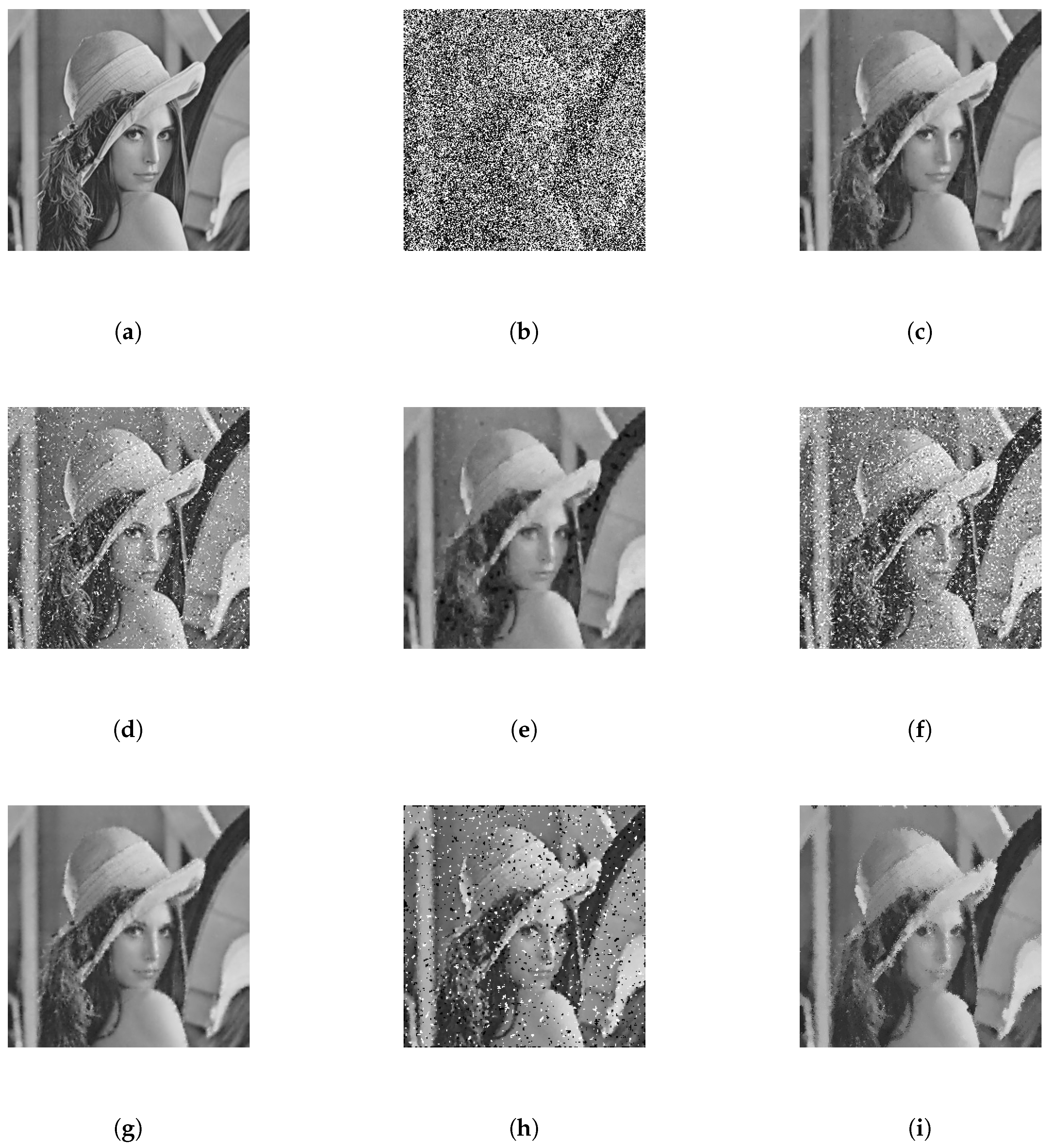
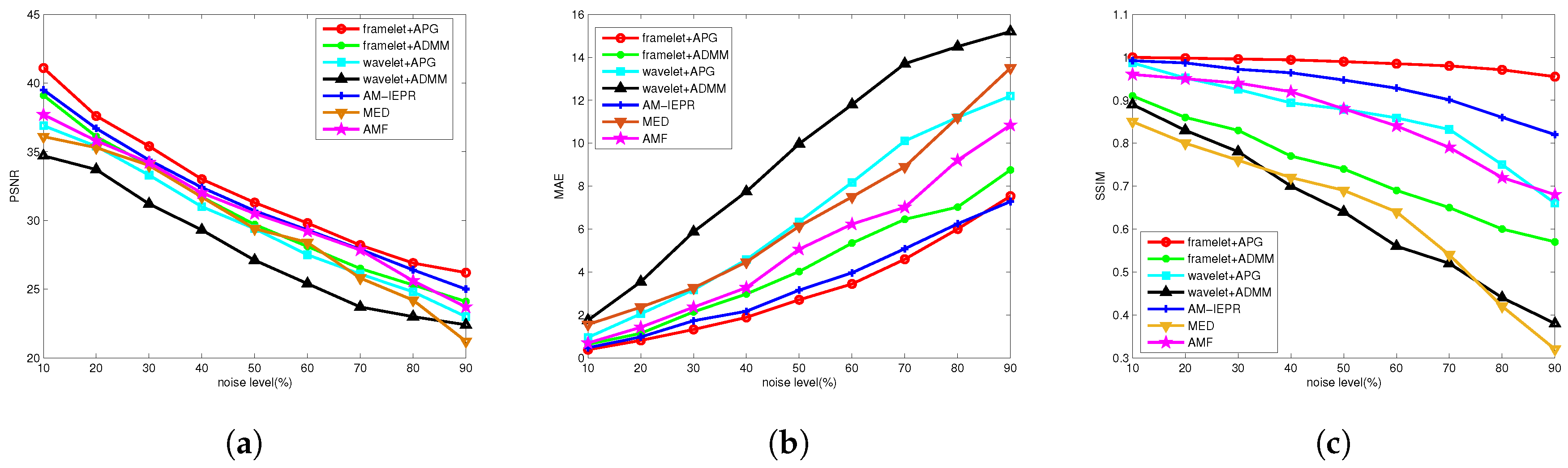
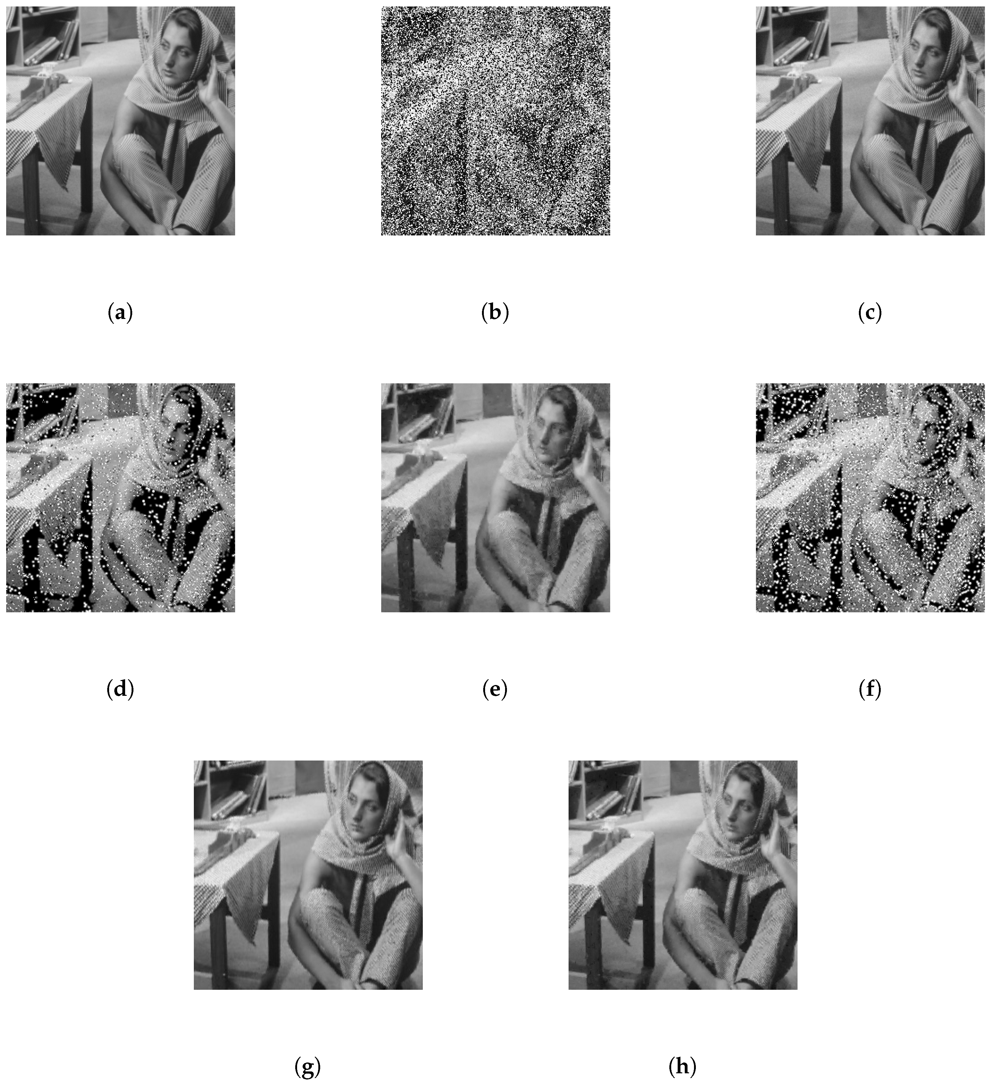
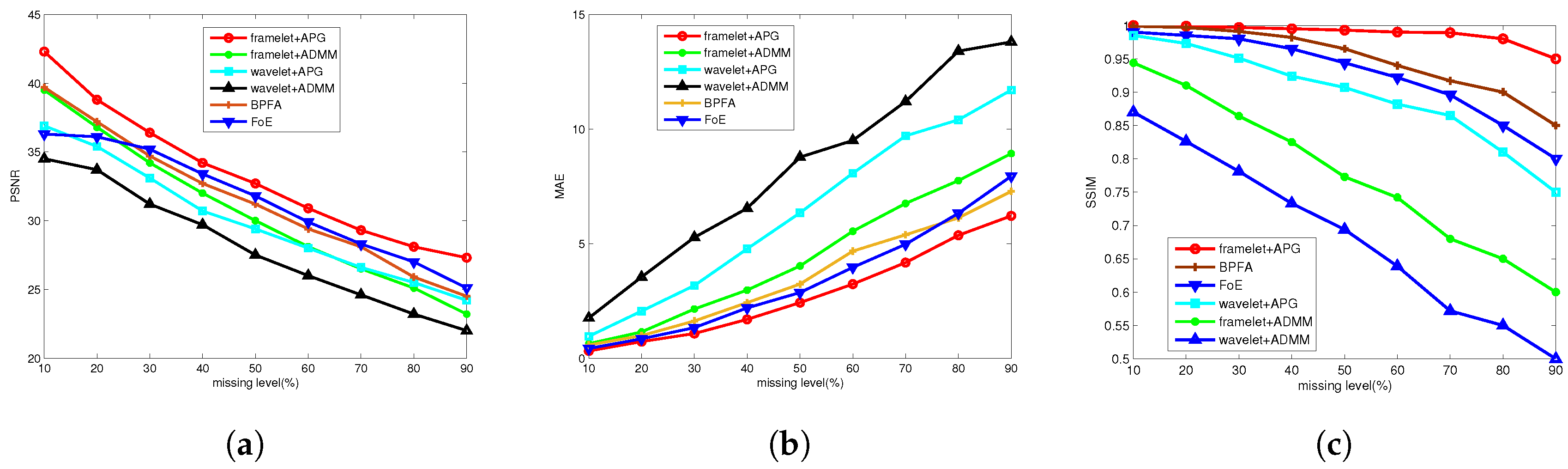
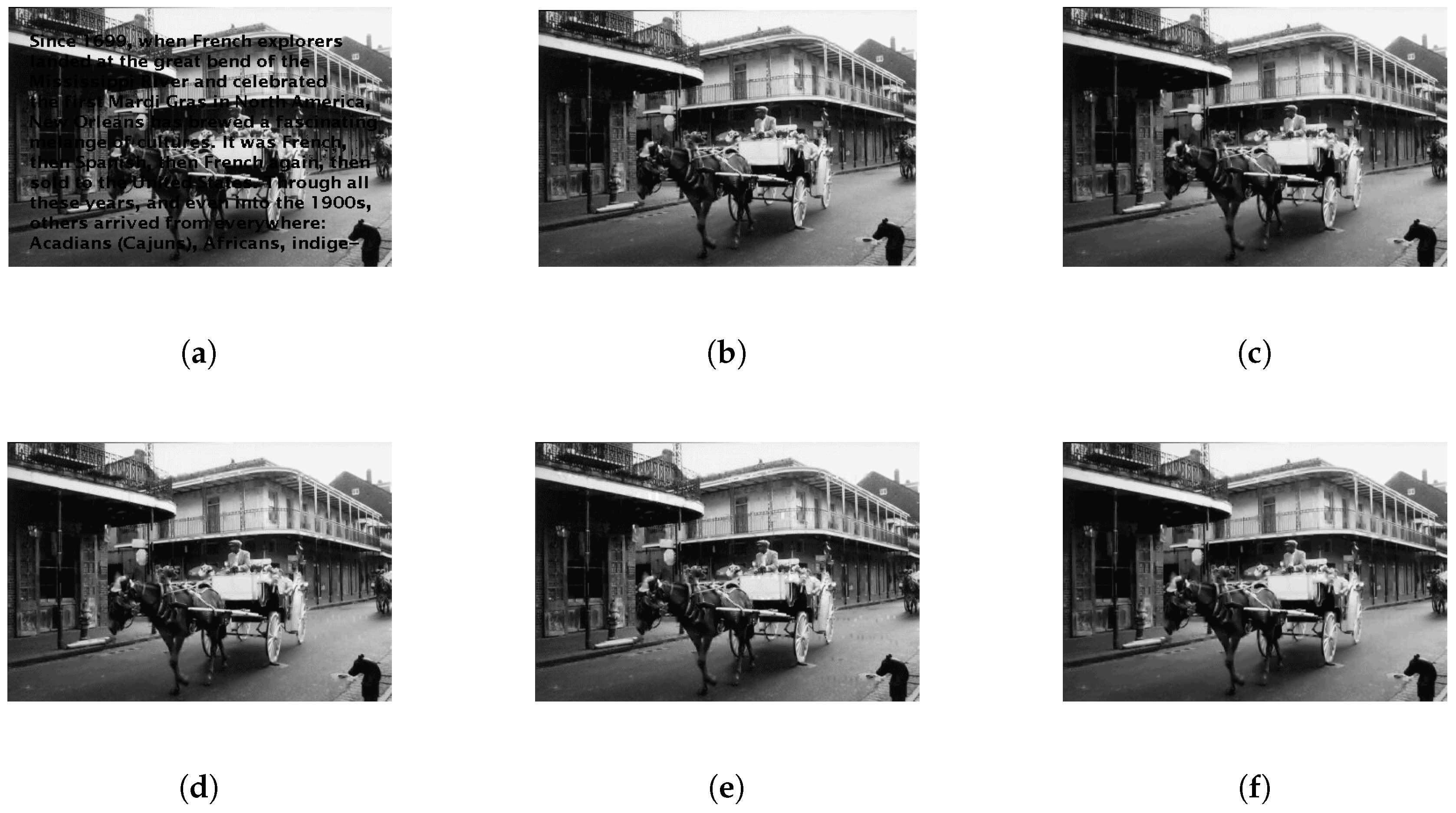
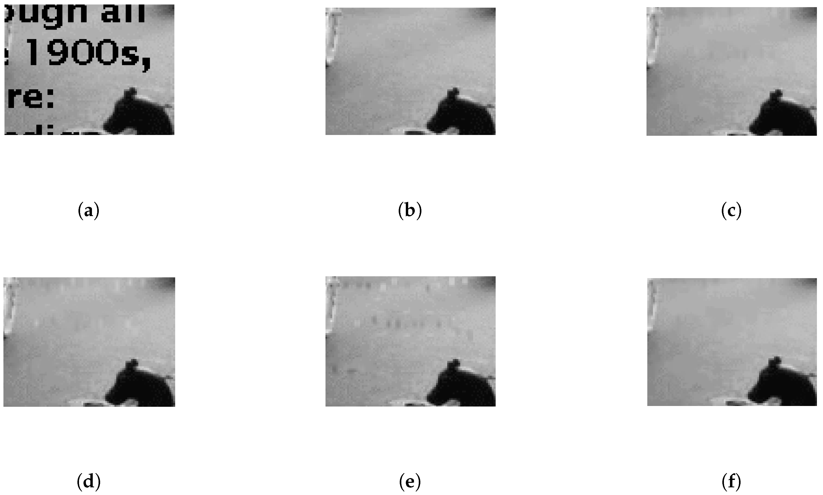
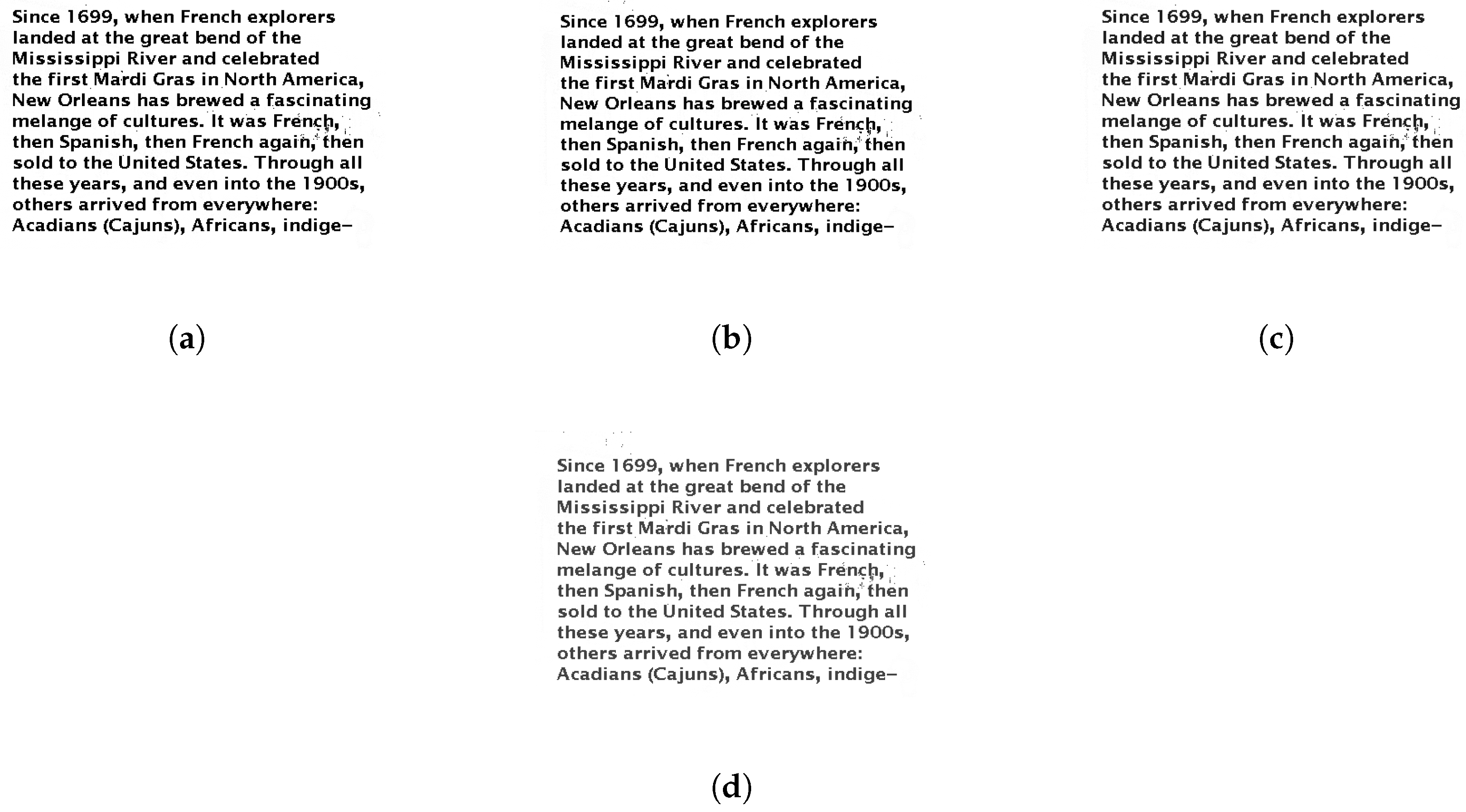
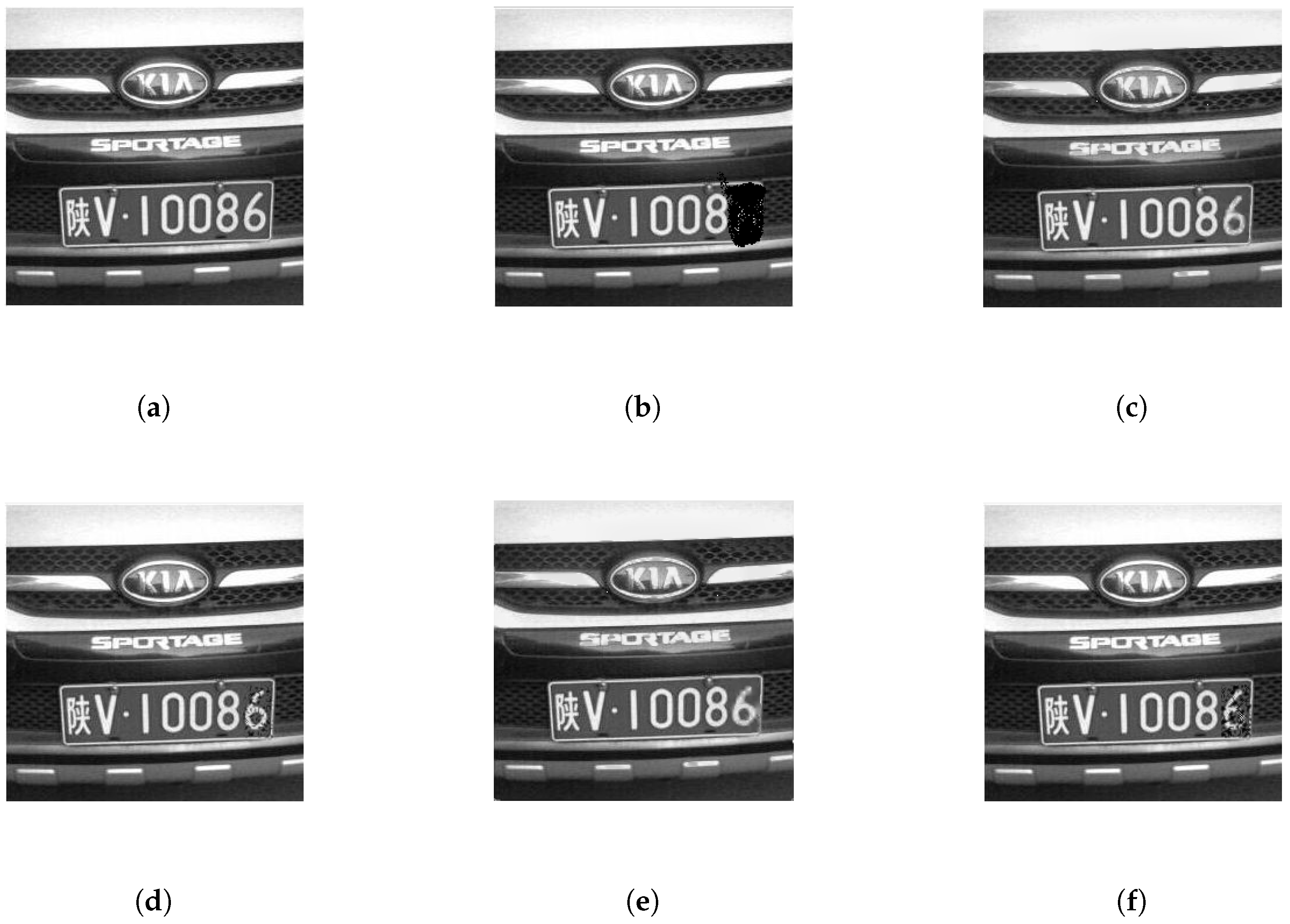
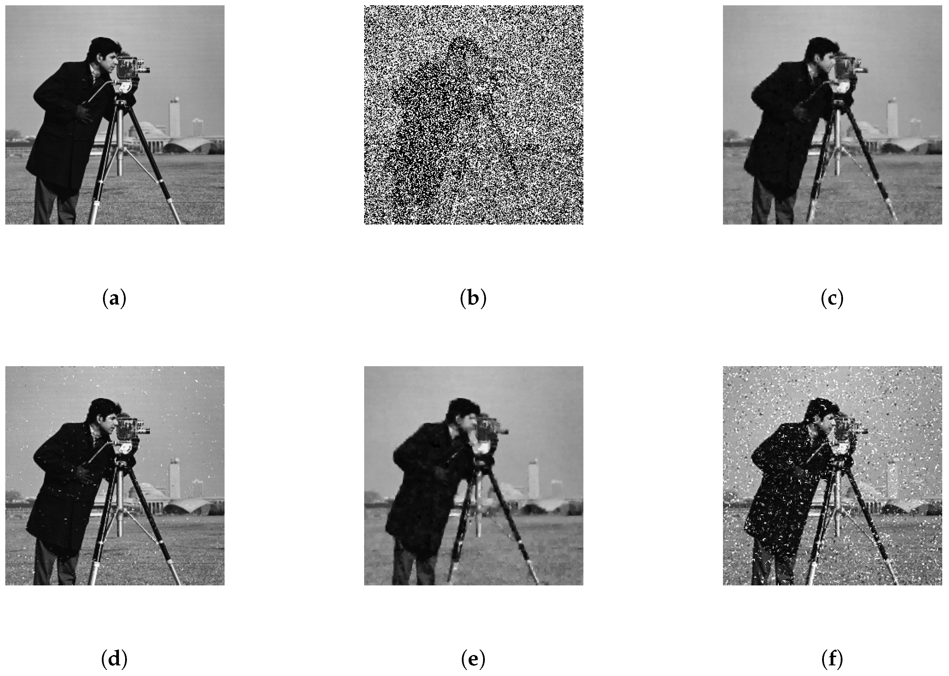
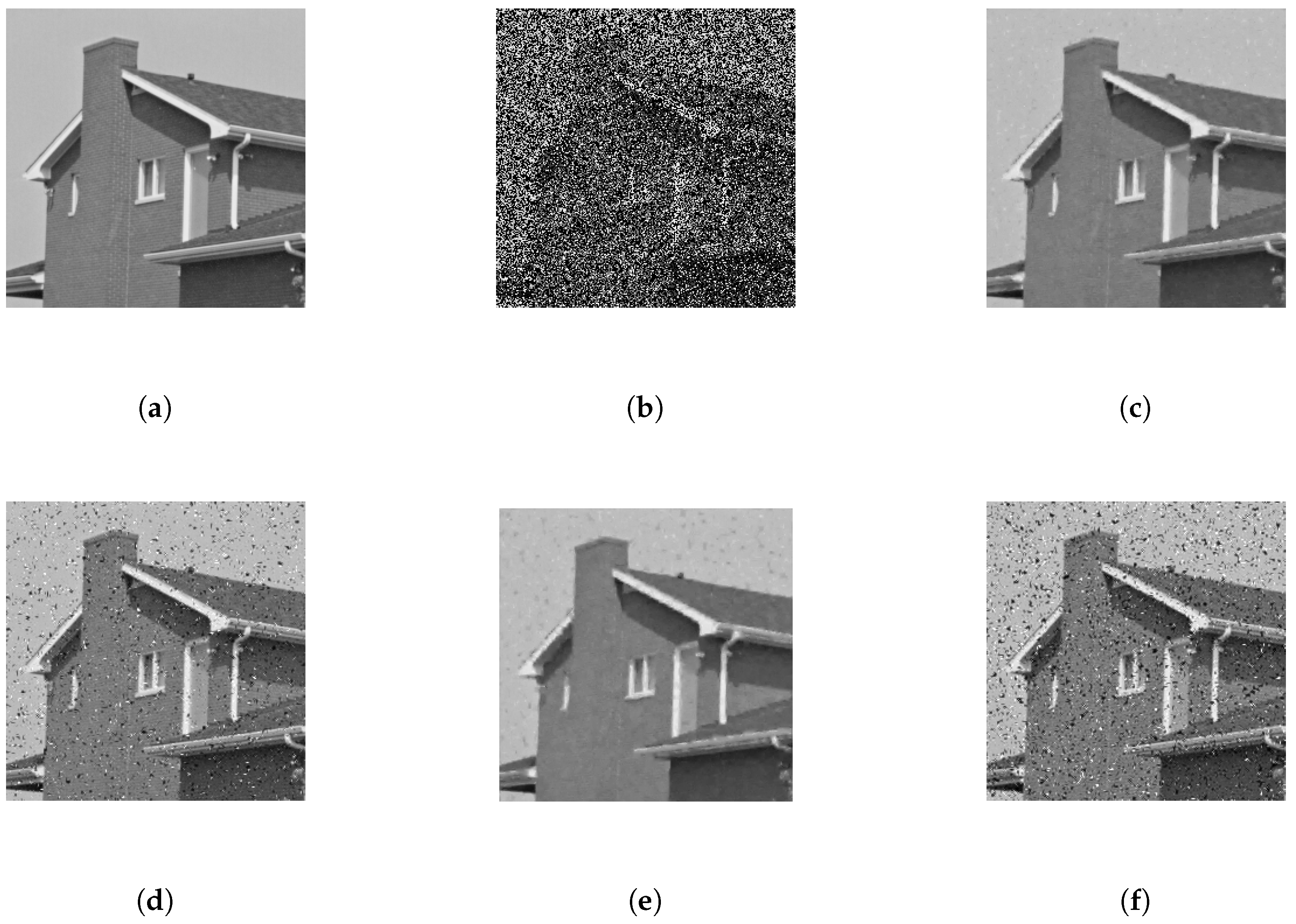
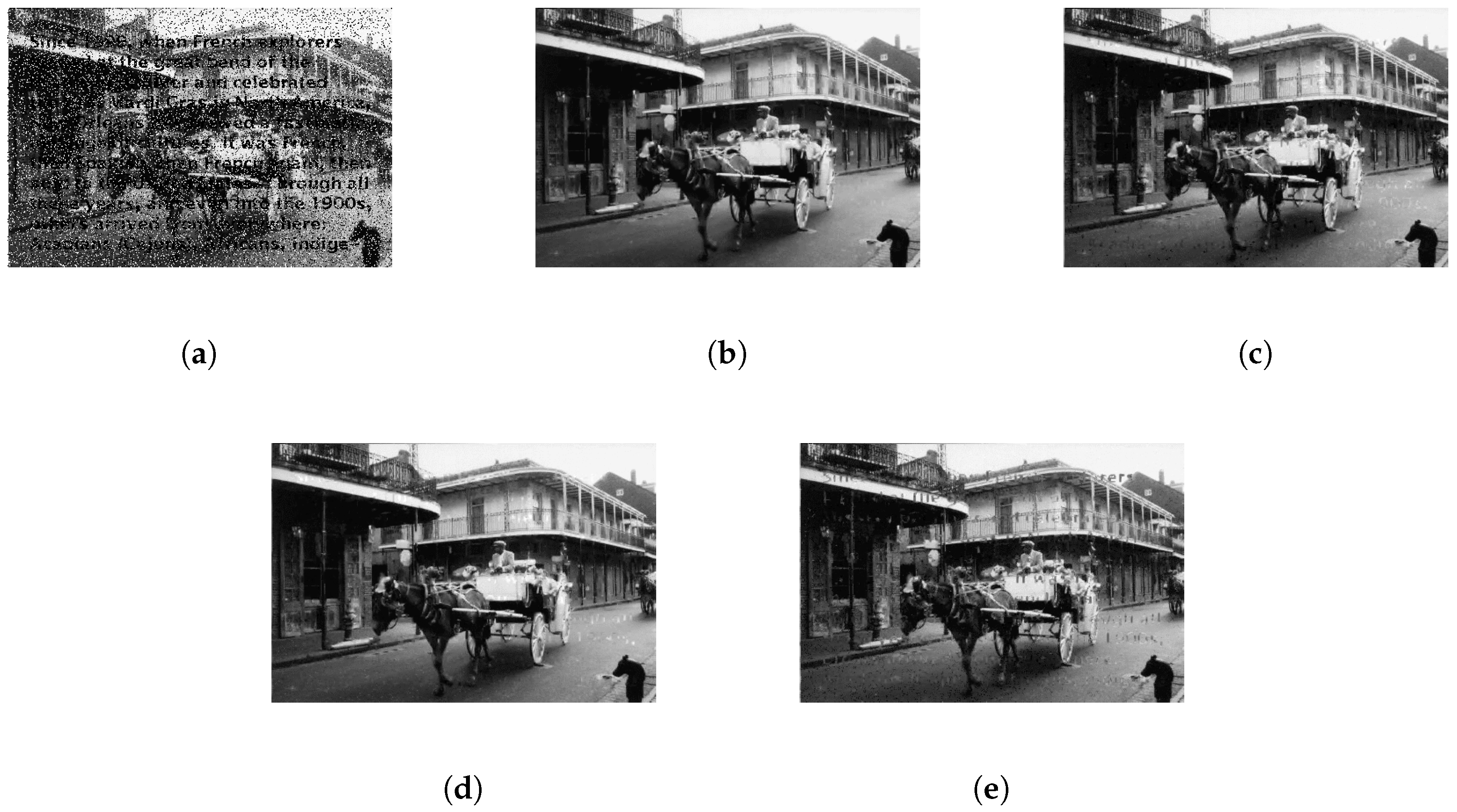
5.3. Salt-and-Pepper Noise and Data Missing

Finally, in this section, the experiments are conducted in the presence of both salt-and-pepper noise and data missing, which presents a very challenging case to recover the original image. In Figure 10b, the 40% salt-and pepper noise and the 40% data missing are utilized to corrupt the image of $\mathit{lena}$, and the restoration results obtained by the proposed methods are provided in Figure 10c–f. One observes from these figures that the framelet+APG produces a clear image with PSNR of 29.3 dB that is 22.27 dB greater than the corrupted image and 2.9 dB greater than the framelet+ADMM approach. The results of image house in Figure 11 also confirm the conclusion from the image of lena. The PSNRs, MAEs, and SSIMs under the different percentages of the noise and data missing are also provided in

Table 1. Peak signal-to-noise ratios (PSNRs) for the lena image with different levels of salt-and-pepper noise and data missing.

Salt-and-Pepper Noise+Missing	$20\%+20\%$	$30\%+30\%$	$40\%+40\%$
framelet+APG	34.42	31.57	29.26
framelet+ADMM	33.17	29.56	27.35
wavelet+APG	32.29	29.13	27.04
wavelet+ADMM	30.57	27.46	25.34

,

Table 2. Mean absolute errors (MAEs) for the lena image with different levels of salt-and-pepper noise and data missing.

Salt-and-Pepper Noise+Missing	$20\%+20\%$	$30\%+30\%$	$40\%+40\%$
framelet+APG	1.54	2.57	3.82
framelet+ADMM	2.52	3.96	5.79
wavelet+APG	4.76	7.06	10.42
wavelet+ADMM	6.23	9.87	15.43

and

Table 3. Structural similarity index (SSIMs) for the lena image with different levels of salt-and-pepper noise and data missing.

Salt-and-Pepper Noise+Missing	$20\%+20\%$	$30\%+30\%$	$40\%+40\%$
framelet+APG	0.994	0.988	0.982
framelet+ADMM	0.815	0.742	0.686
wavelet+APG	0.931	0.879	0.859
wavelet+ADMM	0.784	0.716	0.597

. Observing Table 1 reveals that, even when the corruption level is high, say 40%+40%, the highest PSNR of the reconstructed image is 29.06 dB, which is 3.92 dB greater than the lowest PSNR produced by wavelet+ ADMM. From Table 2, one observes that the MAEs obtained by the framelet+APG are the lowest under all cases, suggesting the better recovery performance, and the SSIMs obtained by the framelet+APG are always close to the one, presented in Table 3.

Finally, the proposed methods are applied to the scenario, where the data missing comes from the text imbedding into a salt-and-pepper noise corrupted image, demonstrated in Figure 12a. The reconstructed images are depicted in Figure 12b–e, where the images obtained by framelet+ADMM, wavelet+APG, and wavelet+ADMM still show the text residuals. On the other hand, the image reconstructed by framelel+ APG is satisfactory and preserves great details.

6. Conclusions

In this work, a joint estimation method of image recovery, salt-and-pepper noise suppression and data missing patter estimation are developed. Due to reformulations performed for the noise and the data missing, they are represented by the sparse signals in the time domain. This property is utilized to actively suppress the noise and perform missing pattern estimation. In order to achieve image recovery in the presence of salt-and-pepper noise and data missing, a joint estimation is developed that allows for simultaneously recovering the image, suppressing the noise, and estimating the unknown missing pattern. The resultant joint estimation is an optimization problem and it is efficiently solved by ADMM and APG based solvers. From the experiments conducted, the proposed joint estimation approach generates a significant performance improvement compared with other state-of-the-art algorithms.

References

1. Hou, L.; Liu, H.Q.; Luo, Z.; Zhou, Y.; Truong, T.K. Image Deblurring in the Presence of Salt-and-Pepper Noise. In Proceedings of the IEEE International Conference on Image Processing (ICIP 2017), Beijing, China, 17–20 September 2017. [Google Scholar]
2. Elad, M.; Aharon, M. Image denoising via sparse and redundant representations over learned dictionaries. IEEE Trans. Image Process. 2006, 15, 3736–3745. [Google Scholar] [CrossRef] [PubMed]
3. Beck, A.; Teboulle, M. Fast gradient-based algorithms for constrained total variation image denoising and deblurring problems. IEEE Trans. Image Process. 2009, 18, 2419–2434. [Google Scholar] [CrossRef] [PubMed]
4. Zhou, M.; Chen, H.; Paisley, J.; Ren, L.; Li, L.; Xing, Z.; Dunson, D.; Sapiro, G.; Carin, L. Nonparametric Bayesian Dictionary Learning for Analysis of Noisy and Incomplete Images. IEEE Trans. Image Process. 2012, 21, 130–144. [Google Scholar] [CrossRef] [PubMed]
5. Lin, T.C.; Hou, L.; Liu, H.Q.; Li, Y.; Truong, T.K. Reconstruction of single image from multiple blurry measured images. IEEE Trans. Image Process. 2018, 27, 2762–2776. [Google Scholar] [CrossRef] [PubMed]
6. Nodes, T.A.; Gallagher, N.C. Median filters: Some modifications and their properties. IEEE Trans. Acoust. Speech Signal Process. 1982, 30, 739–746. [Google Scholar] [CrossRef]
7. Zhao, Y.; Li, D.; Li, Z. Performance enhancement and analysis of an adaptive median filter. In Proceedings of the International Conference on Communications and Networking, Shanghai, China, 22–24 August 2007; pp. 651–653. [Google Scholar]
8. Zhang, P.; Li, F. A New Adaptive Weighted Mean Filter for Removing Salt-and-Pepper Noise. IEEE Signal Process. Lett. 2014, 21, 1280–1283. [Google Scholar] [CrossRef]
9. Zhang, P.; Li, F. An Efficient Adaptive Fuzzy Switching Weighted Mean Filter for Salt-and-Pepper Noise Removal. IEEE Signal Process. Lett. 2016, 23, 1582–1586. [Google Scholar]
10. Chan, T.; Wu, H. Space variant median filters for the restoration of impulse noise corrupted images. IEEE Trans. Circuits Syst. II Analog Digit. Signal Process. 2001, 10, 784–789. [Google Scholar] [CrossRef]
11. Chan, R.H.; Ho, C.W.; Nikolova, M. Salt-and-pepper noise removal by median-type noise detectors and detail-preserving regularization. IEEE Trans. Image Process. 2005, 14, 1479–1485. [Google Scholar] [CrossRef] [Green Version]
12. Ballester, C.; Bertalmio, M.; Caselles, V.; Sapiro, G. Filling-in by joint interpolation of vector fields and gray levels. IEEE Trans. Image Process. 2001, 10, 1200–1211. [Google Scholar] [CrossRef] [Green Version]
13. Rares, A.; Reinders, M.J.T.; Biemond, J. Edge-based image restoration. IEEE Trans. Image Process. 2005, 14, 1454–1468. [Google Scholar] [CrossRef] [Green Version]
14. Drori, I.; Cohen-Or, D.; Twshueun, H. Fragment-based image completion. ACM Trans. Graph. (TOG) 2003, 22, 303–312. [Google Scholar] [CrossRef]
15. Criminisi, A.; Perez, P.; Tayama, K. Region filling and object removal by exemplar-based image inpainting. IEEE Trans. Image Process. 2003, 13, 1200–1212. [Google Scholar] [CrossRef]
16. Roth, S.; Black, M.J. Fields of Experts. Int. J. Comput. Vis. 2009, 82, 205–229. [Google Scholar] [CrossRef]
17. Kwok, T.H.; Sheung, H.; Wang, C.C.L. Fields of Experts. Fast Query Ex.-Based Image Complet. 2010, 19, 3106–3115. [Google Scholar]
18. Xu, Z.; Sun, J. Image inpainting by patch propagation using patch sparsity. IEEE Trans. Image Process. 2010, 19, 1153–1165. [Google Scholar] [PubMed]
19. Mairal, J.; Elad, M.; Sapiro, G. Sparse representation for color image restoration. IEEE Trans. Image Process. 2008, 17, 53–69. [Google Scholar] [CrossRef] [PubMed]
20. Shen, B.; Hu, W.; Zhang, Y.; Zhang, Y.J. Image Inpainting via Sparse Representation. In Proceedings of the IEEE International Conference on Acoustics, Speech and Signal Processing (ICASSP 2009), Taipei, Taiwan, 19–24 April 2009. [Google Scholar]
21. Liu, H.Q.; Li, D.; Zhou, Y.; Truong, T.K. Simultaneous Radio Frequency and Wideband Interference Suppression in SAR Signals via Sparsity Exploitation in Time-Frequency Domain. IEEE Trans. Geosci. Remote Sens. 2018, 56, 5780–5793. [Google Scholar] [CrossRef]
22. Liu, H.Q.; Li, Y.; Zhou, Y.; Chang, H.C.; Truong, T.K. Impulsive noise suppression in the case of frequency estimation by exploring signal sparsity. Digit. Signal Process. 2016, 57, 34–45. [Google Scholar] [CrossRef]
23. Liu, H.Q.; Ding, D.; Li, Y.; Zhou, Y. Frequency Estimation with Missing Measurements under Impulsive Noise. In Proceedings of the IEEE 8th International Congress on Image and Signal Processing (CISP 2015), Shenyang, China, 14–16 October 2015. [Google Scholar]
24. Zorzi, M.; Sepulchre, R. AR Identification of Latent-Variable Graphical Models. IEEE Trans. Autom. Control 2016, 61, 2327–2340. [Google Scholar] [Green Version]
25. Daubechies, I.; Bates, B.J. Ten Lectures on Wavelets. J. Acoust. Soc. Am. 1992, 93, 1671. [Google Scholar] [CrossRef]
26. He, L.; Wang, Y. Iterative Support Detection-Based Split Bregman Method for Wavelet Frame-Based Image Inpainting. IEEE Trans. Image Process. 2014, 23, 5470–5485. [Google Scholar] [CrossRef] [PubMed]
27. Daubechies, I.; Han, B.; Ron, A.; Shen, Z. Framelets: MRA-based constructions of wavelet frames. Appl. Comput. Harmon. Anal. 2003, 14, 1–46. [Google Scholar] [CrossRef]
28. Sree, P.S.J.; Kumar, P.; Siddavatam, R.; Verma, R. Salt-and-pepper noise removal by adaptive median-based lifting filter using second-generation wavelets. Int. J. Signal Image Video Process. 2013, 7, 111–118. [Google Scholar] [CrossRef]
29. Daubechies, I.; Lu, J.; Wu, H.T. Synchrosqueezed wavelet transforms: An empirical mode decomposition-like tool. Appl. Comput. Harmon. Anal. 2011, 30, 243–261. [Google Scholar] [CrossRef] [Green Version]
30. Ciccone, V.; Ferrante, A.; Zorzi, M. Factor Models with Real Data: A Robust Estimation of the Number of Factors. arxiv, 2018; arXiv:1709.01168. [Google Scholar] [CrossRef]
31. Boyd, S.; Parikh, N.; Chu, E.; Peleato, B.; Eckstein, J. Distributed Optimization and Statistical Learning via the Alternating Direction Method of Multipliers. Found. Trends Mach. Learn. 2011, 3, 1–122. [Google Scholar] [CrossRef]
32. Beck, A.; Teboulle, M. A fast iterative shrinkage-thresholding algorithm for linear inverse problems. SIAM J. Imaging Sci. 2009, 2, 183–202. [Google Scholar] [CrossRef]
33. Bioucas-Dias, J.; Figueiredo, M. A new TwIST: Two-step iterative shrinkage/thresholding algorithms for image restoration. IEEE Trans. Image Process. 2007, 16, 2992–3004. [Google Scholar] [CrossRef]
Figure 1. Comparation of framelet and wavelet decomposition. (a) the lena image; (b) the sorted framelet coefficients at level 1; (c) the sorted wavelet coefficients at level 1.
Applsci 09 01426 g001
Figure 2. Restoration results of different algorithms in the case of salt-and-pepper noise only. (a) original image; (b) corrupted image with 70% salt-and-noise noise (6.95 dB); (c) reconstructed image obtained by framelet+APG (28.2 dB); (d) reconstructed image obtained by framelet+ADMM (26.5 dB); (e) reconstructed image obtained by wavelet+APG (26.1dB); (f) reconstructed image obtained by wavelet+ADMM (23.7 dB); (g) reconstructed image obtained by AM-IEPR (27.6 dB); (h) reconstructed image obtained by MED (27.3 dB); (i) reconstructed image obtained by AMF (27.4 dB). AM-IEPR: adaptive median filter and edge preserving regularization, MED: median, AMF: adaptive median filter.
Applsci 09 01426 g002
Figure 3. Results of PSNR, MAE, and SSIM at different noise levels. (a) PSNR, (b) MAE, (c) SSIM. PSNR: peak signal-to-noise ratio, MAE: mean absolute error, SSIM: structural similarity index.
Applsci 09 01426 g003
Figure 4. Restoration results of different algorithms under random data missing only. (a) original image; (b) corrupted image with 70% missing (7.23 dB); (c) reconstructed image obtained by framelet+APG (29.1 dB); (d) reconstructed image obtained by framelet+ADMM (26.7 dB); (e) reconstructed image obtained by wavelet+APG (25.9 dB); (f) reconstructed image obtained by wavelet+ADMM (23.6 dB); (g) reconstructed image obtained by BPFA (27.8 dB); (h) reconstructed image obtained by FoE (28.3 dB). FoE: fields of experts.
Applsci 09 01426 g004
Figure 5. Results of PSNR, MAE, and SSIM at different missing levels. (a)PSNR, (b)MAE, (c) SSIM.
Applsci 09 01426 g005
Figure 6. Restoration results of different algorithms under a specific data missing pattern. (a) corrupted image with 21.4% specific missing; (b) reconstructed image obtained by framelet+APG; (c) reconstructed image obtained by framelet+ADMM; (d) reconstructed image obtained by wavelet+APG; (e) reconstructed image obtained by wavelet+ADMM; (f) reconstructed image obtained by FoE.
Applsci 09 01426 g006
Figure 7. Close-up comparisons of Figure 6. (a) zoomed portion of Figure 6a; (b) zoomed portion of Figure 6b; (c) zoomed portion of Figure 6c; (d) zoomed portion of Figure 6d; (e) zoomed portion of Figure 6e; (f) zoomed portion of Figure 6f.
Applsci 09 01426 g007
Figure 8. Restoration results of different algorithms for text in Figure 6. (a) reconstructed text obtained by framelet+APG; (b) reconstructed text obtained by framelet+ADMM; (c) reconstructed text obtained by wavelet+APG; (d) reconstructed text obtained by wavelet+ADMM.
Applsci 09 01426 g008
Figure 9. Restoration results of different algorithms under specific local data missing only. (a) original image (online image); (b) corrupted image with specific local missing; (c) reconstructed image obtained by framelet+APG; (d) reconstructed image obtained by framelet+ADMM; (e) reconstructed image obtained by wavelet+APG; (f) reconstructed image obtained by wavelet+ADMM.
Applsci 09 01426 g009
Figure 10. Restoration results of different algorithms under both salt-and-pepper noise and data missing for image Cameraman. (a) original image; (b) corrupted image with 40% salt-and pepper noise and 40% missing (7.03 dB); (c) reconstructed image obtained by framelet+APG (29.3 dB); (d) reconstructed image obtained by framelet+ADMM (26.4 dB); (e) reconstructed image obtained by wavelet+APG (26.1 dB); (f) reconstructed image obtained by wavelet+ADMM (24.7 dB).
Applsci 09 01426 g010
Figure 11. Restoration results of different algorithms under both salt-and-pepper noise and data missing for image house. (a) original image; (b) corrupted image with 40% salt-and pepper noise and 40% missing (7.51 dB); (c) reconstructed image obtained by framelet+APG (31.4 dB); (d) reconstructed image obtained by framelet+ADMM (28.6 dB); (e) reconstructed image obtained by wavelet+APG (29.1 dB); (f) reconstructed image obtained by wavelet+ADMM (26.9 dB).
Applsci 09 01426 g011
Figure 12. Restoration results of different algorithms under both salt-and-pepper noise and specific data missing. (a) corrupted image with 20% salt-and-pepper and 21.4% specific missing; (b) reconstructed image obtained by framelet+APG; (c) reconstructed image obtained by framelet+ADMM; (d) reconstructed image obtained by wavelet+APG; (e) reconstructed image obtained by wavelet+ADMM.
Applsci 09 01426 g012