Article

Network Intrusion Detection Based on Novel Feature Selection Model and Various Recurrent Neural Networks

1
School of Computer Science and Engineering, Pusan National University, Busan 609-735, Korea
2
Information Technology Faculty, Hung Yen University of Technology and Education, Hung Yen 16000, Vietnam
*
Author to whom correspondence should be addressed.
Appl. Sci. 2019, 9(7), 1392; https://doi.org/10.3390/app9071392
Submission received: 24 February 2019 / Revised: 28 March 2019 / Accepted: 29 March 2019 / Published: 3 April 2019

Abstract

:
The recent increase in hacks and computer network attacks around the world has intensified the need to develop better intrusion detection and prevention systems. The intrusion detection system (IDS) plays a vital role in detecting anomalies and attacks on the network which have become larger and more pervasive in nature. However, most anomaly-based intrusion detection systems are plagued by high false positives. Furthermore, Remote-to-Local (R2L) and User-to-Root (U2R) are two kinds of attack which have low predicted accuracy scores in advance IDS methods. Therefore, this paper proposes a novel IDS framework to overcome these IDS problems. The proposed framework including three main parts. The first part is to build SFSDT model which is the feature selection model. SFSDT is to generate the best feature subset from the original feature set. This model is a hybrid Sequence Forward Selection (SFS) algorithm and Decision Tree (DT) model. The second part is to build various IDS models to train on the best-selected feature subset. The various Recurrent Neural Networks (RNN) are traditional RNN, Long Short-Term Memory (LSTM), and Gated Recurrent Unit (GRU). Two IDS datasets are used for the learned models in experiments including NSL-KDD in 2010 and ISCX in 2012. The final part is to evaluate the proposed model by comparing the proposed models to other IDS models. The experimental results show the proposed models achieve significantly improved accuracy detection rate as well as attack types classification. Furthermore, this approach can reduce the computation time by memory profilers measurement.

1. Introduction

Computer networks have developed rapidly over the years, significantly contributing to social and economic development. International trade, healthcare systems, and military capabilities are examples of human activities that increasingly rely on computer networks. This has led to an increasing interest in network security from research and industries. The main role of IDSs is critical since the networks can be vulnerable to be attacked by both internal and external intruders [1,2]. The IDS has become one of the fundamental components of computer security to detect these malicious threats with the aim of protecting systems from common harms and group vulnerabilities [3].
IDS is to create systems that do not need expert knowledge to create and update signatures but rather learn and update themselves. For example, the system should have low false positive rates to make practice for deployment in a live network environment to improve network security. The goal of intrusion detection is to identify preferably in real time, the unauthorized use, misuse, and abuse of computer systems by both system insiders and external penetrators [4]. The intrusion detection problem is becoming more challenging due to the significant increase in computer network connectivity, the speed of technological advancement, and the ease of finding hackers for hire. Thus, IDSs are security systems used to monitor, recognize, and report malicious activities or policy violations in computer systems and networks. However, the false recognition of IDS results in that it is difficult for network administrators to deal with intrusion reports. These IDSs rely on the signatures of known attacks. Human independent IDSs that incorporate machine learning techniques have been developed as a solution to solve this problem. Besides, machine learning IDSs learn from normal and abnormal traffic by training on a dataset in order to predict an attack by using classification. Several machine learning techniques have been successfully implemented as classifiers on IDSs, but they have numerous flaws such as low throughput and high false detection rates [5,6,7,8].
Another challenge in IDS is the different attack types including Probe, R2L, U2R, and Denial-of-Service (DoS) should be detected well by IDS techniques. However, one of the most difficult attacks to detect is R2L attack because it related to the host level features and network level. Besides, U2R attack is also hard to detect at an early stage because it involved the semantic detail such as content-based and target an application. This becomes one challenge in IDS techniques. Presently, IDSs are generally categorized as signature-based (misuse detection) systems, behavior-based (anomaly detection) systems, or hybrid systems. Misuse IDSs are commonly deployed in practical networks since they are robust or low false alarm rate (FAR). However, the main shortcoming is their inability to detect new attacks. Current research is focused on the anomaly detection approach since it can detect new attacks. However, these approaches suffer from high false positive rates leading to impractical implementation in live network settings.
On the other hand, neural networks have been employed in anomaly detection to identify whether the behaviour of data is normal or abnormal. This network can detect both known and unknown attacks with moderate performance. Several researchers have focused on developing IDSs based on deep networks. However, a robust deep network model is how to estimate or optimize its parameters as effectively. This model designing is one of the challenges derived from high-dimensional data leading to the curse of dimensionality phenomenon. In order to avoid this issue, input patterns need to be reduced the dimensionality. This method can also reduce the amount of required computation. Although conventional techniques are projection-based such as Principal Component Analysis (PCA) (unsupervised method) or Linear Discriminant Analysis (LDA) (supervised method), feature selection techniques are considered as promising alternatives.
Feature selection methods are designed to deal with the combinatorial search problem. These methods require a search strategy to select candidate subsets which are evaluated by an objective function. A search strategy is therefore needed to direct the feature subset selection process as it explores the space of all possible combination of features. The object function evaluates candidate subsets and returns a measure of their goodness, a feedback signal used by the search strategy to select new candidates. These new candidates are fewer features mean fewer parameters for pattern recognition. They enable improving generalization capabilities, computation complexity, and execution time. Thus, this work proposes a feature selection model to reduce high dimensional data. By this way, an IDS framework based on deep neural networks is applied to the result of the proposed feature selection model to improve accuracy performance as well as reduce FAR. Besides, this propose can detect attack types well, especially U2R and R2L attacks. The proposed algorithm is evaluated on two IDS datasets including NSL-KDD and ISCX datasets.
The rest of this paper is organized as follows. Section 2 presents related works. Section 3 presents the proposed IDS framework. Section 4 shows the experiment results and discussion. The conclusions are presented in Section 5.

2. Related Work

Traditionally, the researchers study intrusion detection approaches from two major perspectives: anomaly detection and misuse detection. However, there is no significant difference between these two approaches. Stavrouslakis and Stamp [9] proposed a classification system to further divide these approaches into three subcategories, including computation dependent on approach, artificial intelligence, and biological concepts. However, such a classification makes it too hard to see the whole properties of detection approaches. Although there is a lack of more detailed views for detection approaches, Liao et al. [10] proposed a classification system consisting of five sub-classes with an in-depth perspective on their characteristics: statistics-based, pattern-based, rule-based, state-based, and heuristic-based. These sub-classes belongs to intrusion detection based on machine learning methods.
  • The researchers who applied statistic-based classification in IDSs include ANFIS-IDS (Mar et al. [11]), distance-based (Sabahi and Movaghar [12]), Bayesian-based (Stavrouslakis and Stamp [9]), and game theory (Li et al. [13]). Nevertheless, these technique’s characteristics are simple but less accuracy, self-study, and poor control.
  • Pattern-based classification consists of pattern matching (Karti el al. [14]), petrinet (Lazarevic el al. [15]), keystroke monitoring (Murali and Rao [16]), and file system checking (Lazarevic et al. [15]). However, these techniques are simple but less flexible, using user’s typing pattern.
  • Rule-based classification includes rule-based (Modi et al. [17]), data mining (Xie et al. [18]), model/profile-based (Kartit el al. [14]), and support vector machines (SVMs) (Kolias et al. [19]). However, these methods are not easily created and updated; automatically generated models.
  • State-based classification includes state-transition analysis (Sabahi and Movaghar, [12]), user intention identification (Lazarevic el al. [15]), Markov process model (Li et al. [13]), and protocol analysis (Stavroulakis and Stamp [9]). However, the characteristics of these techniques are high-level task pattern, probabilistic, self-training, low false positive rate, and less effective.
  • Heuristic-based classification includes neural networks (Modi et al. [17]), fuzzy logic (Mar et al. [11]), genetic algorithm (Garcia Teodoro el al. [20]), immune system (Lazarevic el al. [15]), and swarm intelligence (Alomari and Othman [21]). Self-learning, fault tolerant, configurable, scalable, flexible are characteristics of these techniques.
Currently, deep learning has become more attractive and effective in IDS field. Generative learning and discriminative learning are two kinds of deep networks.
First, generative learning in deep networks intends to capture high-order correlations between observed or visible data for pattern analysis or synthesis when no available information about target class labels. B. Abolhasanzadeh [22] proposed an approach to detect attacks on big data using a deep autoencoder. The experiment was conducted on the NSL-KDD dataset to test the method of applying bottleneck features in dimensionality reduction as part of intrusion detection. The obtained results were more accurate than PCA, factor analysis, and Kernel/PCA with 95.25% for train data and 95.06% for test data. However, the authors did not mention about accuracy every single attack type. Besides, U. Fiore et al. in [23] explored the use of a deep Boltzmann machine (DBM) in anomaly detection by training a network with real-world data traces from 24 h workstation traffic. This experiment tested the accuracy of DBM in classifying normal data and data infected by the bot. A second experiment trained DBM with KDD Cup’99 dataset and tested it against real-world data. The result obtained 84% accuracy on KDD Cup dataset. Z. Alom et al. [24] also exploited the deep belief network (DBN) capabilities to detect intrusion through a series of experiments. The authors trained DBNs with NSL-KDD data to identify unknown attacks. They concluded that DBN was a good IDS based on an accuracy of 97.5% achieved in the experiment. This result was compared with existing DBN-SVM and SVM classifiers which the DBN outperformed. However, the authors did not mention the classification performance type of attacks. The ability of the Jordan RNN to store information in neurons allows it to train fewer input vectors for more accurate classification of normal and abnormal patterns [25]. The author also did not mention about accuracy and only suitable for online real-time applications.
Second, discriminative learning in deep neural networks depends on the observed data while learning how to do the classification. Target label data are always available in direct or indirect forms. Thus, it is considered to be supervised learning. RNNs and convolutional neural networks are two types of discriminative architectures. LSTM RNN [26] and LSTM with Nadam optimizer [27] are applied on the KDD Cup’99 dataset. The detection accuracy rates were high with 96.93% and 97.54% corresponding to LSTM RNN and LSTM with Nadam optimizer models. However, the FARs of these models were still slightly higher than other models obtained at 10.04% and 9.98%, respectively. However, the researchers [28] mentioned these methods as well as generative learning.

3. The Proposed IDS Framework

The proposed IDS framework is shown in Figure 1. This architecture includes four steps. The first step is to preprocessing from the original dataset. The second step is to generate feature subsets by SFS. Then, accuracy and error scores are measured corresponding to each subset generated based on a machine learning model. This machine learning model is Decision Tree (DT). In this work, the task of DT is to predict accuracy and loss scores for each combined feature. After that, the best feature subset is chosen based on the maximum accuracy score. In the third step, IDS classifiers are built for learning the best-selected subset feature data. The final step is to evaluate various IDS RNNs models based on two things. The first task is the comparison with other IDS classifiers. The second is measurement memory profilers of the proposed models.
Preprocessing dataset. This is the first step in the IDS framework. In ISCX dataset, XML files with data labeled as input data are chosen. Then, the following procedures are performed: (1) converting XML files to CSV files; (2) splitting *.CSV files data into training and testing data. In NSL-KDD dataset, the NULL values are solved by using imputation technique. This technique is used to replace missing data with substituted value.
SFSDT model. The purpose of this component is to select the best feature subset from the complete feature set from the original datasets.
In mathematics, given a feature set x = x i | i = 1 n , find a subset x m = x i 1 , x i 2 , , x i m , with  m < n , that optimizes an criterion function (CF), ideally the probability of correct classification (see Figure 2).
The first goal of the presented feature selection algorithms is to reduce the feature space D = x 1 , x 2 , , x n to a subset of features D n in order to improve or optimize the computational performance of the classifier and avoid the curse of dimensionality. The second goal is to select a sufficiently reduced subset from the feature space D without significantly reducing the performance of the classifier. An optimal feature subset of size m is chosen by C F . C F is typical, simply, and intuitively assesses the recognition rate of the classifier.
This work proposes a model feature selection by hybrid SFS algorithm and DT model because of some reasons as follows.
SFS [29] is the simplest greedy search algorithm which is a bottom-up search procedure. SFS starts with an empty feature subset and sequentially adds features from the whole input feature space to this subset until the subset reaches a desired (user-specified) size. For every iteration which is the inclusion of a new feature, the whole feature subset is evaluated which is expected for the features that are already included in the new subset. The evaluation is done by the so-called CF which assesses the feature that leads to the maximum performance improvement of the feature subset if it is included.
Besides, DT [30] is a classical and well-known in the machine learning model. DT model has the main different somehow is about the domain of application. While some models like KNN (K-Nearest Neighbour), SVM etc. are used for continuous value input, DT is applicable for continuous and categorical input (discrete values) with high accuracy classification. In NSL-KDD and ISCX datasets, the input features are discrete values. Besides, NSL-KDD data contains multi-output values (with four attack types). The DT model can handle a multi-output problem. In the proposed method, this work adjusted and replaced a simple CF function in SFS algorithm by accuracy and error scores of DT model on each feature subset is generated by SFS. Based on the accuracy and error scores, this proposed method can decide and choose the best feature subset from the original feature set. In summary, the goal of SFSDT is a feature selection based on the learning model. This proposed model can solve the high-dimensional data leading to the curse of dimensionality phenomenon in big data. The main reason reduces accuracy performance prediction because of this problem. In order to solve this issue, input patterns need to be reduced the dimensionality.
SFSDT Algorithm 1 is started from the empty set, sequentially add the features x + that results in the highest accuracy score of the DT model. The accuracy of the DT model on the validation dataset (feature subset) is the maximum value. This reduces the number of features which is likely due to a decrease of the curse of dimensionality.
Algorithm 1 The pseudocode of the proposed SFSDT algorithm
Require: 
Y d , o u t p u t _ c l a s s  
Ensure: 
Y k , accuracy_scores, error_scores  
1:
accuracy_scores = []  
2:
error_scores = []  
3:
d is the number of complete feature  
4:
Start with the empty set Y 0 =  
5:
Select the next best feature x + = a r g m a x [ a c c u r a c y ( Y k + x + ) ]  
6:
accuracy = Accuracy score of DT model on ( x + , o u t p u t _ c l a s s )  
7:
error = Error of DT model on ( x + , o u t p u t _ c l a s s )  
8:
accuracy_scores.append (accuracy)  
9:
error_scores.append (error)  
10:
Update Y k + 1 = Y k + x + ; k = k + 1  
11:
Go to step 5  
12:
Termination k = d  
13:
return Y k , accuracy_scores, error_scores
  • Input. The input of SFSDT algorithm is the set of all features, denoted by Y = y 1 , y 2 , , y d and the output of class data is the type of each attach in each dataset, denoted by o u t p u t _ c l a s s . The SFSDT algorithm takes the whole d-dimensional feature set as input. The o u t p u t _ c l a s s is actual output which used in DT model to compare the predicted class of DT model. After that, DT can measure accuracy and error scores corresponds to each subset feature generated.
  • Output. Feature subsets, accuracy_scores, and error_scores are output values. Feature subset is denoted by Y k , Y k = y j | j = 1 , 2 , , k , where k = ( 0 , 1 , 2 , , d ) . The algorithm returns a subset of the feature space of a specified size k, where k < d , has to be specified a prior.
  • Initialization. Initialization of the algorithm with an empty set Y 0 = , so that k = 0, where k is the size of the subset.
  • Searching procedure. Adding an additional feature x + to the feature subset Y k . x + is the feature that maximizes the criterion function. accuracy is the criterion function with the best classifier performance of DT model if it is added to Y k . Hence, the best feature subset is contained in Y k . This process is repeated until reaching the termination criterion.
  • Termination. Termination is stopped when k equal to the number of combination desired features. The new feature subset Y k are added until the feature subset of size k contains the number of desired feature d that specified a prior.
Various RNNs.
  • Traditional RNN model
    RNN is a traditional recurrent neural network incorporates either supervised learning or unsupervised learning. This model has an input sequence data whole length could be as large as its depth. The RNN model architecture consists of a feedback loop that links each layer with the ability to store data of the previous input. Thus it can increase the reliability of the model. Elman and Jordan RNNs are two types of RNN model. While the Elman model has a simple feedback loop in each layer, the Jordan model has a feedback loop for all neurons within a layer to the next layer. There is also a feedback loop connecting a neuron to itself. RNNs are recurrent because they perform the same task for each element in a sequence, with the output is dependent on the previous computations. In other words, the RNN is a memory that captures the information that has been computed so far. The structure of an RNN is shown in Figure 3.
    In this model, x ( t ) is input layer at time t with index i. h ( t 1 ) is hidden layer at time t 1 with index s. h ( t ) is hidden layer at time t with index j. y ( t ) is output layer at time t with index e. U is weight matrix connects input to hidden layer with index i , j . W is weight matrix connects previously hidden to hidden layer with index s , j . V is weight matrix connects hidden to output layer with index j , e . m is number of input units. n is number of hidden units. k is number of output units. The formulas that govern the computations in an RNN are as follows.
    In the first step, h ( t ) is calculated based on the previously hidden state and the input at the current step:
    h ( t ) = f ( U x ( t ) + W h ( t 1 ) )
    where f is a nonlinear function such as t a n h or R e L U . h ( t 1 ) is required to calculate the first hidden state which is typically initialized to all zeroes. In the second step, y ( t ) is the output at step t is calculated following the formula:
    y ( t ) = f ( V h ( t ) )
    In RNNs, h j ( t ) and y e ( t ) are calculated for recurrent networks as follows:
    h j ( t ) = f ( Σ i m x i ( t ) u i j + Σ s n h s ( t 1 ) w s j )
    y e ( t ) = f ( Σ j = 1 k h j ( t ) v j e )
    RNN training is similar to train a traditional neural network. This model also used the backpropagation algorithm but with a slight difference. Because the parameters are shared by all time steps in the network, the gradient at each output depends not only on the calculations of the current time steps but also the previous time steps. This is called backpropagation through time (BPTT) [31]. Unfortunately, vanilla RNNs trained with BPTT have difficulty learning long-term dependencies because of the so-called vanishing/exploding gradient problem [32]. There are some machines that deal with these problems, and certain types of RNNs (like LSTMs, GRUs) were specifically created to get around them.
  • LSTM model
    LSTM is proposed by Hochreiter and Schmidhuber [33]. This model is more capable to learn long-term dependences model than traditional RNN model. Thus the network overcomes the vanishing gradient problem. Furthermore, this network was designed to be better at storing and accessing information compared to standard RNNs. The memory cells replaced the hidden notes in traditional RNNs. A memory cell includes three gates: an input gate i t , a forget gate f t , and an output gate o t . The memory cell also are known as a cell state c t . The incoming signals can alter the cell state or block it by the input gate. The cell state has an effect on other neurons or prevents it from doing so by the output gate. Modulate the cell state of the memory cell can allow the cell to remember or forget its previous state as need by the forget gate.
    In LSTM networks, the hidden units are replaced by LSTM cells. Figure 4 shows the architecture of this model which has two input units, three LSTM cells as hidden units, and three output units. Assumption that X t = [ x t 1 , x t 2 , , x t n x ] is an input vector. H t = [ h t 1 , h t 2 , , h t n h ] is hidden vector. Y t = [ y t 1 , y t 2 , , y t n y ] is output vector. C t = [ c t 1 , c t 2 , , c t n c ] is cell vector. The elements of each vector are corresponding units for each layer of the LSTM model. n x , n h , n c , and n y are the numbers of input, hidden, cell, and output units, respectively. σ is the s i g m o i d function. W t x i , W t x f , W t x c , and W t x o are weight metrics that connect from the input node to the input gate, forget gate, cell state, and output gate, respectively. W t h i is a weight matrix that connects from the hidden node (LSTM cell) to the input gate. W t h f is a weight matrix that connects from the LSTM cell to the hidden gate. W t h c is a weight matrix that connects from the LSTM cell to the cell gate. W t h o is a weight matrix that connects from the LSTM cell to the output gate. W t c o is a weight matrix that connects from the cell state to the output node. W t h y is a weight matrix from the LSTM cell to the output node. There are several steps to calculate values of each layers.
    The first step, the decision is what information is to be thrown away from the cell state by a s i g m o i d ( σ ) layer called the forget gate.
    f t = σ ( W t x f Σ i = 1 n x x t i + W t h f Σ j = 1 n h h t 1 j + W t c f Σ k = 1 n c c t 1 k )
    The second step, the decision is what new information is going to be stored in the cell state by two processing. First one is to decide which values to by update by the input gate. The second one is a vector of new candidate value c t is created by the t a n h layer.
    i t = σ ( W t x i Σ i = 1 n x x t i + W t h i Σ j = 1 n h h t 1 j + W t c i Σ k = 1 n c c t 1 k )
    c t = f t c t 1 + i t t a n h ( W t x c Σ i 1 n x x t i + W t h c Σ j = 1 n h h t 1 j )
    The final step, the output is calculated based on the cell state. The value of the output gates is computed and used it for the memory block output
    o t = σ ( W t x o Σ i = 1 n x x t i + W t h o Σ j = 1 n h h t 1 j + W t c o Σ k = 1 n c c t 1 k )
    h t = o t t a n h ( c t )
    The output units y t are computed with hidden vector h t
    y t = σ ( W t h y Σ i = 1 n h h t i )
  • GRU model
    A slightly more dramatic variation on the LSTM is GRU, introduced by Cho, et al. [34] in 2014. This model combines the forget gate and input gate into a single update gate. It also merges the cell state and hidden state and makes some other changes. The resulting model is simpler than standard LSTM models and has been growing increasingly popular. A GRU has two gates, a reset gate r t , and an update gate z t . Intuitively, the reset gate determines how to combine the new input with the previous memory, while the update gate defines how much of the previous memory to keep around. The basic idea of using a gating mechanism to learn long-term dependence is the same as in an LSTM. The assumption that the GRU model has two input units, and three GRU units are presented in Figure 5.
    Similar to LSTM model, X t , H t , and Y t are the input vector, hidden vector, and output vector, respectively. W t x z , W t x r and W t x H are weight matrices from the input layer to the update gate, the reset gate, and the hidden state, respectively. W t h z , W t h r , and W t h H are weight matrices from the hidden layer to the update gate, the reset gate and the hidden state, respectively. W t h is the weight matrix from the hidden unit to the output.
    In the first step, the update gate z t at time t is calculated as follows:
    z t = σ ( W t x z Σ i = 1 n x x t i + W t h z Σ j = 1 n h h t 1 j )
    In the second step, the reset gate r t is calculated:
    r t = σ ( W t x r Σ i = 1 n x x t i + W t h r Σ j = 1 n h h t 1 j )
    In the third step, the hidden state H t is calculated:
    H t = t a n h ( W t x H Σ i = 1 n x x t i + W t h H ( r t Σ j = 1 n h h t 1 j ) )
    Finally, the value of the memory block, output h t is computed using H t
    h t = ( 1 z t ) * h t 1 + z t * H t
    In order to compute the output units in the output layer, the output units y t of the GRU model is computed with hidden vector h t
    y t = σ ( W t h Σ i = 1 n h h t i )
Evaluation performance IDS classifiers. This step is to evaluate the performance of the proposed IDS framework. The performance evaluation is based on two things. The first is comparison accuracy of the proposed IDS models to advance IDS models. The second is measurement memory profiler of the proposed IDS model on the complete feature set and the best-selected feature subset. In the experiment, confusion matrix and receiver operating characteristic (ROC) are used to measure multi-attack output. Besides, memory used and time executed are measured in memory profiler.
  • Confusion matrix is presented in Figure 6. The classifier’s goal is to identify as many TPs and TNs as possible while FPs and FNs need to reduce.
    where True positive (TP) is an attack that is correctly classified as an intrusion; True negative (TN) normal traffic correctly classified as normal traffic; False positive (FP) is when normal traffic is classified as an intrusion; False negative (FN) is when an intrusion that is classified as normal traffic.
  • ROC curve is a two-dimensional graph in which the false positive rate is plotted on X-axis and the true positive rate is plotted on the Y-axis. The ROC curves are useful to visualize and compare the performance of classifier methods. Figure 7 shows the ROC curves example for multi-classes classification (10 classes).
    True Positive Rate (TPR) and False Positive Rate (FPR) are calculated as following formulas:
    T P F = T P T P + F N
    F P R = F P F P + T N
  • Memory profiler is a python module for monitoring memory consumption of a process as well as line-by-line analysis of memory consumption for python programs. In this work, memory profiler library (https://github.com/pythonprofilers/memory_profiler) is used to calculated time-based memory usage of the proposed models. Memory usage a long time is executed and recorded via a command line such mprof run <script>, where <script> is the Python script. The final step is to visualize the result of time-based memory usage via command line mprof plot. The result of memory profiler example is plotted in Figure 8.

4. Experiment Results and Discussion

This section points out the experiment results and discussion of the approach to build the efficient IDS classifier based on proposed SFSDT model. Three experiments are shown in detail in Section 4.2. Via the experiment result, the best IDS classifier is determined. Next, the evaluation of the proposed method is discussed in Section 4.3.

4.1. Dataset Description

NSL-KDD dataset (http://www.unb.ca/research/iscx/dataset/iscx-NSL-KDD-dataset.html) [35] is a new version of KDD Cup’99 dataset. The KDD Cup’99 contains train and test sets which are duplicated about 78% and 75% of the records, respectively. Thus, NSL-KDD dataset was redundant records in the train set and no duplicate records in new test sets. Besides, this dataset still remains 41 input features and 1 output feature. The input features include [duration, protocol_type, service, flag, src_bytes, dst_bytes, land, wrong_fragment, urgent, hot, num_failed_logins, logged_in, num_compromised, root_shell, su_attempted, num_root , num_file_creations, num_shells, num_acces_files, num_outbound_cmds, is_host_login, is_guest_login, count, srv_count, serror_rate, srv_serror_rate, rerror_rate, srv_rerror_rate, same_sr_rate, diff_srv_rate, srv_diff_host_rate, dst_host_count, dst_host_sr_count, dst_host_same_srv_rate, dst_host_diff_srv_rate, dst_host_same_src_por_rate, dst_host_srv_diff_host_rate, dst_host_serror_rate, dst_host_srv_serro_rate, dst_host_rerror_rate, dst_host_srv_rerror_rate]. The output name is [Attack]. The output value consists of [ ’Normal’, ’R2L’, ’DoS, ’U2R’, ’Probe’]. As a result, several records in train and test sets are reasonable which makes it affordable to run the experiments on the complete set without the need to randomly select a small partition. The experiment uses KDDTest+ dataset file in learned models.
In ISCX dataset (http://www.unb.ca/cic/research/datasets/ids.html), the real-life dataset was created by collecting network traffic data for several consecutive days. ISCX in 2012 is a real-life dataset that builds on the concept of profiles which include details on intrusions. This dataset is created by Shiravi Ali, et al. [36]. This dataset was designed specifically for developing, testing, and evaluating network intrusion and anomaly detection algorithms. It uses two profiles, α and β , during the generation of the datasets. The α profiles were constructed using the knowledge of specific traces. Real packet traces were analyzed to create α and β profiles for agents that generated real-time traffic for HTTP, SMTP, SSH, IMAP, POP3, and FPT protocols. Various multi-stage attack scenarios were explored to generate malicious traffic. This dataset consists of seven days of network activities, both normal and malicious. A pcap extension file (.*pcap) and XML extension file (.*xml) are two extension files.
In data preparation, the ready-made training and testing datasets are not available in the original dataset, and it is difficult to perform experiments on huge data (*.pcap files). Hence, the file “labelled_flows_xml” which contained flow information in XML format for each day are used. Furthermore, the labeled flow file supports the use of supervised machine learning algorithms. The flows were generated using IBM WRadar appliance. The flow file was labeled with “Normal” and “Attack”. The [Tag] feature indicates whether the flow is normal or part of an attack scenario. However, all flows from day 1–Friday (11 June 2010) were normal; therefore no flow XML file was included. The XML files contained 19 attributes for input values and one attribute for the output value. The attributes for each day data file include [appName, totalSourceBytes, totalDestinationBytes, totalDestinationPackets, totalSourcePackets, sourcePayloadAsBase64, sourcePayloadAsUTF, destinationPayloadAsBase64, destinationPayloadAsUTF, direction, sourceTCPFlagsDescription, destinationTCPFlagsDescription, Source, protocolName, sourcePort, destination, destinationPort, startDateTime, stopDateTime, Tag].
In the preprocessing dataset, the *.XML file is read and converted to *.CSV file. Each attribute in the XML file is a column in the CSV file. The [Tag] feature is the output which contains target values. The other features are input features as well as input values. A cross-validation technique is used to split the preprocessing dataset that randomly followed the ratio of 75% and 25%, respectively. Table 1 presents a description of the number of training and testing data of ISCX dataset.
Further adjustments were made to make the data fit for use. Reduction of the number attributes from all the possible attributes have to be carried out. The following attributes were chosen for the experiment: [appName, totalSourceBytes, totalDestinationBytes, totalDestinationPackets, totalSourcePackets, direction, sourceTCPFlagsDescription, destinationTCPFlagsDescription, source, protocolName, sourcePort, destination, destinationPort, startDateTime, stopDateTime, Tag]. Some accumulative or redundant attributes such as [sourcePayloadAsBase64, sourcePayloadAsUTF, destinationPayloadAsBase64, destinationPayloadAsUTF] were removed.

4.2. Experiment Results

Three experiments on NSL-KDD and ISCX datasets are performed. These experiments are implemented on Windows 10 and used Python language.
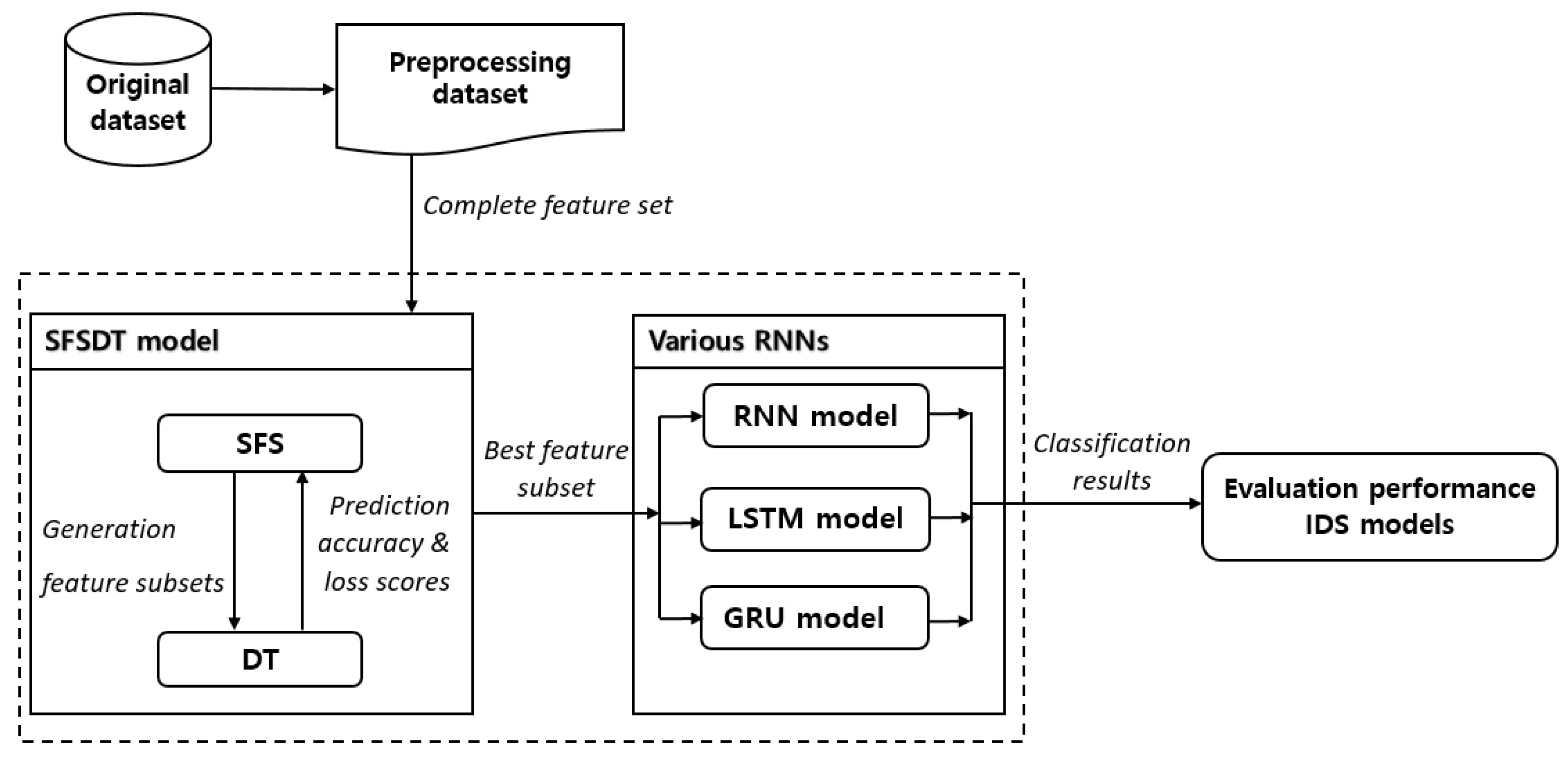
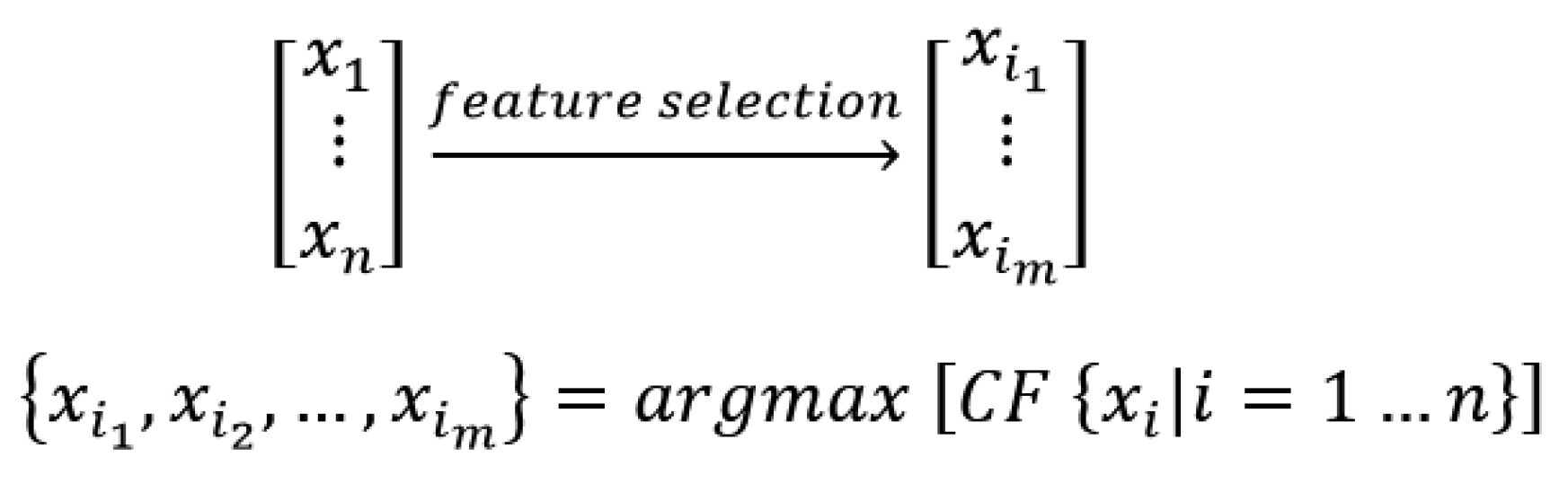
  • The first experiment is to build SFSDT model to generate the best feature subset on both IDS datasets. The proposed model can generate the list of combination feature subsets. The best feature subset is selected based on the best score of accuracy and error.
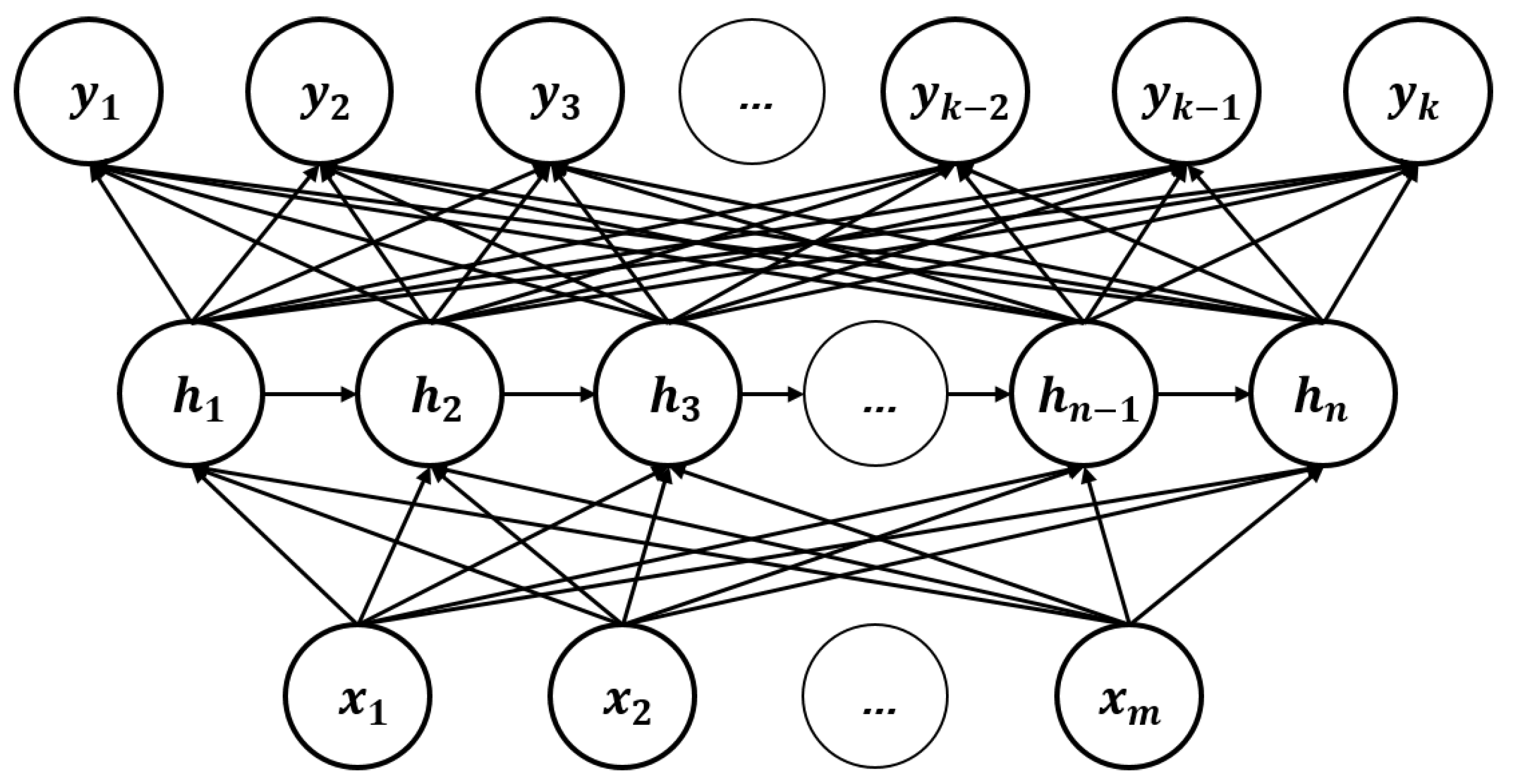
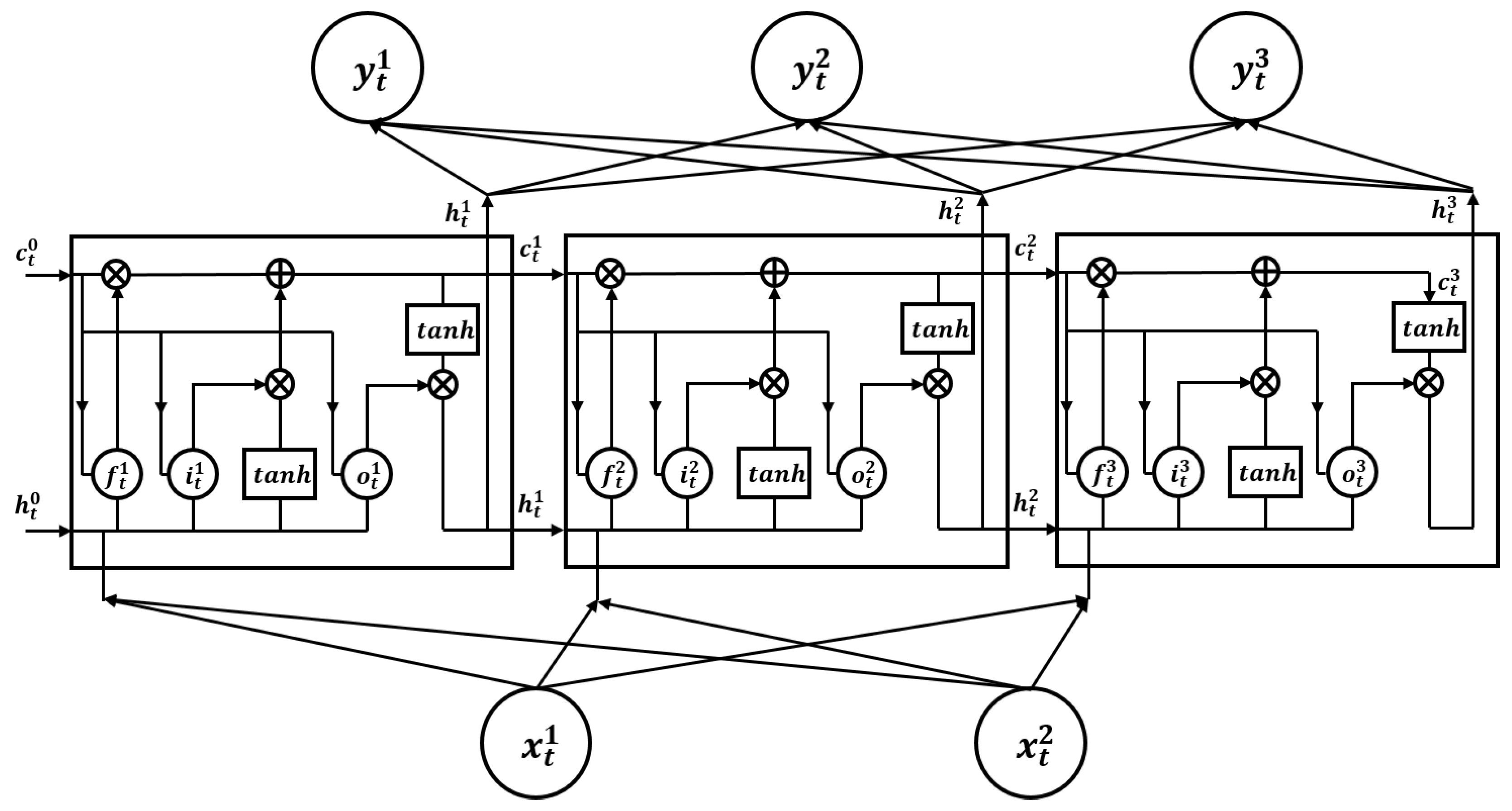
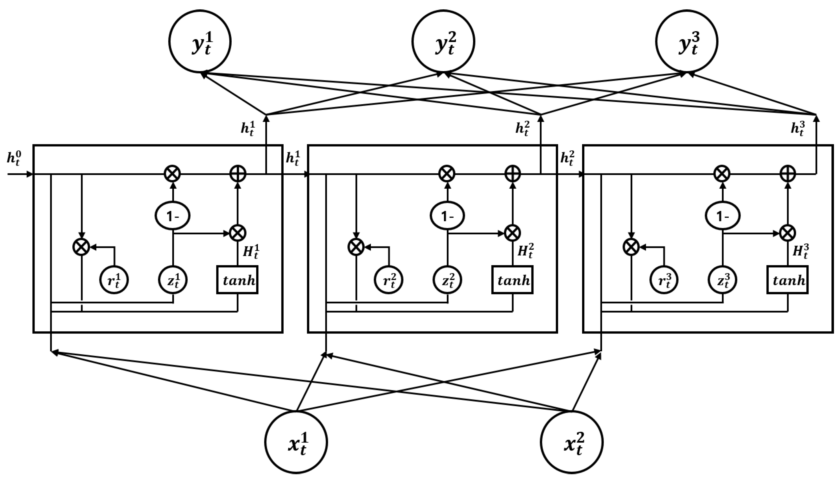
  • The second experiment is to detect types of attack in both datasets. This work builds three classifiers of various RNNs including conventional RNN, LSTM, and GRU. These approach models are learned on the best-selected feature subset by the proposed model. In NSL-KDD dataset, this task points the classification result of four attacks including [’R2L’, ’DoS, ’U2R’, ’Probe’] and none attack is [’Normal’]. In the ISCX dataset, the detection result of two classes including [’Normal’] and [’Attack’] are presented. The classification results are evaluated based on confusion matrix and ROC.
  • The final experiment is to measure memory profiles of the learning models including memory used and time executed in both cases. The first case is on the original feature set. The second case is on the selected feature subset.

4.2.1. Experiment 1

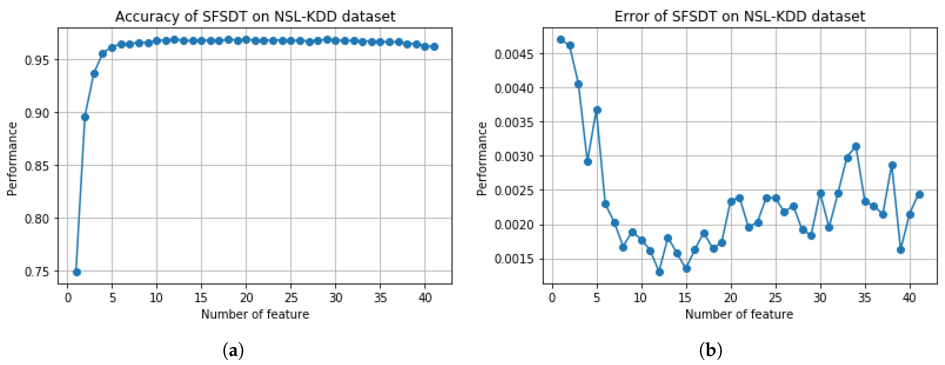
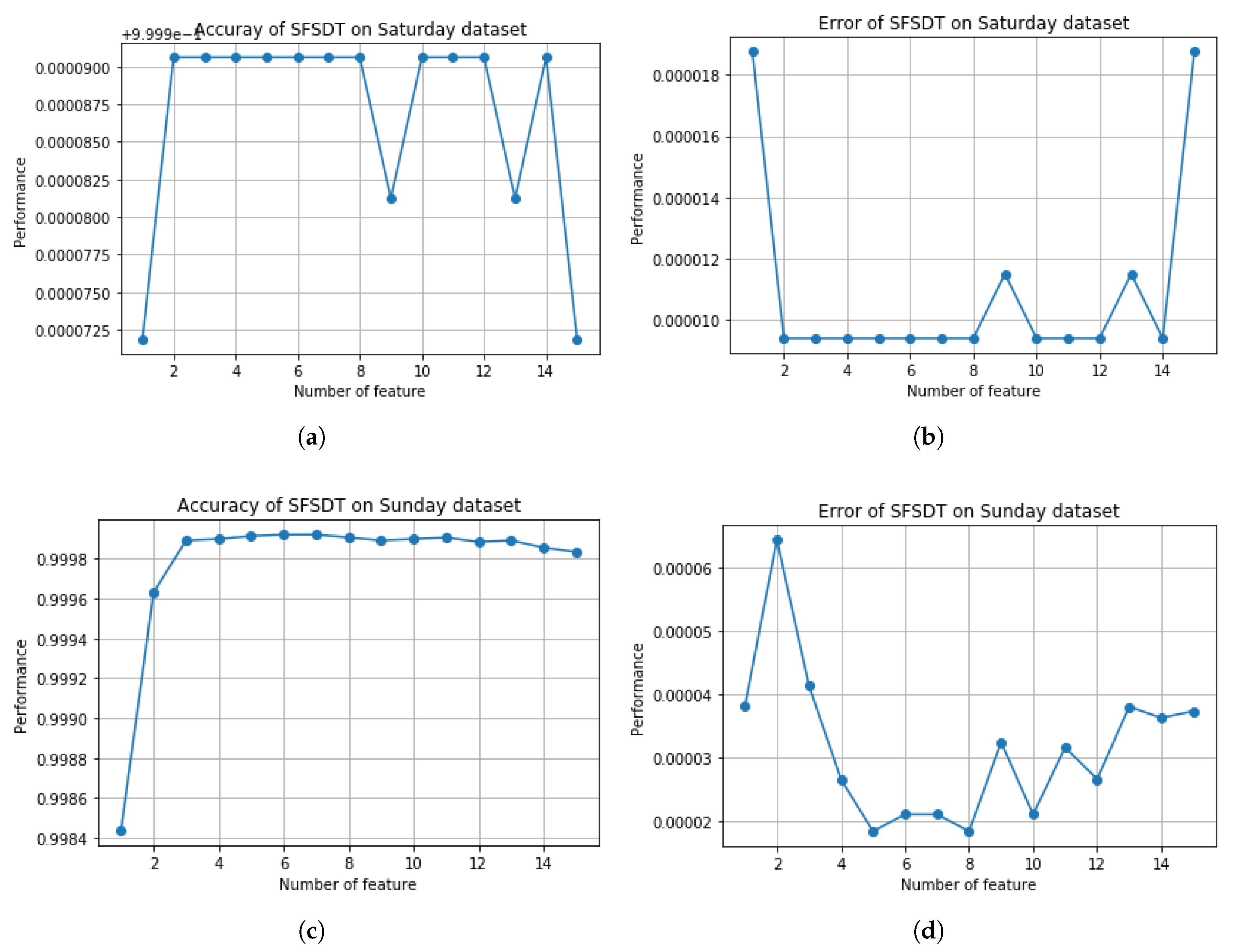
The proposed SFSDT model is implemented on both datasets including NSL-KDD and ISCX. The original feature number of these datasets are 41 and 15, respectively. This model visualizes how much accuracy and error scores obtained for each combination number of features in each dataset.
In NSL-KDD dataset, the results of SFSDT model are plotted in Figure 9a,b. From observation, the proposed model achieved the highest accuracy 0.969017 at the number of combination features is k = 12 . Besides, the minimum error score at 12 combined features is 0.00336. Therefore, the best feature subset is selected including 12 features. The corresponding to the list of selected feature subset is [protocol_type, service, flag, src_bytes, logged_in, num_file_creations, is_guest_login, count, srv_count, dst_host_srv_diff_host_rate, dst_host_rerror_rate, dst_host_srv_rerror_rate].
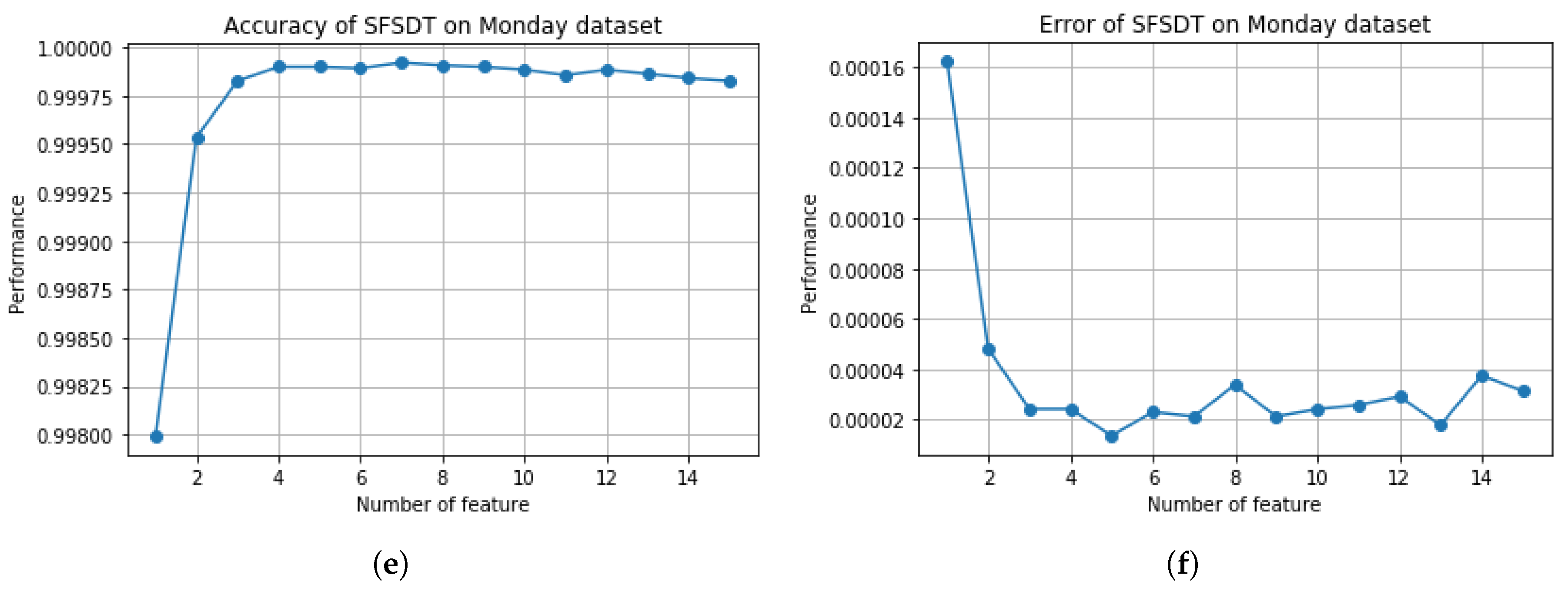
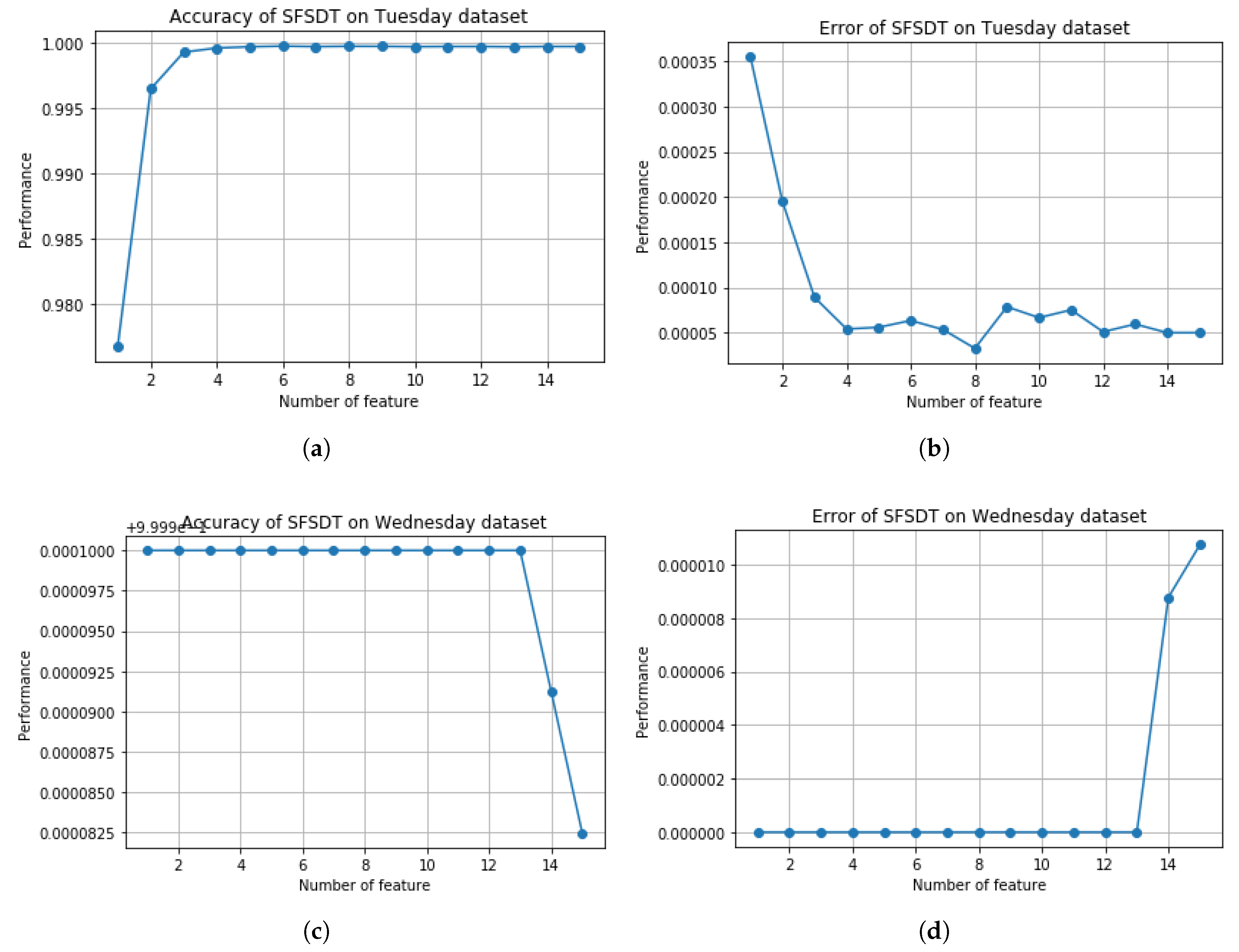
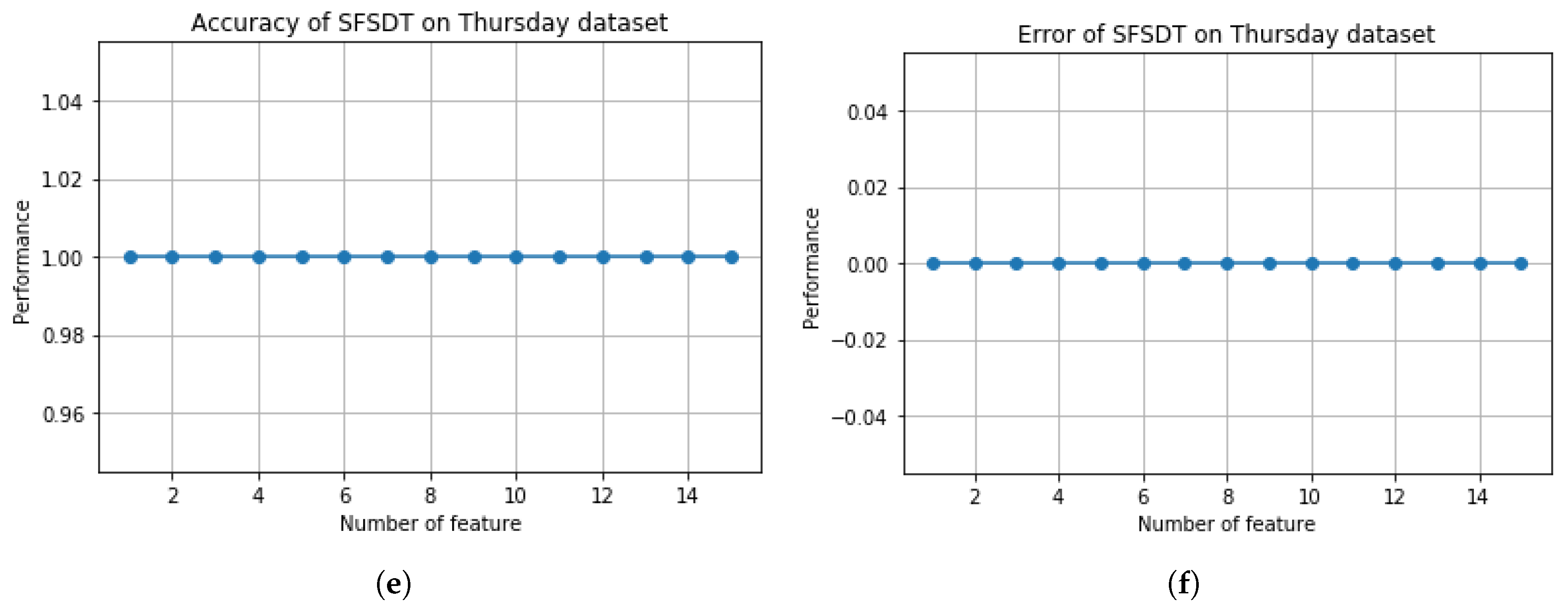
Similar to ISCX dataset, Figure 10 and Figure 11 show the accuracy and error scores of the proposed model for each day dataset. For example, the best feature subset obtained at 3 combined features which are [appName, totalDestinationBytes, source] in Saturday data.
In summary, the results of the selected feature subsets detail on two datasets are shown in Table 2. No.FF is the number of features in the original dataset. No.SF is the number of the best-selected feature subset by SFSDT algorithm.

4.2.2. Experiment 2

This experiment presents the results of variant RNN models are learned on the selected feature subset of experiment 1. These models are Simple RNN, LSTM, and GRU. The output class of ISCX dataset is [’Normal’, ’Attack’]. Hence, it is considered in binary classification in three learning models. [’Normal’] value is denoted by 0 and [’Attack’] value is denoted by 1. In NSL-KDD dataset, the output class includes non-attack and four types of attack, denoted by [’Normal’, ’R2L’, ’DoS’, ’U2R’, ’Probe’]. In experiment, visualization of ROC results of [’Normal’, ’R2L’, ’DoS’, ’U2R’, ’Probe’] are denoted by [’class 0’, ’ class 1’, ’class 2’, ’class 3’, ’class 4’], respectively. The number of output class is more than two, thus it is a multi-classification problem for three models. Therefore, confusion matrix and ROC measurement are used to visualize the attack type and non-attack detection results.
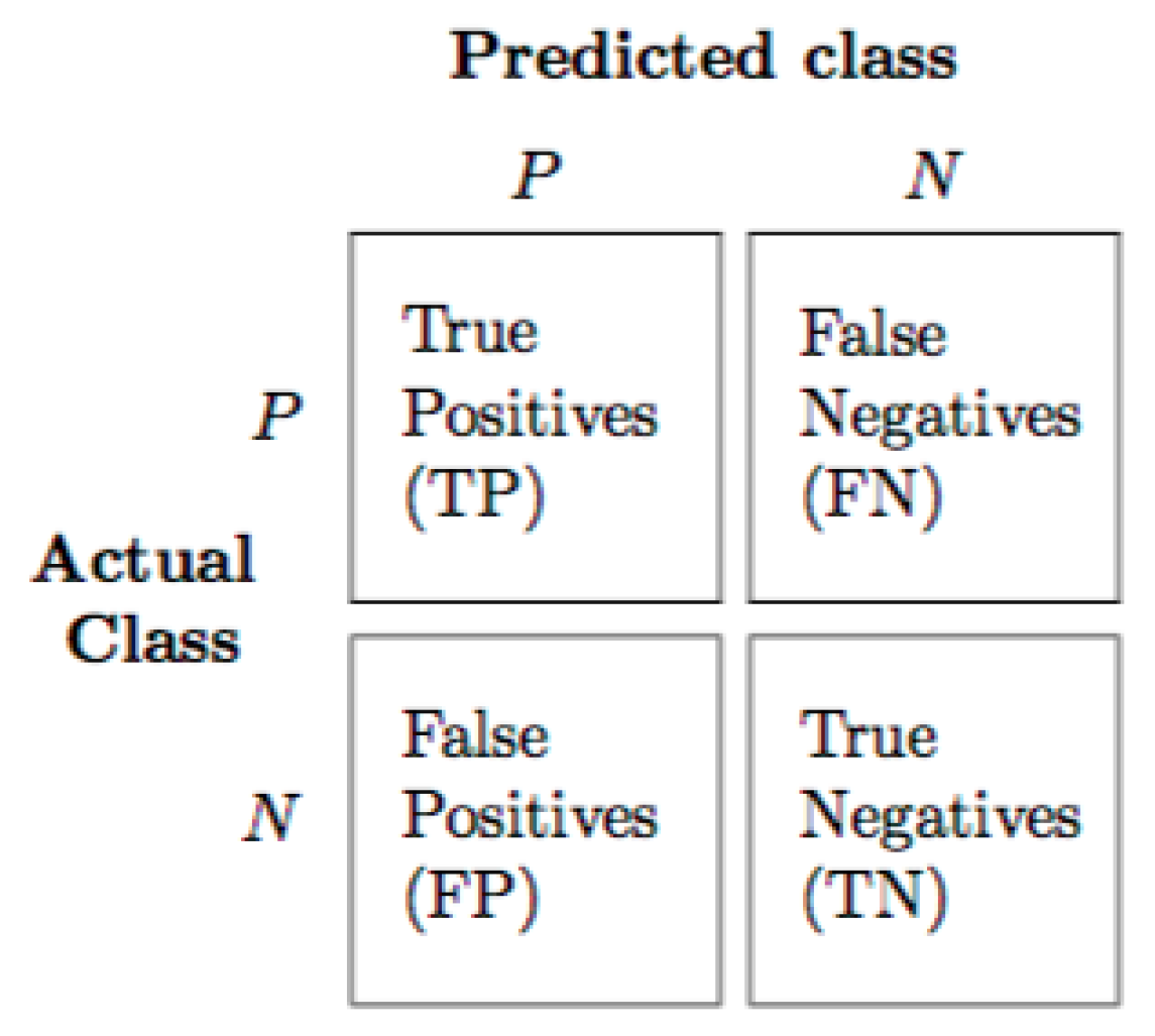
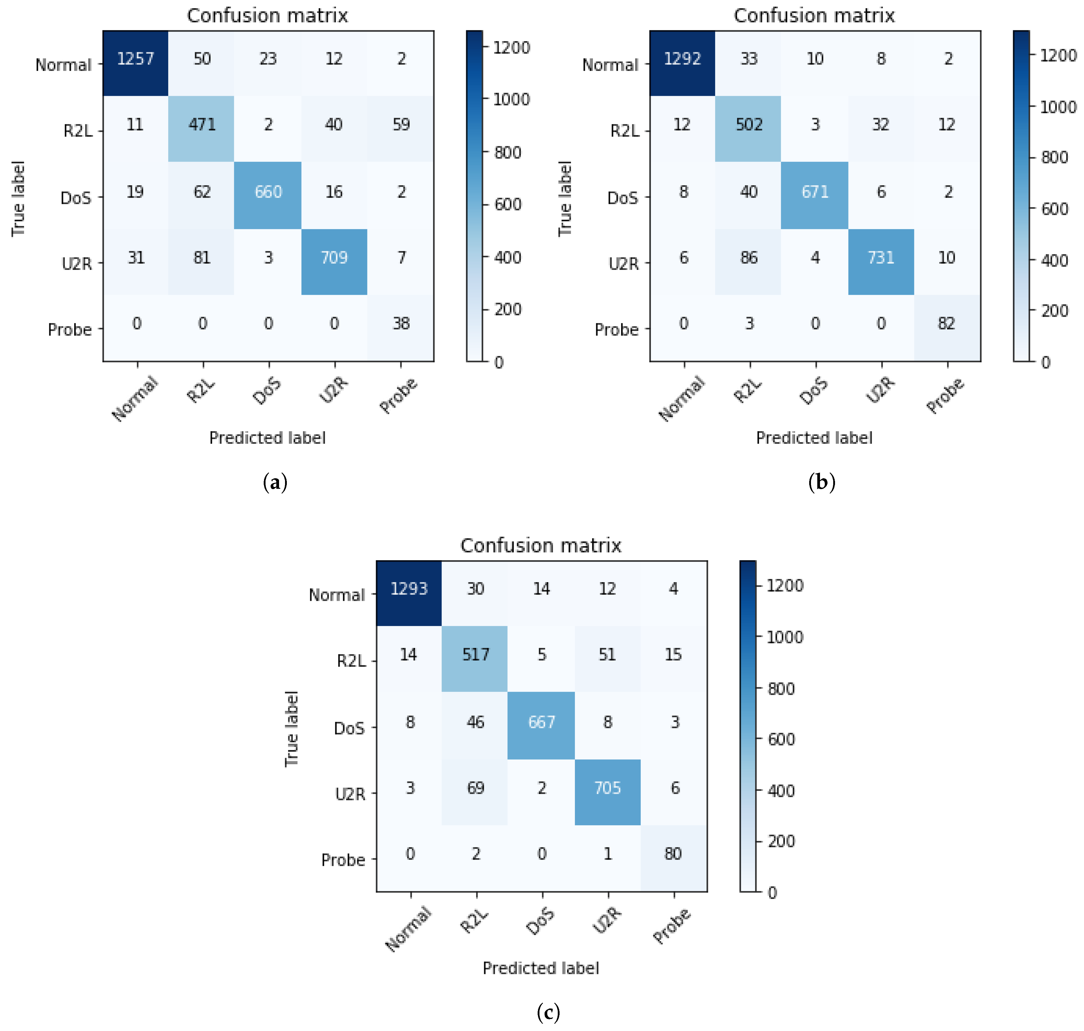
In the NSD-KDD dataset, the attack classification results are illustrated in Figure 12. The confusion matrix results display the number of correct and incorrect prediction compare to actual output class for each output class. The number of corrected predictions are displayed on the main diagonal of the confusion matrix.
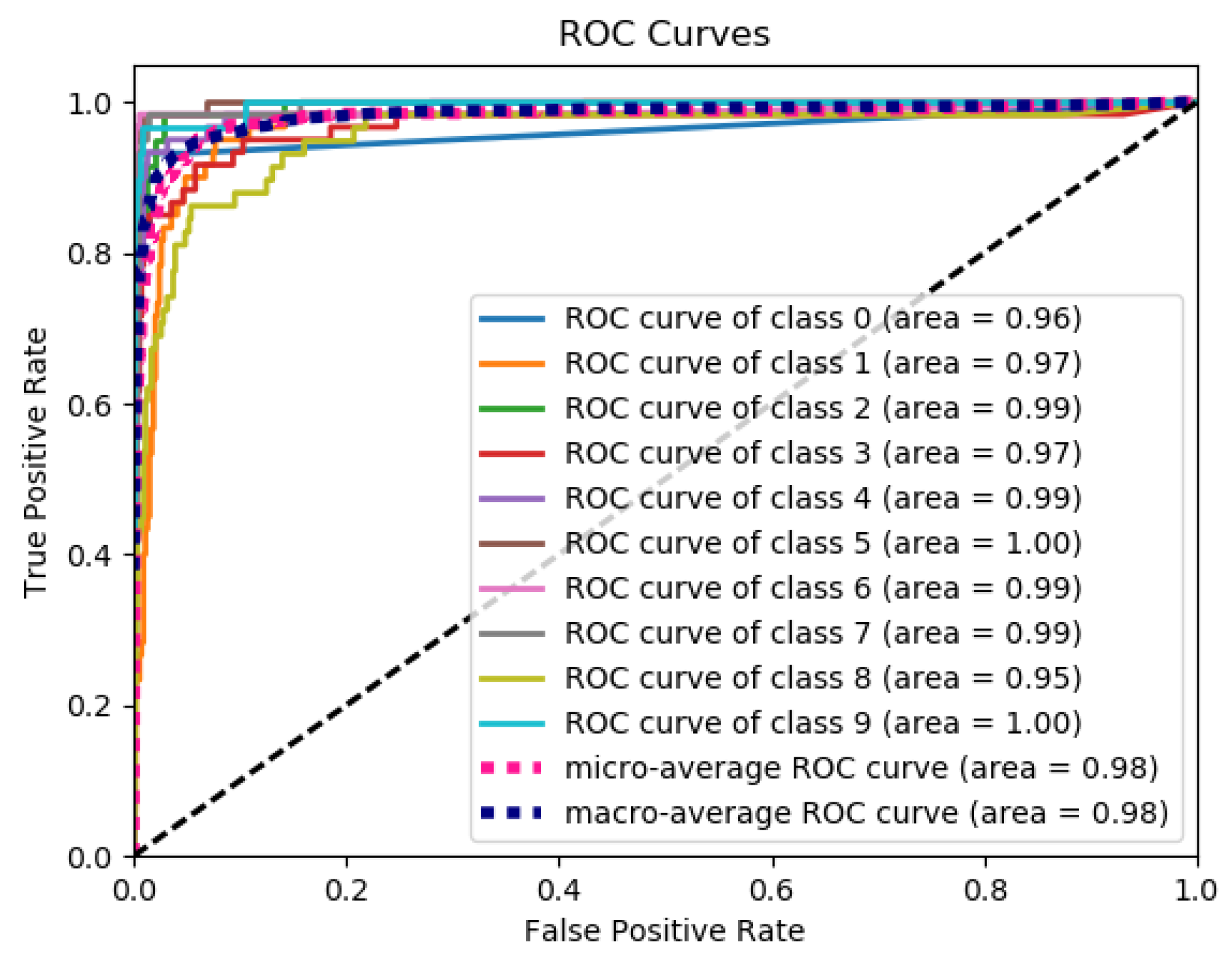
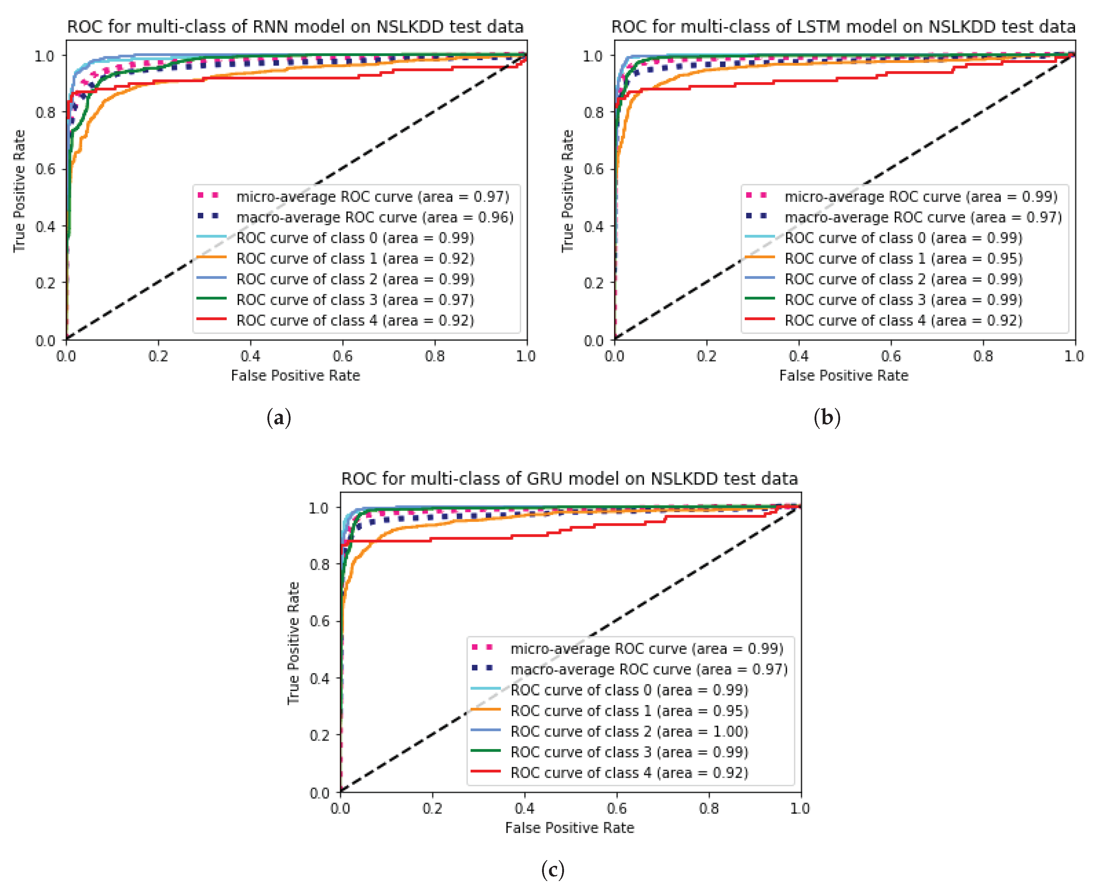
Besides, the ROC curve is used to measure the performance of different attacks detection on NSL-KDD dataset (see Figure 13). Most attack type detection achieved better results on LSTM and GRU models.
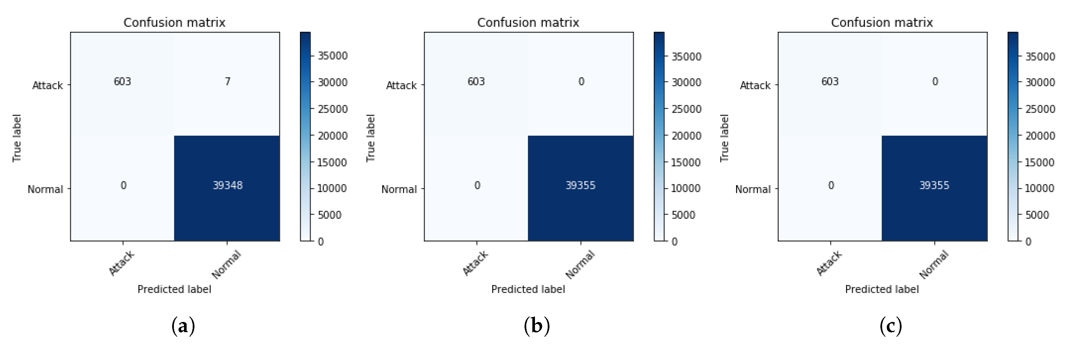
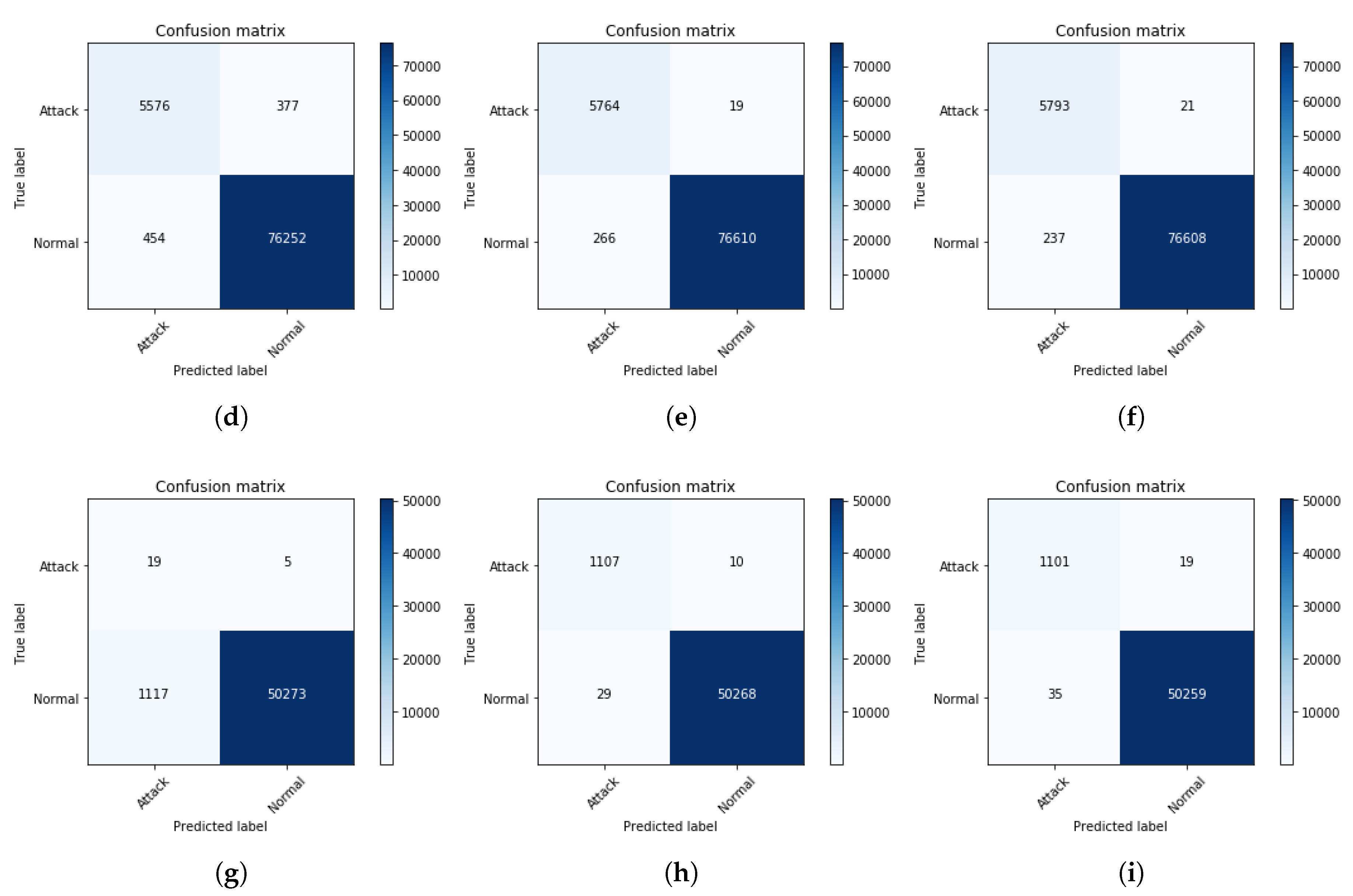
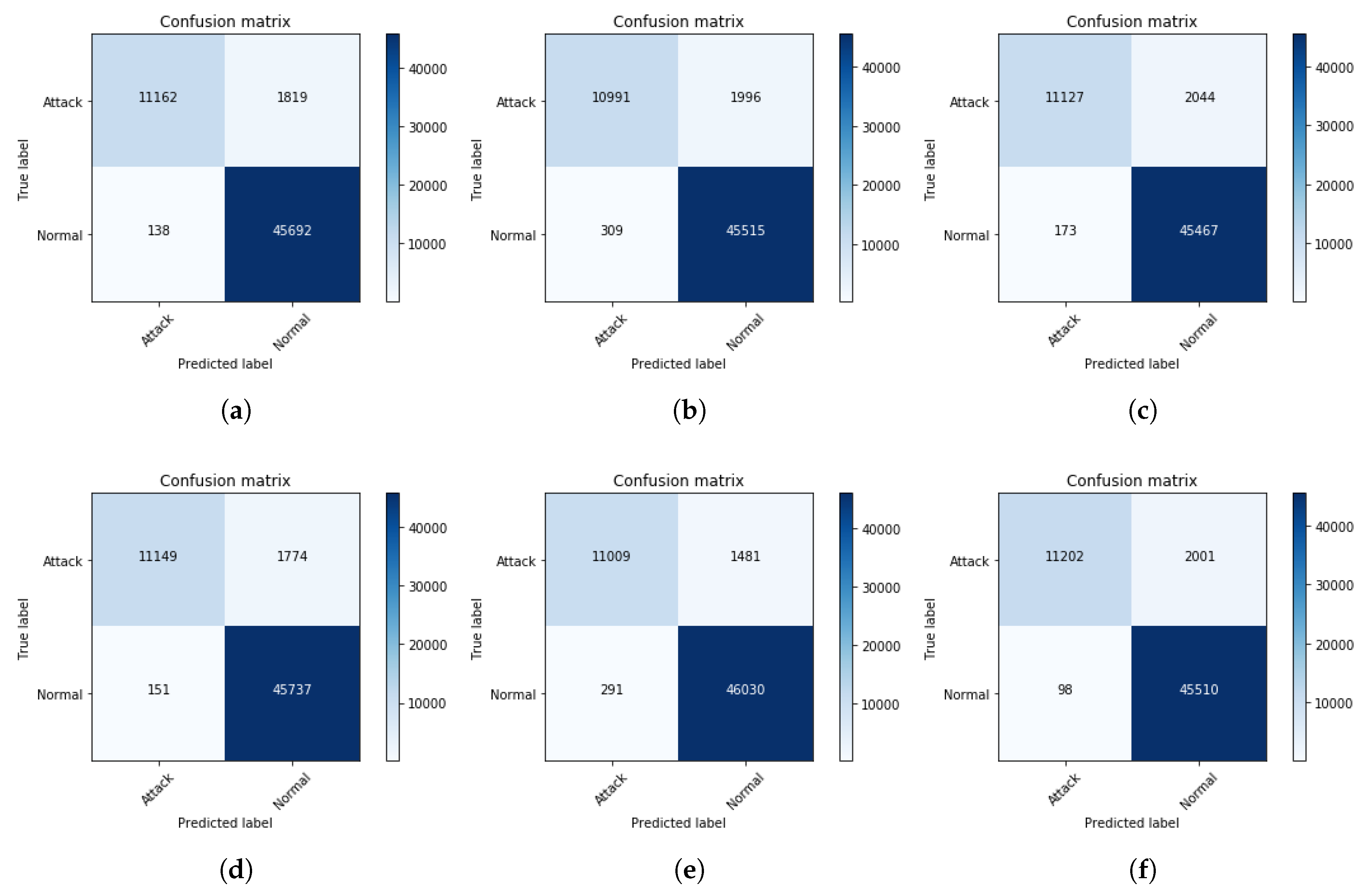
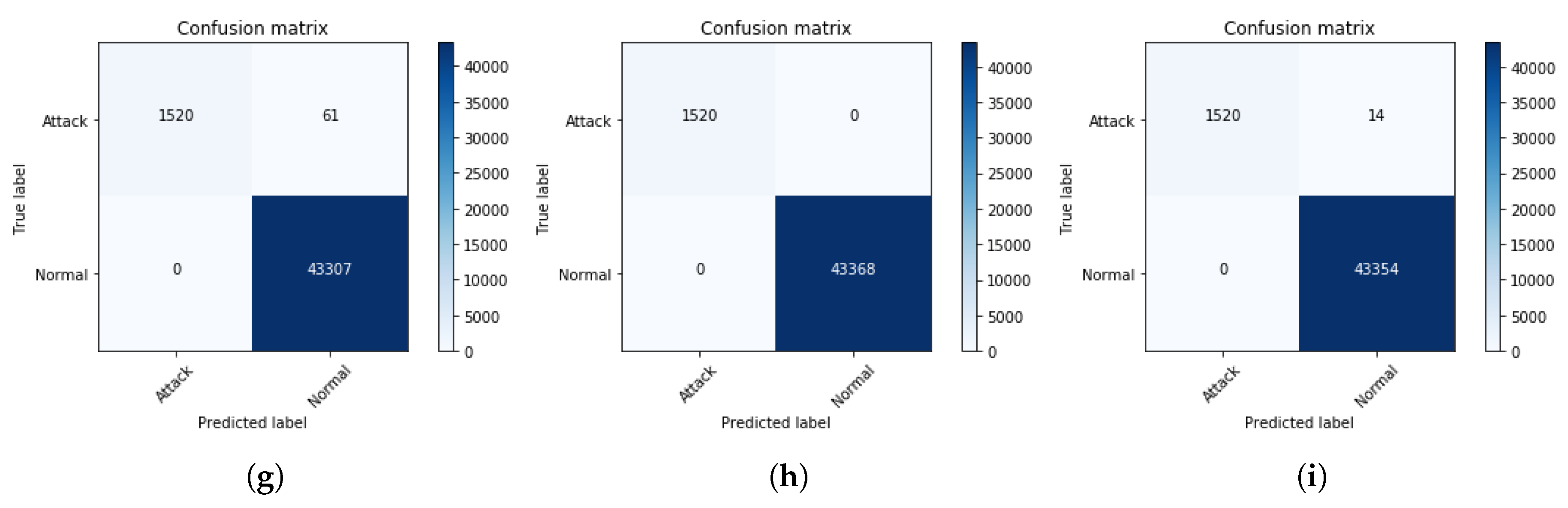
Similar to the ISCX dataset, the confusion matrix results of three models are displayed in Figure 14 (on Saturday, Sunday, and Monday data) and Figure 15 (on Tuesday, Wednesday, and Thursday data).
Based on the confusion matrix results, the accuracies of attack types detection in each dataset are calculated and summarized in Table 3. The average accuracies of RNN, LSTM, and GRU model on NSL-KDD subset feature data are 89.6%, 92%, and 91.8%. Similar to on ISCX subset feature data, 94.75%, 97.5%, and 97.08% are average obtained accuracies of RNN, LSTM, and GRU model, respectively. Therefore, the LSTM model has slightly better performance compared to the other models.

4.2.3. Experiment 3

As mentioned in 
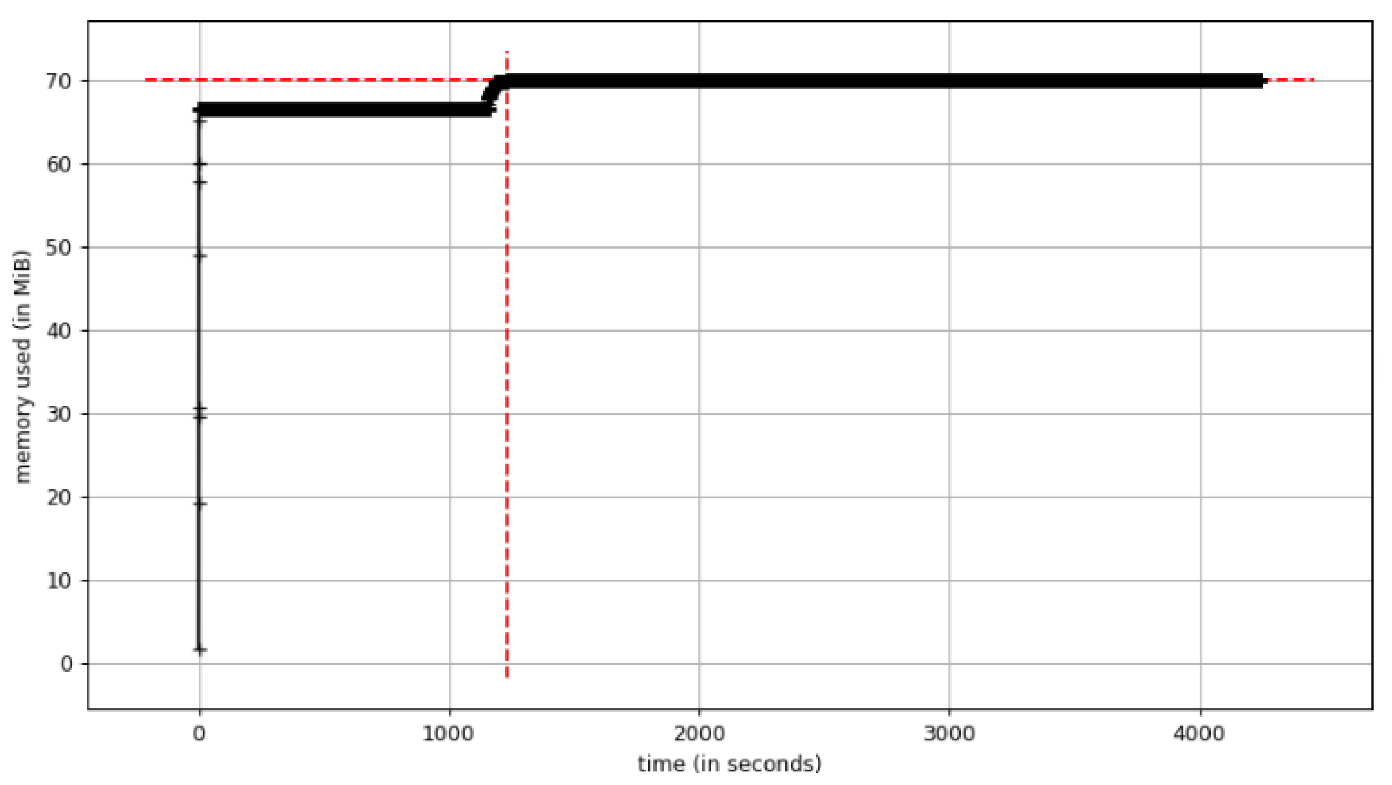
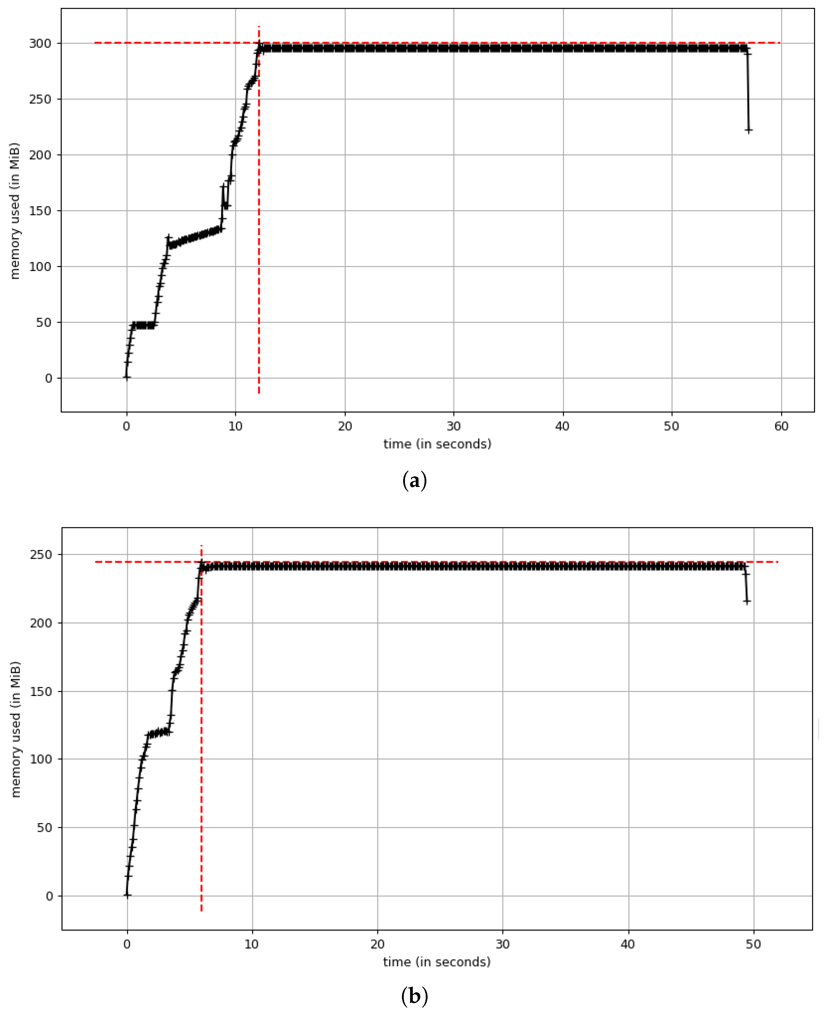
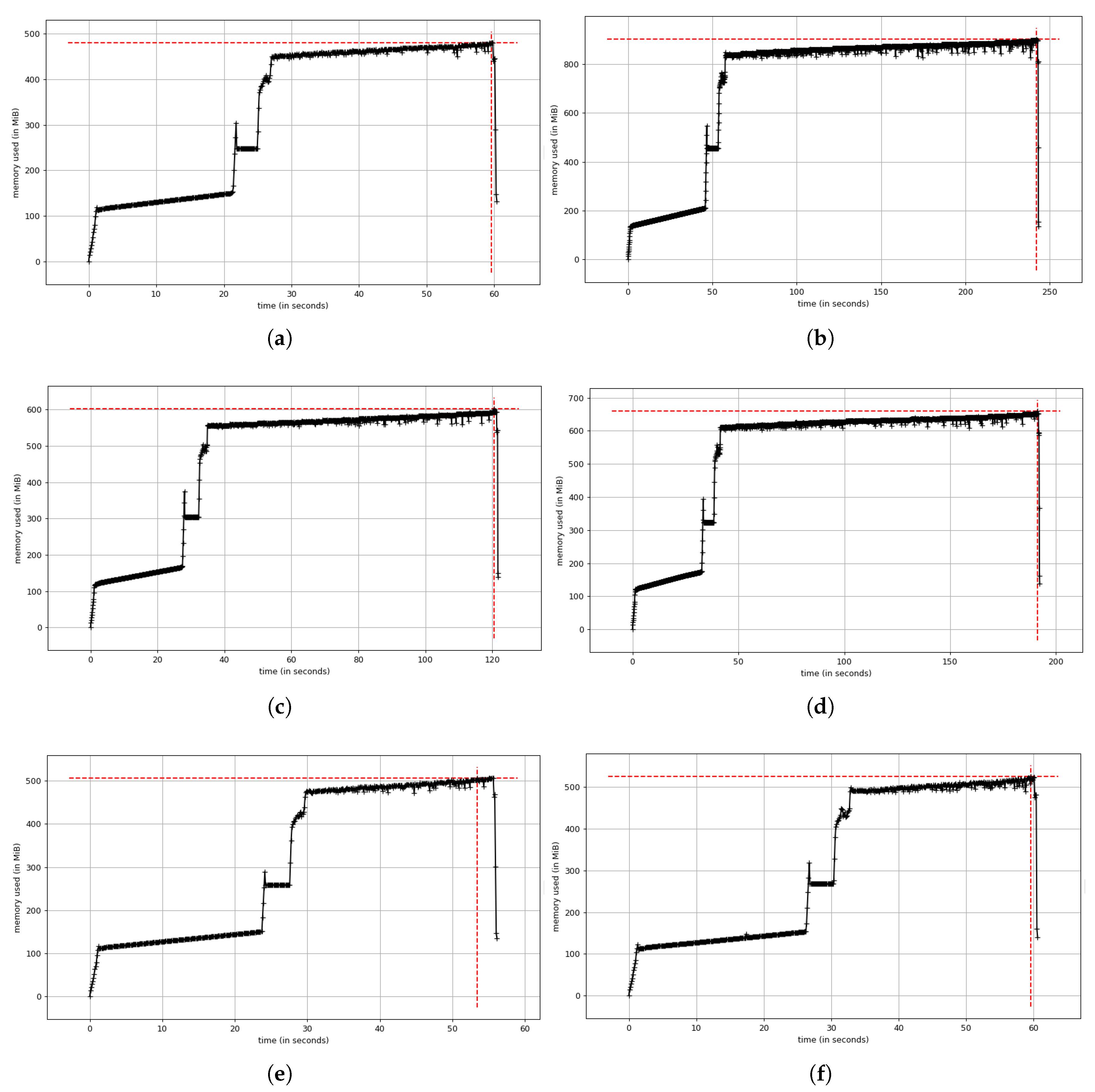
Section 4.2.2, the LSTM model obtained the best accuracy among three approach models. Hence, the LSTM model is selected to measure memory profiles in two cases. Case 1 calculates memory profiles on complete feature dataset of LSTM model. Case 2 calculates memory profiles on the best feature subset generated by SFSDT model of LSTM model. The memory profile reports to the memory used (in MiB unit) and time executed (in the second unit) of Python scripts. This experiment performed to measure running an executable of learning model, recording memory usage and plotting the recorded memory usage.
Figure 16 shows the memory profiles of LSTM model on NSL-KDD dataset. The used memory and the time for training of two cases are quite small different about memory profiles. In particular, memory used and time compiling of LSTM model is trained on selected feature subset occupied under 250 MiBs and near 50 s, respectively. While the LSTM model is trained on complete feature dataset obtained 300 MiBs and approximately 60 s corresponding to the memory used and time compiling. In the ISCX dataset, the memory profile results of LSTM model are plotted in
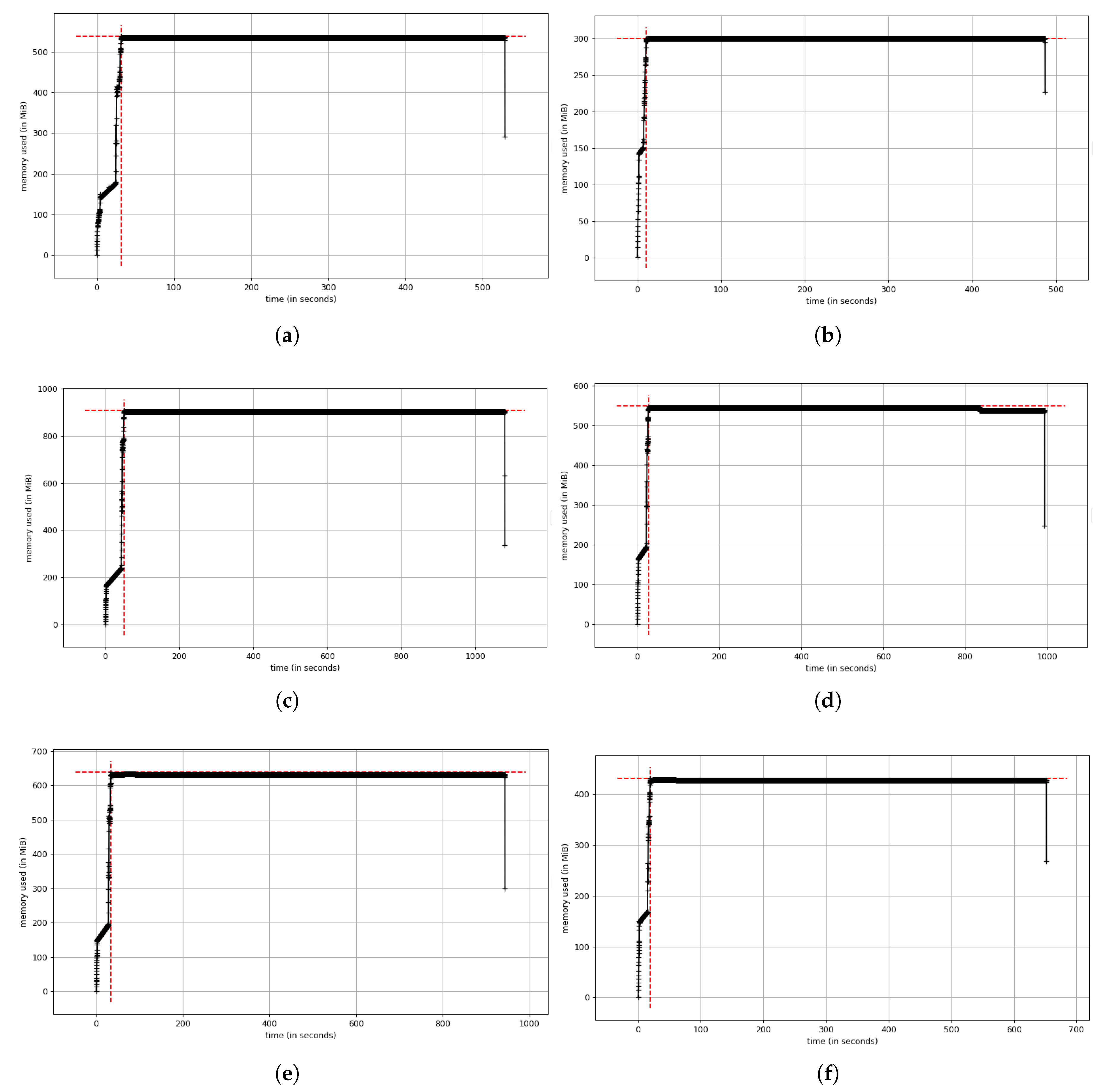
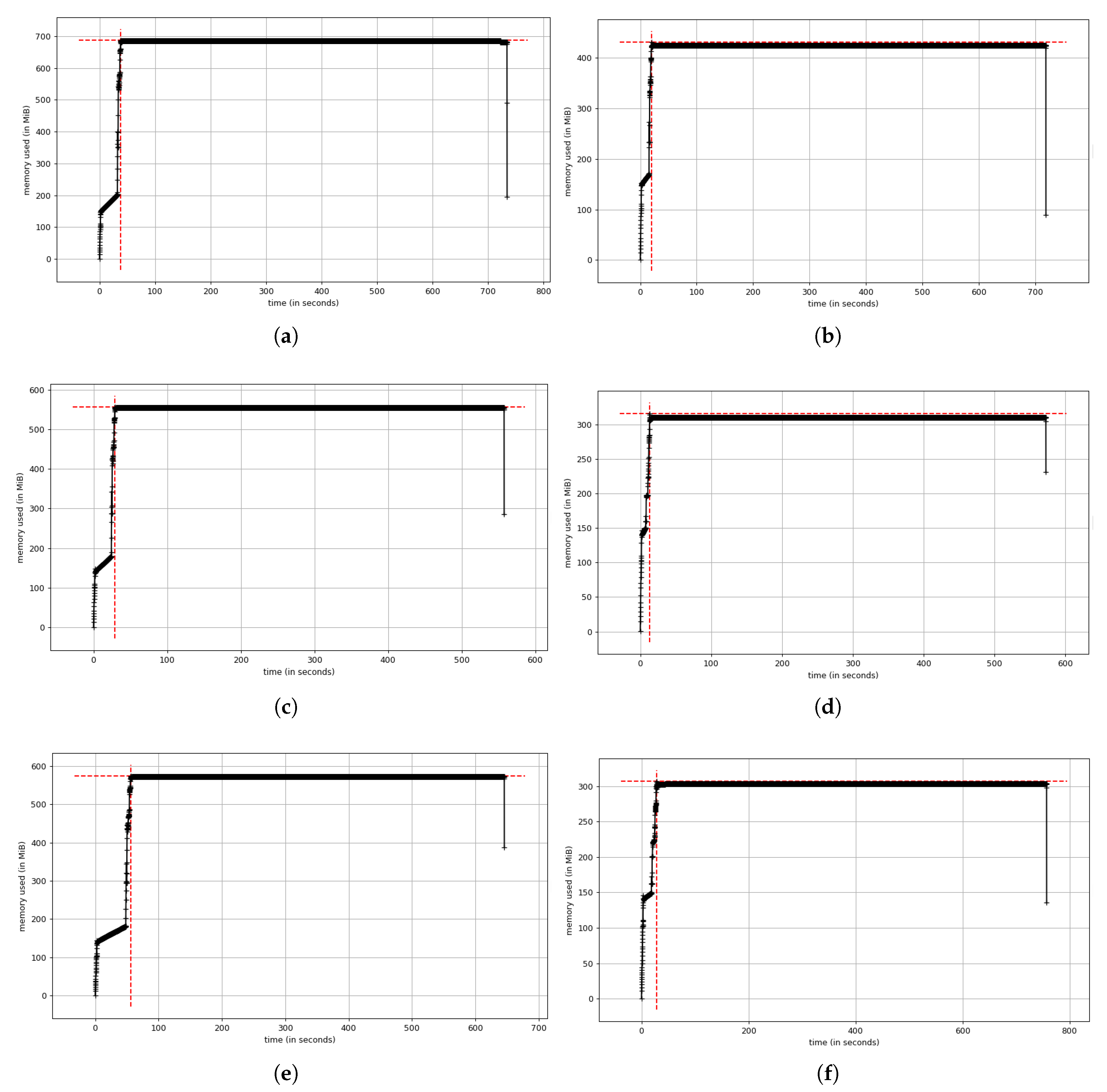
 Figure 17 and Figure 18.
In summary, the memory used and time executed of LSTM model on both cases ISCX dataset are listed in Table 4. Smaller values are better. Obviously, case 2 obtained almost better results of memory profiles on both memory used and time executed.
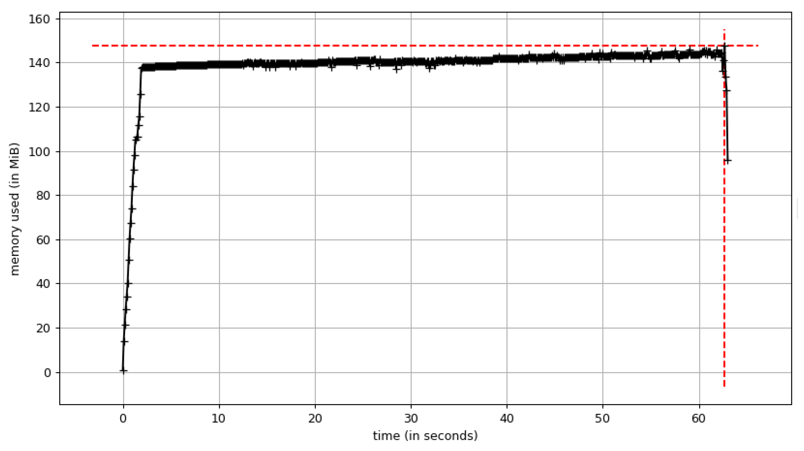
On the other hand, this work measured the memory profiler of the proposed SFSDT model to find the best feature subset on both datasets. Figure 19 shows the memory profiler of the proposed model on NSLKDD dataset. Besides, Figure 20 presents the memory profiler of the SFSDT model on ISCX dataset.
In summary, the memory profiler results of SFSDT model are pointed in Table 5. In NSL-KDD dataset, SFSDT model spent 63 s for time executed and used 145 MiB memory to generate and find the best features. Besides, in ISCX dataset, this proposed model spent averages 120.83 s and 573.33 MiB for time executed and memory used, respectively.

4.3. Discussion

Presently, there are many fields which contain big data, for example, finance, health care, stock, banking, etc. To analyze these datasets, it requires spending more effort with the different methods are used. It becomes a challenge with huge data with high dimensional features. A good feature selection technique helps us to analyze and evaluate to choose the important features in big data that ensure without losing important information. Besides, a good method helps reduce the effort for data analysis about time and cost. The proposed method can be applied to other fields which have big data to generate the best feature subset supporting further prediction model or using the result of the proposed method for other activities such as statistic, prediction, etc. In other words, this method is a low-cost design which helps data analyst can make a quick and accurate decision about what features are important and effect and then keeping them for supporting another further purpose.
In the proposed scheme, SFSDT’s goal is to generate and find the best feature subset from the complete feature set. The result of the proposed method on ISCX data are different in each day because their valuable data are different, even though each day the dataset has the same 15 original features. Hence, the obtained result of the proposed depends on the values of features. Therefore, when there is suspicious traffic with the different feature sets, the proposed model can accurately recognize it, to generate feature subsets which contain this different feature and then evaluate these subsets are the best feature or not. Besides, the proposed SFSDT goal is a feature selection based on the learning model. This proposed model can solve the high-dimensional data leading to the curse of dimensionality phenomenon in big data. The results of experiment 3 show that the proposed method can find the best feature subset in short time and small memory used.
Furthermore, the variant RNNs applied to the best feature subset can reduce the amount of required computation as well as improve performance accuracies on each attack classification and the average accuracy of classification IDS model. In particular, this work compares the proposed model to previous models on two criteria including detection of attack types and intrusion detection accuracies on both IDS datasets.
First, Table 6 and Table 7 show the comparison accuracies of detecting attack types between the proposed models to in advance IDS models on NSL-KDD dataset and ISCX dataset, respectively. Based on the results obtained, LSTM and GRU models outperform than others. In particular, the accurate detection of U2R and R2L attacks are improved significantly on LSTM and GRU models.
Second, Table 8 and Table 9 show the comparison results of the approached models to well-known IDS models on both datasets. The approached LSTM model outperformed accuracies than other IDS models on both datasets.

5. Conclusions

This paper proposed SFSDT is a feature selection model for improving various RNNs model in IDS field. Among three approached models, the LSTM model obtained the best accuracy performance on both IDS datasets. In particular, this paper addressed the existing problems in IDSs including improvement detection intrusion rate and type of each attack, especially, R2L and U2R. Besides, the experiment result illustrates the effects of the proposed feature selection model by reducing computation time and memory usage. The memory profile evaluation results show that the proposed algorithm not only reduced execution time and the amount of required memory but also significantly improved the performance of conventional LSTM model. Further, this proposed method is promising can be applied to process big data in other fields.

Author Contributions

Conceptualization, T.-T.-H.L.; Data curation, T.-T.-H.L. and Y.K.; Formal analysis, T.-T.-H.L. and Y.K.; Investigation, H.K.; Methodology, T.-T.-H.L.; Resources, H.K.; Software, T.-T.-H.L. and Y.K.; Supervision, H.K.; Validation, H.K.; Visualization, T.-T.-H.L. and Y.K.; Writing—original draft, T.-T.-H.L. and Y.K.; Writing—review & editing, H.K.

Funding

This work was supported by National IT Industry Promotion Agency(NIPA) grant funded by the Korea government(MSIT) (SS0249-19-1003, Development of Integrated Safety Management System for the Prevention of Industrial Accidents in Shipyard). This work is supported by Smart City R&D project of the Korea Agency for Infrastructure Technology Advancement(KAIA) grant funded by the Ministry of Land, Infrastructure and Transport(MOLIT), Ministry of Science and ICT(MSIT) (Grant 19NSPS-B149386-02).

Conflicts of Interest

The authors declare no conflict of interest.

Abbreviations

The following abbreviations are used in this manuscript:
IDSIntrusion Detection System
R2LRemote-to-Local
U2RUser-to-Root
SFSSequence Forward Selection
DTDecision Tree
RNNRecurrent Neural Network
LSTMLong Short-Term Memory
GRUGated Recurrent Unit
DoSDenial of Service
PCAPrinciple Component Analysis
DBMdeep Boltzmann machine
DBNdeep belief network
LDALinear Discriminant Analysis
CFcriterion function
KNNK Nearest Neighbour
SVMSupport Vector Machine
ROCReceive Operating Characteristic
TPTrue Positives
FNFalse Negatives
FPFalse Positives
TNTrue Negatives
TPRTrue Positive Rate
FPRFalse Positive Rate

References

  1. Chand, N.; Mishra, P.; Krishna, C.R.; Pilli, E.S.; Govil, M.C. A comparative analysis of SVM and its stacking with other classification algorithm for intrusion detection. In Proceedings of the 2016 International Conference on Advances in Computing, Communication & Automation (ICACCA) (Spring), Dehradun, India, 8–9 April 2016; pp. 1–6. [Google Scholar]
  2. Mukherjee, B.; Heberlein, L.T.; Levitt, K.N. Network intrusion detection. IEEE Netw. 1994, 8, 26–41. [Google Scholar] [CrossRef]
  3. Tsai, C.F.; Lin, C.Y. A triangle area based nearest neighbors approach to intrusion detection. Pattern Recognit. 2010, 43, 222–229. [Google Scholar] [CrossRef]
  4. Denning, D. An intrusion-detection model. J. Graph Theory 1987, SE-13, 222–232. [Google Scholar] [CrossRef]
  5. Masduki, B.W.; Ramli, K.; Saputra, F.A.; Sugiarto, D. Study on implementation of machine learning methods combination for improving attacks detection accuracy on Intrusion Detection System (IDS). In Proceedings of the 2015 International Conference on Quality in Research (QiR), Lombok, Indonesia, 10–13 August 2015; pp. 56–64. [Google Scholar]
  6. Kumar, G.; Kumar, K. Design of an evolutionary approach for intrusion detection. Sci. World J. 2013, 2013, 962185. [Google Scholar] [CrossRef]
  7. Tan, Z.; Jamdagni, A.; He, X.; Nanda, P.; Liu, R.P.; Hu, J. Detection of Denial-of-Service Attacks Based on Computer Vision Techniques. IEEE Trans. Comput. 2015, 64, 2519–2533. [Google Scholar] [CrossRef] [Green Version]
  8. Heidarian, Z.; Movahdinia, N.; Moghim, N.; Mahdinia, P. Intrusion Detection Based on Normal Traffic Specifications. Int. J. Comput. Netw. Inf. Secur. 2015, 9, 32–38. [Google Scholar] [CrossRef]
  9. Stavroulakis, P.; Stamp, M. Handbook of Information and Communication Security; Springer: New York, NY, USA, 2010. [Google Scholar]
  10. Liao, H.J.; Lin, C.H.R.; Lin, Y.C.; Tung, K.Y. Intrusion detection system: A comprehensive review. J. Netw. Comput. Appl. 2013, 36, 16–22. [Google Scholar] [CrossRef]
  11. Mar, J.; Hsiao, I.F.; Yeh, Y.C.; Kuo, C.C.; Wu, S.R. Intelligent intrusion detection and robust null defense for wireless networks. Int. J. Innov. Comput. Inf. Control 2012, 8, 3341–3359. [Google Scholar]
  12. Sabahi, F.; Movaghar, A. Intrusion detection: A survey. In Proceedings of the 2008 Third International Conference on Systems and Networks Communications, Sliema, Malta, 26–31 October 2008; pp. 23–26. [Google Scholar]
  13. Li, L.; Zhang, G.; Nie, J.; Niu, Y.; Yao, A. The application of genetic algorithm to intrusion detection in MP2P network. In Proceedings of the Third International Conference on Advances in Swarm Intelligence, Shenzhen, China, 17–20 June 2012; pp. 390–397. [Google Scholar]
  14. Kartit, A.; Saidi, A.; Bezzazi, F.; Marraki, M.E.; Radi, A. A new approach to intrusion detection system. J. Theor. Appl. Inf. Technol. 2012, 36, 284–289. [Google Scholar]
  15. Lazarevic, A.; Kumar, V.; Srivastava, J. Managing Cyber Threats: Issues, Approaches, and Challenges; Springer: New York, NY, USA, 2005. [Google Scholar]
  16. Murali, A.; Rao, M. A survey on intrusion detection approaches. In Proceedings of the First International Conference Information and Communication Technologies, Karachi, Pakistan, 27–28 August 2005; pp. 233–240. [Google Scholar]
  17. Modi, C.; Patel, D.; Borisaniya, B.; Patel, H.; Patel, A.; Rajarajan, M. A survey of intrusion detection techniques in Cloud. J. Netw. Comput. Appl. 2013, 36, 42–57. [Google Scholar] [CrossRef]
  18. Xie, M.; Han, S.; Tian, B.; Parvin, S. Anomaly detection in wireless sensor networks: A survey. J. Netw. Comput. Appl. 2011, 34, 1302–1325. [Google Scholar] [CrossRef]
  19. Kolias, C.; Kambourakis, G.; Maragoudakis, M. Swarm intelligence in intrusion detection: A survey. Comput. Secur. 2011, 30, 625–642. [Google Scholar] [CrossRef]
  20. Garcia-Teodoro, P.; Diaz-Verdejo, J.; Macia-Fernandez, G.; Vazquez, E. Anomaly-based network intrusion detection: Techniques, systems and challenges. Comput. Secur. 2009, 28, 18–28. [Google Scholar] [CrossRef]
  21. Alomari, O.; Othman, Z.A. Bees algorithm for feature selection in network anomaly detection. J. Appl. Sci. Res. 2012, 8, 1748–1756. [Google Scholar]
  22. Abolhasanzadeh, B. Nonlinear dimensionality reduction for intrusion detection using auto encoder bottleneck features. In Proceedings of the 2015 7th Conference on Information and Knowledge Technology (IKT), Urmia, Iran, 26–28 May 2015; pp. 1–5. [Google Scholar]
  23. Fiore, U.; Palmieri, F.; Castiglione, A.; de Santis, A. Network anomaly detection with the restricted Boltzmann machine. Neurocomputing 2013, 122, 13–23. [Google Scholar] [CrossRef]
  24. Alom, M.Z.; Bontupalli, V.; Taha, T.M. Intrusion detection using deep belief networks. In Proceedings of the National Aerospace and Electronics Conference (NAECON), Dayton, OH, USA, 15–19 June 2015; pp. 339–344. [Google Scholar]
  25. Anyanwu, L.O.; Keengwe, J.; Arome, G.A. Scalable Intrusion Detection with Recurrent Neural Networks. In Proceedings of the IEEE 2010 Seventh International Conference on Information Technology: New Generations, Las Vegas, NV, USA, 12–14 April 2010; pp. 919–923. [Google Scholar]
  26. Kim, J.; Kim, J.; Thu, H.L.T.; Kim, H. Long Short Term Memory Recurrent Neural Network Classifier for Intrusion Detection. In Proceedings of the 2016 International Conference on Platform Technology and Service (PlatCon), Jeju, Korea, 15–17 February 2016; pp. 1–5. [Google Scholar]
  27. Le, T.T.H.; Kim, J.; Kim, H. An Effective Intrusion Detection Classifier Using Long Short-Term Memory with Gradient Descent Optimization. In Proceedings of the International Conference on Platform Technology and Service (PlatCon), Busan, Korea, 13–15 February 2017; pp. 1–5. [Google Scholar]
  28. Hodo, E.; Bellekens, X.; Hamilton, A.; Tachtatzis, C.; Atkinson, R. Shallow and Deep Networks Intrusion Detection System: A Taxonomy and Survey. arXiv, 2017; arXiv:1701.02145. [Google Scholar]
  29. Ferri, F.; Pudil, P.; Hatef, M.; Kittler, J. Comparative Study of Techniques for Large Scale Feature Selection. Mach. Intell. Pattern Recognit. 1994, 16, 403–413. [Google Scholar]
  30. Quinlan, J.R. Induction of decision trees. Mach. Learn. 1986, 1, 81–106. [Google Scholar] [CrossRef] [Green Version]
  31. Jaeger, H. A Tutorial on Training Recurrent Neural Networks, Covering BPPT, RTRL, EKF and the Echo State Network Approach; GMD-Forschungszentrum Informationstechnik: Berlin, Germany, 2002. [Google Scholar]
  32. Pascanu, R.; TMikolov, T.; Bengio, Y. On the difficulty of training recurrent neural networks. In Proceedings of the 30th International Conference on International Conference on Machine Learning, Atlanta, GA, USA, 16–21 June 2013; pp. 1310–1318. [Google Scholar]
  33. Hochreiter, S.; Schmidhuber, J. Long short-term memory. Neural Comput. 1997, 9, 1735–1780. [Google Scholar] [CrossRef] [PubMed]
  34. Cho, K.; van Merrienboer, B.; Bahdanau, D.; Bengio, Y. On the properties of neural machine translation: Encoder-decoder approaches. arXiv, 2014; arXiv:1409.1259. [Google Scholar]
  35. Tavallaee, M.; Bagheri, E.; Lu, W.; Ghorbani, A. A detailed analysis of the kdd cup 99 data set. In Proceedings of the 2009 IEEE Symposium on Computational Intelligence for Security and Defense Applications (CISDA), Ottawa, ON, Canada, 8–10 July 2009. [Google Scholar]
  36. Shiravi, A.; Shiravi, H.; Tavallaee, M.; Ghorbani, A.A. Toward developing a systematic approach to generate benchmark datasets for intrusion detection. Comput. Secur. 2012, 31, 357–374. [Google Scholar] [CrossRef]
  37. Ingre, B.; Yadav, A. Performance Analysis of NSL-KDD dataset using ANN. In Proceedings of the International Conference Signal Processing and Communication Engineering Systems (SPACES), Guntur, India, 2–3 January 2015; pp. 92–96. [Google Scholar]
  38. Revathi, S.; Malathi, A. A Detailed Analysis on NSL-KDD Dataset Using Various Machine Learning Techniques for Intrusion Detection. IJERT 2013, 2, 1848–1853. [Google Scholar]
  39. Yang, Y.; Zheng, K.; Wu, C.; Niu, X.; Yang, Y. Building an Effective Intrusion Detection System Using the Modified Density Peak Clustering Algorithm and Deep Belief Networks. Appl. Sci. 2019, 9, 238. [Google Scholar] [CrossRef]
  40. Mzila, P.; Eric Dube, E. The effect of destination linked feature selection in real-time network intrusion detection. In Proceedings of the 8th International Conference on Internet Monitoring and Protection, Rome, Italy, 23–28 June 2013; pp. 8–13. [Google Scholar]
  41. Ma, T.; Wang, F.; Cheng, J.; Yu, Y.; Chen, X. A Hybrid Spectral Clustering and Deep Neural Network Ensemble Algorithm for Intrusion Detection in Sensor Networks. Sensors 2016, 16, 1701. [Google Scholar] [CrossRef]
  42. Javaid, A.; Niyaz, Q.; Sun, W.; Alam, M. A deep learning approach for network intrusion detection system. In Proceedings of the 9th EAI International Conference on Bio-Inspired Information and Communications Technologies (Formerly BIONETICS), New York, NY, USA, 2–5 December 2016; pp. 21–26. [Google Scholar]
  43. Tang, T.A.; Mhamdi, L.; McLernon, D.; Zaidi, S.A.R.; Ghogho, M. Deep learning approach for network intrusion detection in software defined networking. In Proceedings of the 2016 International Conference on Wireless Networks and Mobile Communications (WINCOM), Fez, Morocco, 26–29 October 2016; pp. 258–263. [Google Scholar]
  44. Imamverdiyev, Y.; Abdullayeva, F. Deep Learning Method for Denial of Service Attack Detection Based on Restricted Boltzmann Machine. Big Data 2018, 6, 159–169. [Google Scholar] [CrossRef] [PubMed]
  45. Meira, J. Comparative Results with Unsupervised Techniques in Cyber Attack Novelty Detection. Proceedings 2018, 2, 1191. [Google Scholar] [CrossRef]
  46. Yin, C.; Zhu, Y.; Fei, J.; He, X. A deep learning approach for intrusion detection using recurrent neural networks. IEEE Access 2017, 5, 21954–21961. [Google Scholar] [CrossRef]
Figure 1. The proposed IDS framework.
Applsci 09 01392 g001
Figure 2. The feature selection concept.
Applsci 09 01392 g002
Figure 3. RNN architecture by time.
Applsci 09 01392 g003
Figure 4. An architecture of long short-term memory networks by time.
Applsci 09 01392 g004
Figure 5. An architecture of Gated Recurrent Unit networks by time.
Applsci 09 01392 g005
Figure 6. Confusion matrix.
Applsci 09 01392 g006
Figure 7. ROC curve example for multi-classes.
Applsci 09 01392 g007
Figure 8. Memory profiler example.
Applsci 09 01392 g008
Figure 9. Visualization performance of SFSDT model on NSL-KDD dataset. (a) accuracy score & (b) error score.
Applsci 09 01392 g009
Figure 10. Visualization accuracy and error scores of SFSDT model on each day of ISCX dataset. (a) & (b) Saturday data; (c) & (d) Sunday data; (e) & (f) Monday data.
Applsci 09 01392 g010aApplsci 09 01392 g010b
Figure 11. Visualization accuracy and error scores of SFSDT model on each day of ISCX dataset. (a) & (b) Tuesday data; (c) & (d) Wednesday data; (e) & (f) Thursday data.
Applsci 09 01392 g011aApplsci 09 01392 g011b
Figure 12. Confusion matrix of three IDS models on NSL-KDD dataset. (a) Simple RNN model (b) LSTM model (c) GRU model.
Applsci 09 01392 g012
Figure 13. ROC for multi-class of three IDS models on NSL-KDD dataset. (a) RNN model (b) LSTM model (c) GRU model.
Applsci 09 01392 g013
Figure 14. Confusion matrix results of three approach models RNN, LSTM, and GRU on ISCX selected feature subset. (ac) on Saturday, (df) on Sunday, (gi) on Monday.
Applsci 09 01392 g014aApplsci 09 01392 g014b
Figure 15. Confusion matrix results of three approach models RNN, LSTM, and GRU on ISCX selected feature subset. (ac) on Tuesday, (df) on Wednesday, (gi) on Thursday.
Applsci 09 01392 g015aApplsci 09 01392 g015b
Figure 16. Memory profile of two models on NSL-KDD dataset. (a) Original feature dataset; (b) Selected feature subset.
Applsci 09 01392 g016
Figure 17. Memory profile results of LSTM model on complete feature data and selected feature subset data respectively. (a) & (b) Saturday data; (c) & (d) Sunday data; (e) & (f) Monday data.
Applsci 09 01392 g017
Figure 18. Memory profile results of LSTM model on complete feature data and selected feature subset data respectively. (a) & (b) Tuesday data; (c) & (d) Wednesday data; (e) & (f) Thursday data.
Applsci 09 01392 g018
Figure 19. Memory profile results of SFSDT model to select the best feature subset on NSLKDD dataset.
Applsci 09 01392 g019
Figure 20. Memory profile results of SFSDT model to select the best feature subset on ISCX dataset. (a) Saturday data; (b) Sunday data; (c) Monday data; (d) Tuesday data; (e) Wednesday data; (f) Thursday data.
Applsci 09 01392 g020
Table 1. List of number of record for training and testing data.
DateTotal of RecordNo. TrainingNo. Testing
Saturday133,19493,23639,958
Sunday275,528192,87082,658
Monday171,380119,96651,414
Tuesday192,041134,42957,612
Wednesday182,968128,07854,890
Thursday149,625104,73844,887
Table 2. The selected feature subset by SFSDT algorithm on two IDS datasets.
DatasetNo.FFNo.SFSelected Feature SubsetAccuracyError
protocol_type, service, flag, src_bytes,
logged_in, num_file_creations,
NSL-KDD4112is_guest_login, count, srv_count,0.9690170.00336
dst_host_srv_diff_host_rate,
dst_host_rerror_rate,
dst_host_srv_rerror_rate
Saturday data153appName, totalDestinationBytes, source0.9999910.00001
Sunday data157appName, direction, protocolName, sourcePort,0.9999200.00002
destination, destinationPort, startDateTime
Monday data157appName, totalDestinationBytes, direction, source,0.9999200.00002
destination, destinationPort, startDateTime
Tuesday data156totalSourceBytes, source, destination,0.9997190.00006
destinationPort, startDateTime, stopDateTime
Wednesday data153appName, totalSourceBytes, totalDestinationBytes10
Thursday data153appName, totalSourceBytes, source10
Table 3. The accuracy of attack types detection on two datasets.
DatasetAttackRNNLSTMGRU
Normal0.940.960.96
R2L0.810.890.86
NSL-KDDDoS0.880.920.91
U2R0.850.870.90
Probe1.000.960.96
Saturday dataNormal1.001.001.00
Attack0.991.001.00
Sunday dataNormal0.991.001.00
Attack0.941.000.99
Monday dataNormal0.981.001.00
Attack0.790.990.98
Tuesday dataNormal1.000.991.00
Attack0.860.850.84
Wednesday dataNormal1.000.991.00
Attack0.860.880.85
Thursday dataNormal1.001.001.00
Attack0.961.000.99
Table 4. The memory profiles of LSTM model on ISCX dataset.
DatasetMemory Used Case 1Memory Use Case 2Time Executed Case 1Time Executed Case 2
Saturday550300550480
Sunday90055011001000
Monday650450950650
Tuesday700450730710
Wednesday550310550570
Thursday580300650780
Table 5. The memory profiles of SFSDT model two IDS datasets.
DatasetMemory UsedTime Executed
NSL-KDD14563
Saturday48060
Sunday700240
Monday600120
Tuesday650190
Wednesday50055
Thursday51060
Table 6. Comparison accuracy detection of attack types on NSL-KDD dataset.
ModelNormal (%)DoS (%)Probe (%)U2R (%)R2L (%)
ANN [37]-77.776.610.534.6
J48 [38]87.588.386.075.588.9
CART [38]91.989.585.480.789.0
Naive Bayes [38]75.975.075.174.371.1
MDPCA-DBN [39]97.3881.0973.946.5017.25
RNN94881008581
LSTM9692968789
GRU9691969086
Table 7. Comparison accuracy detection of attack types results on ISCX dataset
ModelNormal (%)Attack (%)
NB [7]35.598.4
Bagged-NB [7]37.898.4
Boosted-NB [7]35.598.4
AMGA2-NB [7]95.292.7
TCM-KNN [40]97.2881.78
RNN99.590
LSTM96.6795.33
GRU10094.17
Table 8. Comparison accuracy detection results on NSL-KDD dataset
ModelAccuracy (%)
SCDNN [41]72.64
STL [42]74.38
DNN [43]75.75
Gaussian-Bernoulli RBM [44]73.23
Naive Bayes [38]74.28
J48 [38]80.6
ANN [37]81.2
CART [38]81.5
MDPCA-DBN [39]82.08
Zscore+Kmeans [45]90
RNN [46]81.29
RNN89.6
LSTM92
GRU91.8
Table 9. Comparison accuracy detection results on ISCX dataset
ModelAccuracy (%)
NB [7]43.2
Bagged-NB [7]45.3
Boosted-NB [7]43.2
AMGA2-NB [7]94.5
TCM-KNN [40]92.05
Zscore+Kmeans [45]95
RNN94.75
LSTM97.5
GRU97.08

