A Low-Complexity Resource Allocation Algorithm for Indoor Visible Light Communication Ultra-Dense Networks


Abstract
:1. Introduction
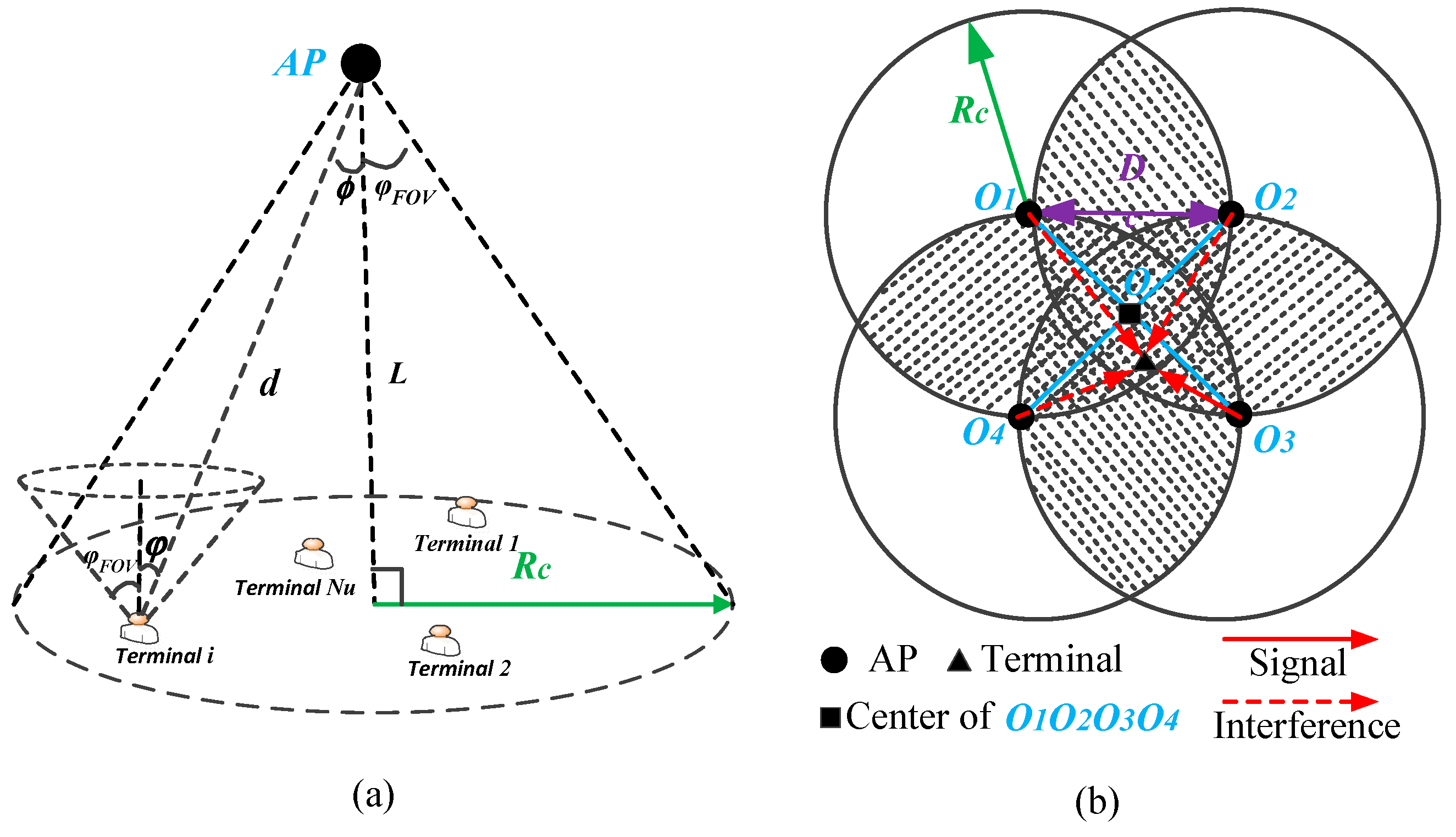
2. System Model
2.1. Channel Model
2.2. Network Model
3. Resource Allocation Algorithm
3.1. Convex Analysis of Resource Allocation Problem
3.2. The Proposed Multi-Cell Resource Allocation Algorithm
- If , the value of can be an arbitrary real number. Because , the value of can be an arbitrary real number. Combined with Equation (16.c), we have ;
- If , . Therefore, and the conclusion satisfies Equation (16c). According to the monotonic decreasing property of , we obtained that . Because , we have where is the inverse function of . By defining the notation , we have:
3.3. Algorithm Description and Asymptotic Complexity Analysis
| Algorithm 1. Low-Complexity Multi-Cell Resource Allocation Algorithm. |
| Input: the information of terminals and Aps |
| Output: the approximate optimal normalized resource ratio factor of each terminal |
| for calculate the break point for terminal i end for do the following steps for constitute the break point vector sort in descending order and obtain for calculate if break end end for calculate the approximate optimal normalized resource ratio factor end |
4. Simulation Results
4.1. Conditions
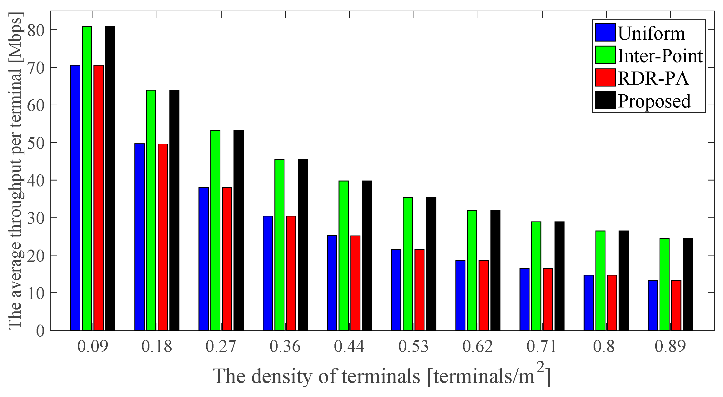
4.2. Analysis on Terminal Density
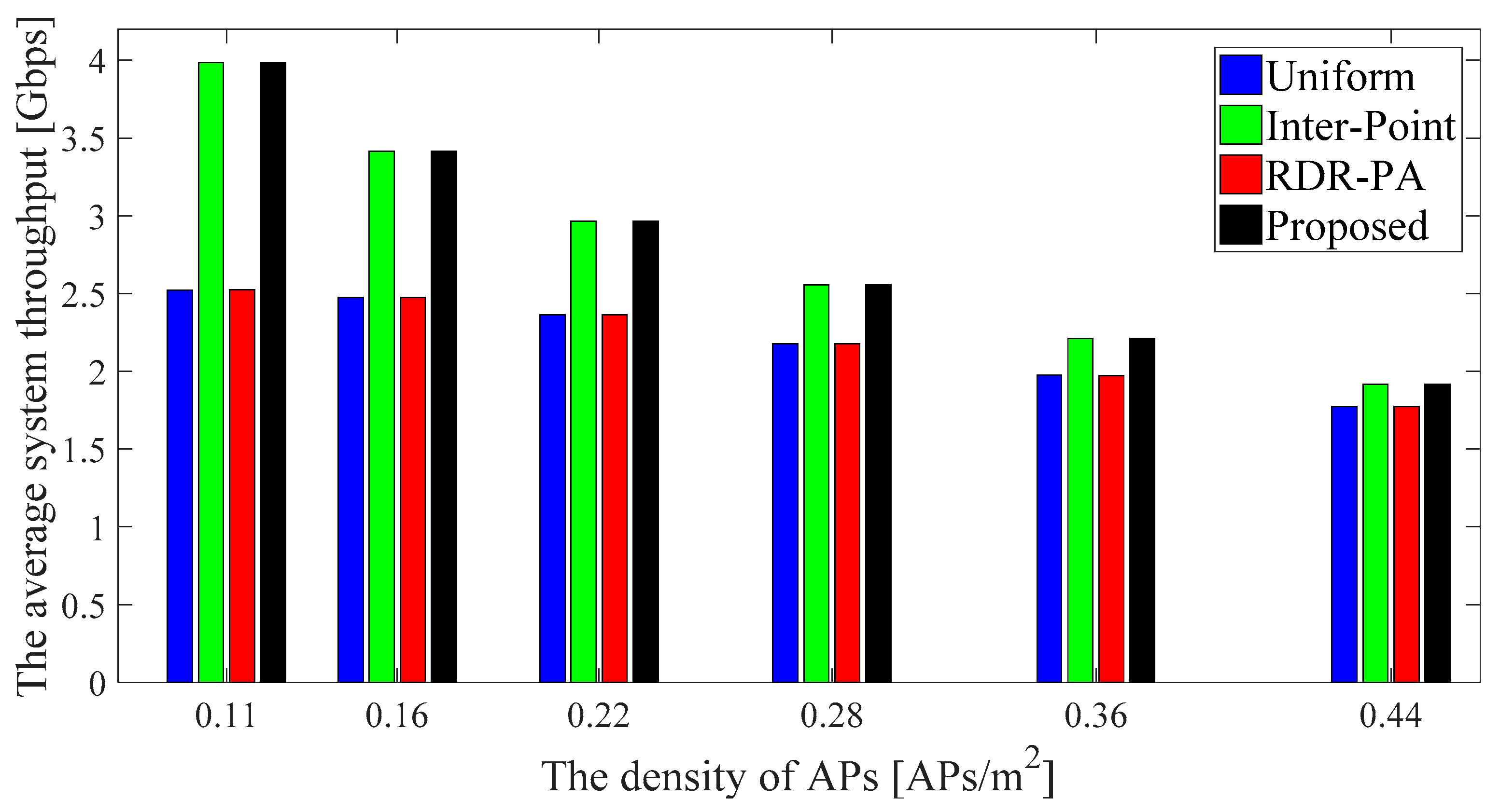
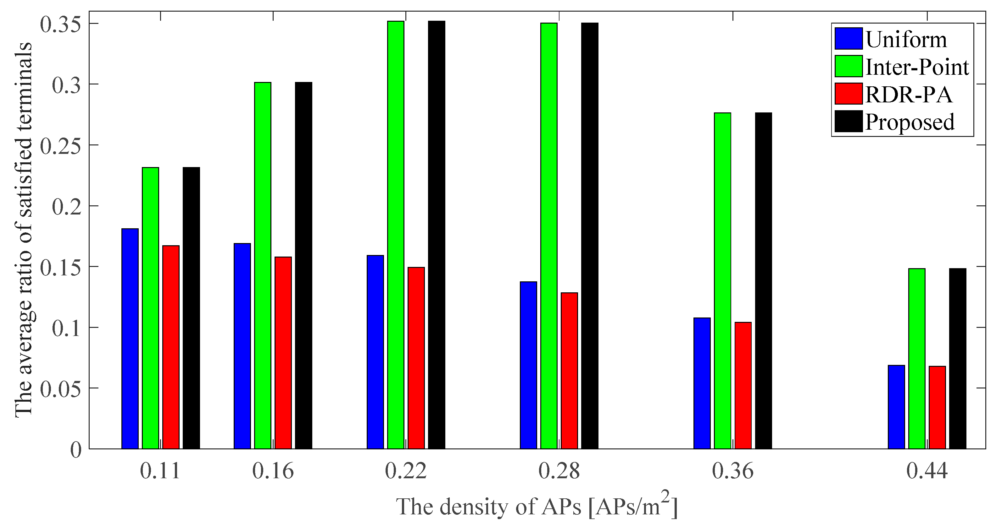
4.3. Analysis on Access Point Density
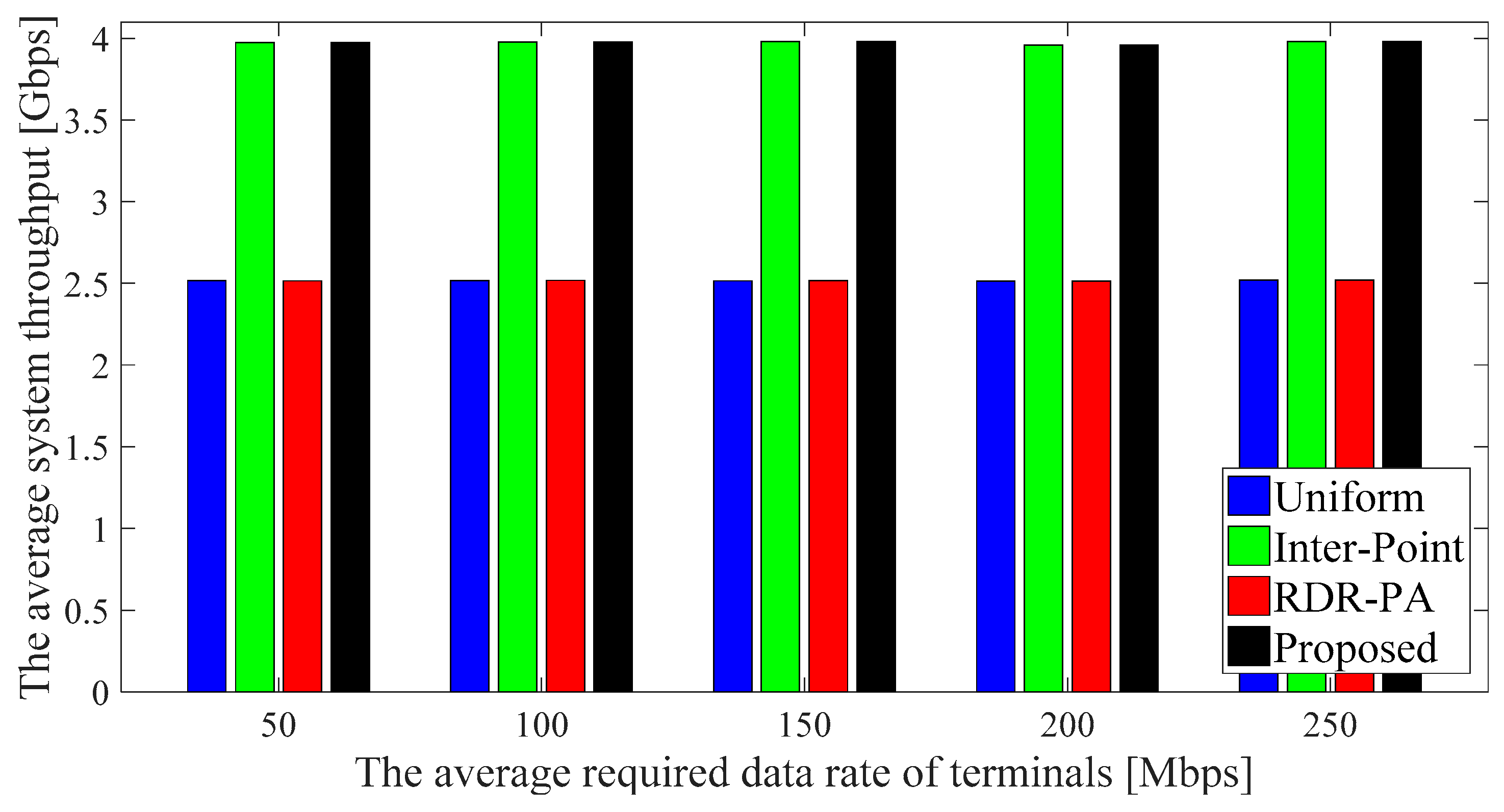
4.4. Analysis on Average Required Data Rate
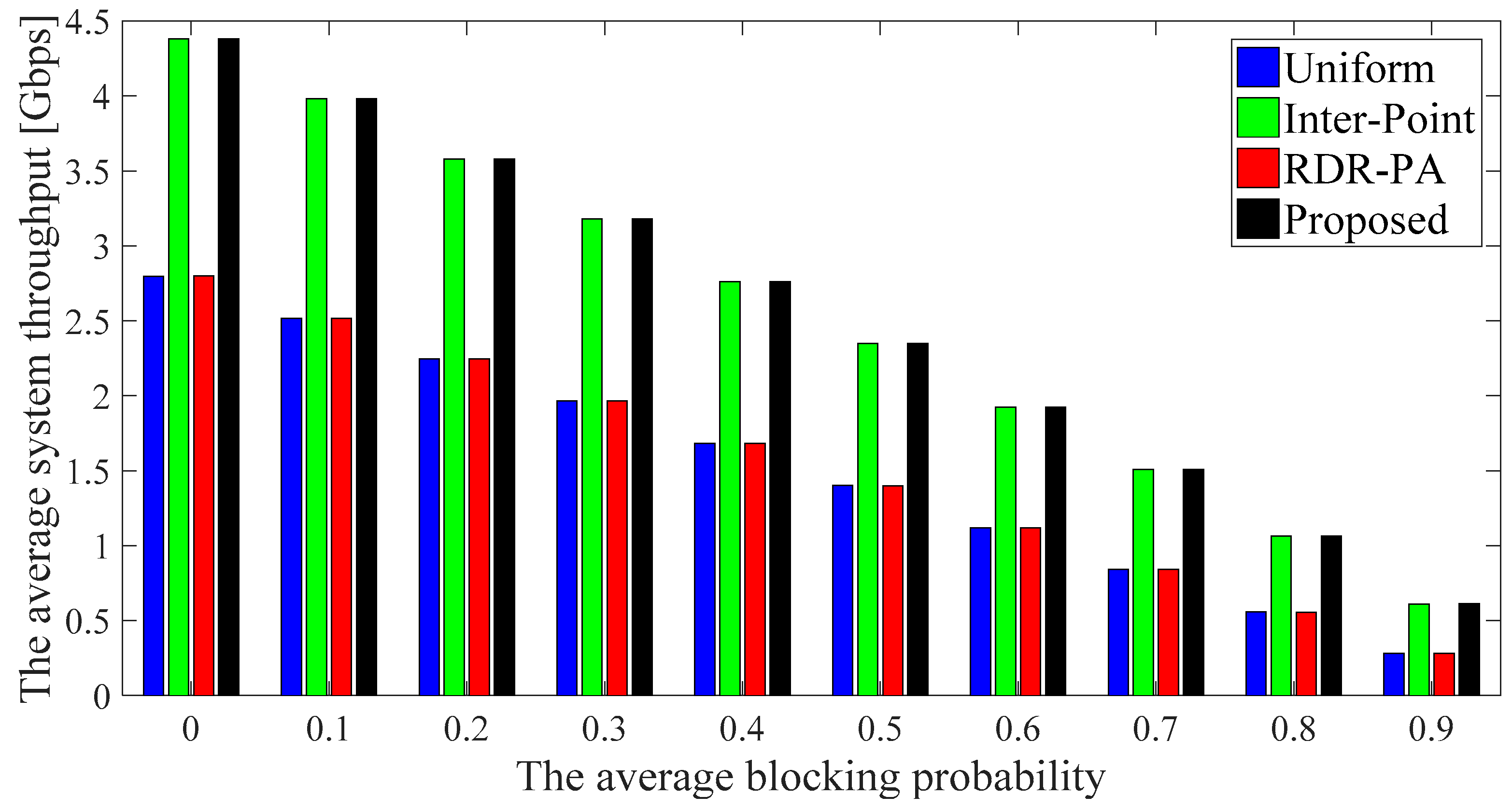
4.5. Analysis on Average Blocking Probability
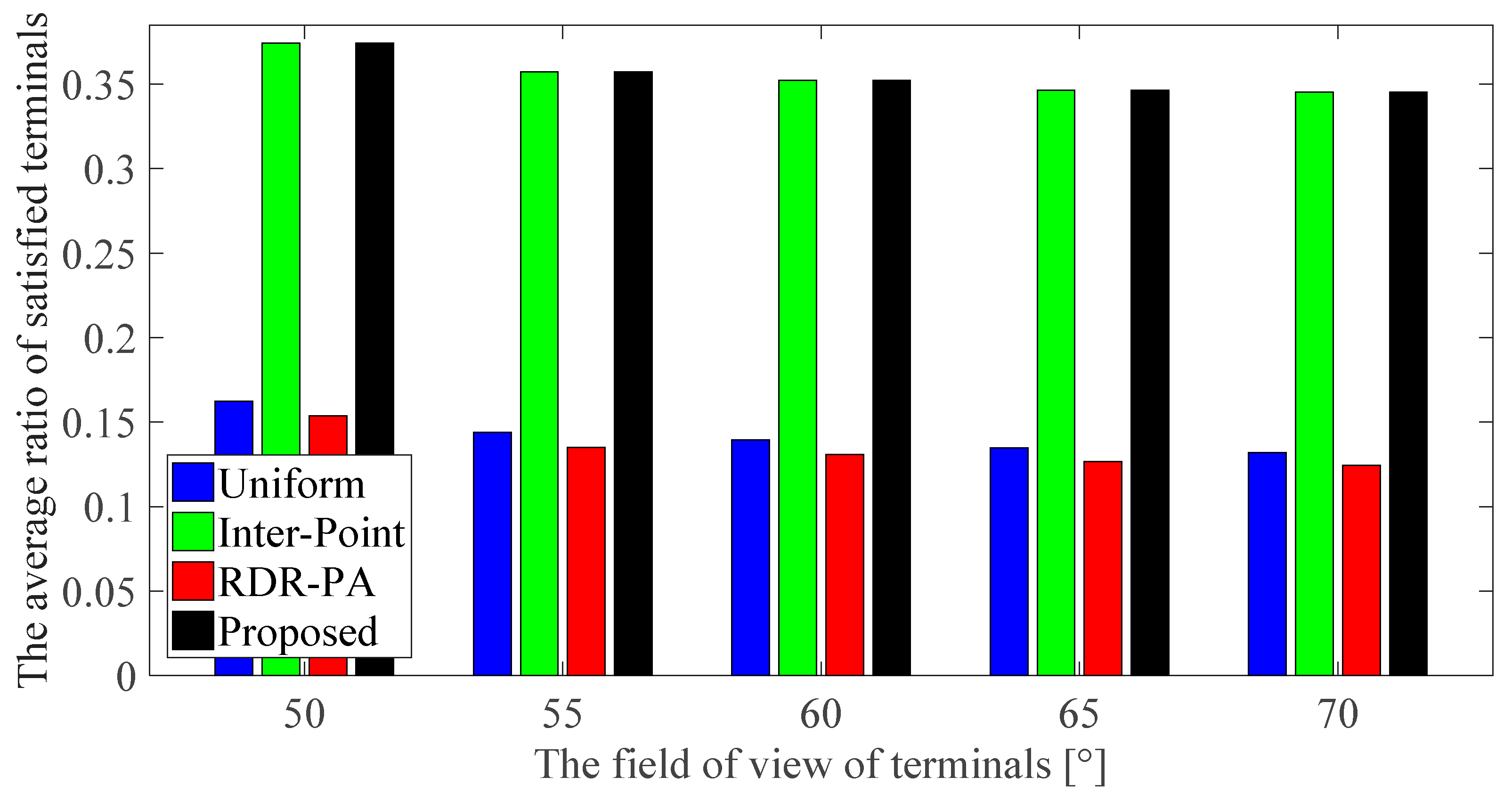
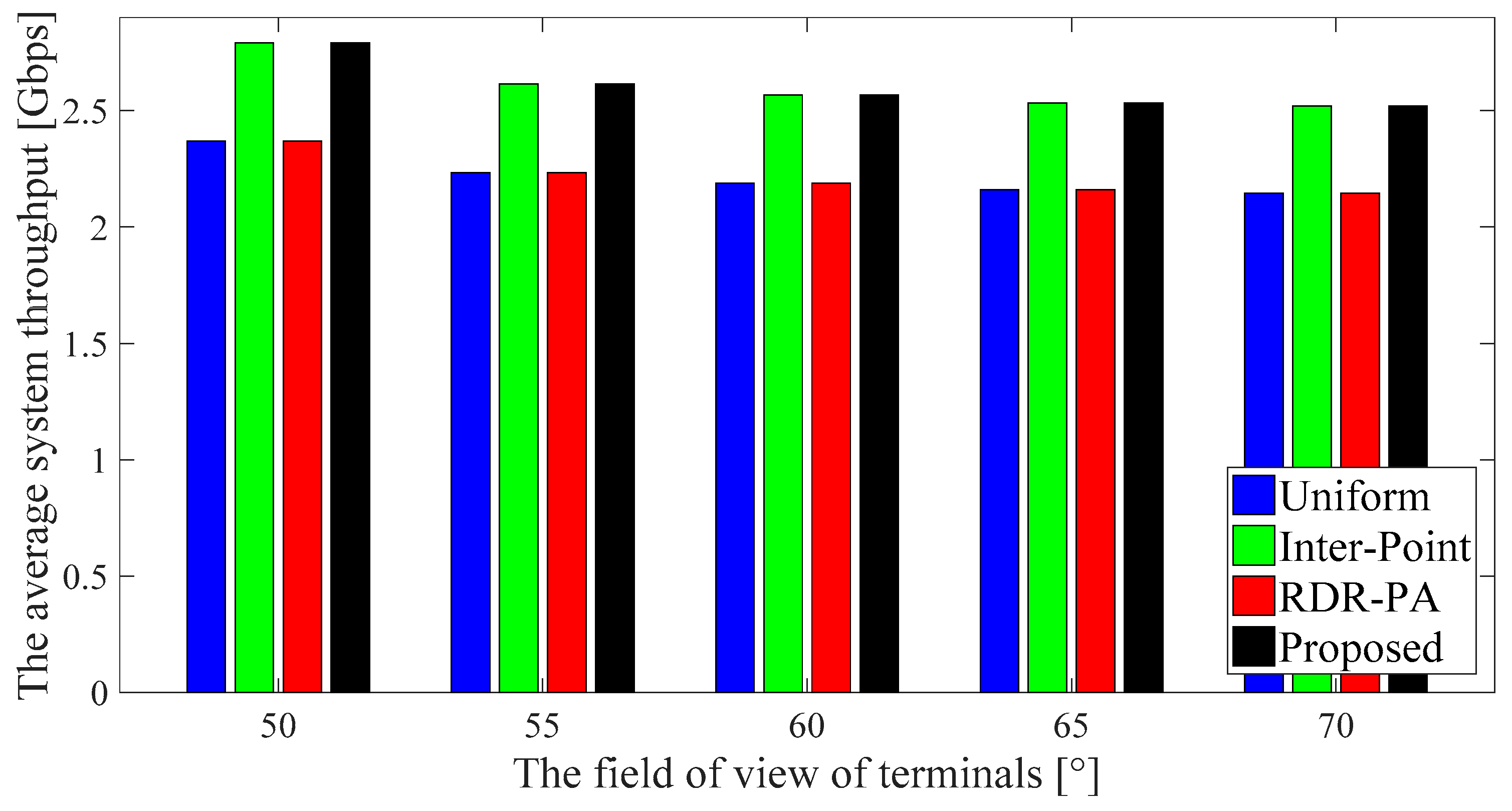
4.6. Analysis on Field of View
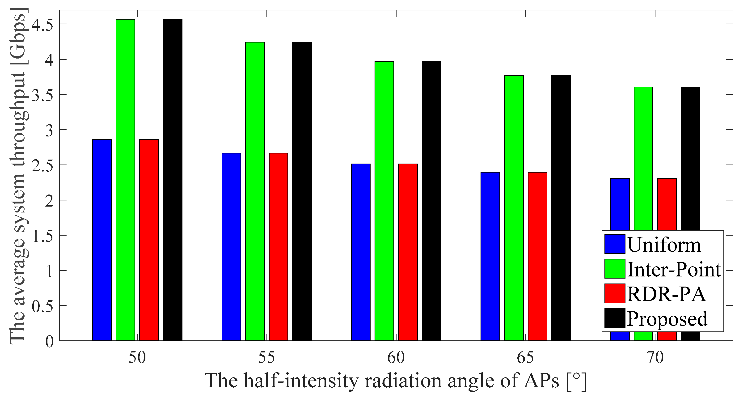
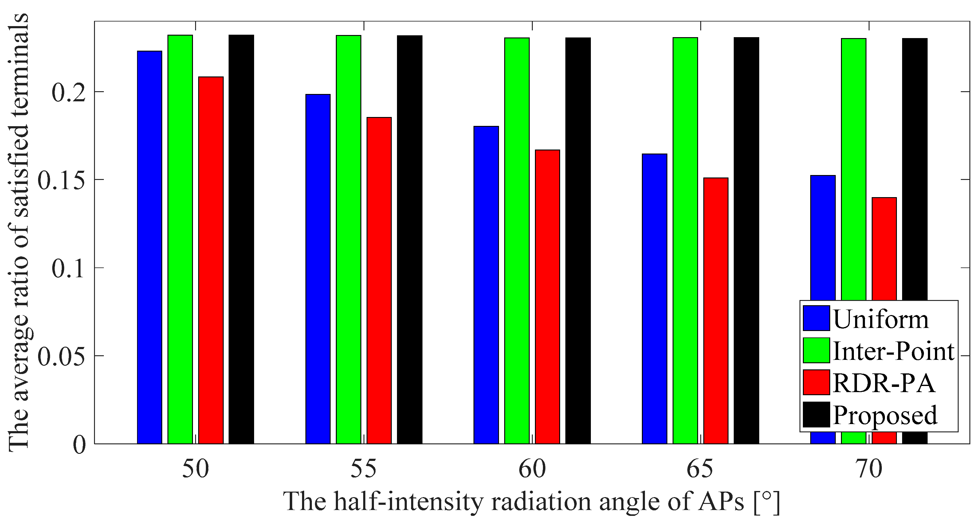
4.7. Analysis on Half-Intensity Radiation Angle
5. Conclusions
Author Contributions
Funding
Conflicts of Interest
References
- Li, X.; Jin, F.; Zhang, R.; Wang, J.H.; Xu, Z.Y.; Hanzo, L. Users first: User-centric cluster formation for interference-mitigation in visible-light networks. IEEE Trans. Wirel. Commun. 2016, 15, 39–53. [Google Scholar] [CrossRef]
- Zuo, Y.; Zhang, J.; Zhang, Y.Y.; Chen, R.H. Weight threshold check coding for dimmable indoor visible light communication systems. IEEE Photonics J. 2018, 10, 1–11. [Google Scholar] [CrossRef]
- Feng, L.F.; Hu, R.Q.; Wang, J.P.; Xu, P.; Qian, Y. Applying vlc in 5g networks: Architectures and key technologies. IEEE Netw. 2016, 30, 77–83. [Google Scholar] [CrossRef]
- Haas, H.; Yin, L.; Wang, Y.; Chen, C. What is lifi? J. Lightw. Technol. 2016, 34, 1533–1544. [Google Scholar] [CrossRef]
- Chen, C.; Serafimovski, N.; Haas, H. Fractional frequency reuse in optical wireless cellular networks. In Proceedings of the 2013 IEEE 24th Annual International Symposium on Personal, Indoor, and Mobile Radio Communications (PIMRC), London, UK, 8–11 September 2013; pp. 3594–3598. [Google Scholar]
- Li, X.; Huo, Y.K.; Zhang, R.; Hanzo, L. User-centric visible light communications for energy-efficient scalable video streaming. IEEE Trans. Green Commun. Netw. 2016, 1, 59–73. [Google Scholar] [CrossRef]
- Chen, S.; Qin, F.; Hu, B.; Li, X.; Chen, Z.; Liu, J. User-Centric Ultra-Dense Networks for 5G; Springer: Cham, Switzerland, 2018; p. 7. [Google Scholar]
- Li, X.; Zhang, R.; Wang, J.H.; Hanzo, L. Cell-centric and user-centric multi-user scheduling in visible light communication aided networks. In Proceedings of the 2015 IEEE International Conference on Communications (ICC), London, UK, 8–12 June 2015; pp. 5120–5125. [Google Scholar]
- Tao, S.Y.; Yu, H.Y.; Li, Q.; Tang, Y.Q. Performance analysis of gain ratio power allocation strategies for non-orthogonal multiple access in indoor visible light communication networks. EURASIP J. Wirel. Commun. Netw. 2018, 2018, 154. [Google Scholar] [CrossRef]
- Uddin, M.S.; Chowdhury, M.Z.; Jang, Y.M. Priority-based resource allocation scheme for visible light communication. In Proceedings of the 2010 Second International Conference on Ubiquitous and Future Networks (ICUFN), Jeju Island, Korea, 16–18 June 2010; pp. 247–250. [Google Scholar]
- Chowdhury, M.Z.; Uddin, M.S.; Jang, Y.M. Dynamic channel allocation for QoS provisioning in visible light communication. In Proceedings of the 2011 IEEE International Conference on Consumer Electronics (ICCE), Las Vegas, NV, USA, 9–12 January 2011; pp. 13–14. [Google Scholar]
- Chowdhury, M.Z.; Uddin, M.S.; Jang, Y.M. Dynamic channel allocation for class-based qos provisioning and call admission in visible light communication. Arab. J. Sci. Eng. 2013, 39, 1007–1016. [Google Scholar] [CrossRef]
- Chowdhury, M.Z.; Jang, Y.M.; Haas, Z.J. Priority based bandwidth adaptation for multi-class traffic in wireless networks. Int. J. Multimedia Ubiquitous Eng. 2014, 7, 445–450. [Google Scholar]
- Wu, X.; Safari, M.; Haas, H. Bidirectional Allocation Game in Visible Light Communications. In Proceedings of the 2016 IEEE 83rd Vehicular Technology Conference (VTC Spring), Nanjing, China, 15–18 May 2016; pp. 1–5. [Google Scholar]
- Wu, X.; Safari, M.; Haas, H. Three-state fuzzy logic method on resource allocation for small cell networks. In Proceedings of the 2015 IEEE 26th Annual International Symposium on Personal, Indoor, and Mobile Radio Communications (PIMRC), Hong Kong, China, 30 August–2 September 2015; pp. 1168–1172. [Google Scholar]
- Wu, X.; Safari, M.; Haas, H. Access point selection for hybrid li-fi and wi-fi networks. IEEE Trans. Commun. 2017, 65, 5375–5385. [Google Scholar] [CrossRef]
- Ibrahim, A.; Ismail, T.; Elsayed, K. Optimized radio resource allocation scheme for indoor optical wireless communication. In Proceedings of the 2017 19th International Conference on Transparent Optical Networks (ICTON), Girona, Spain, 2–6 July 2017; pp. 1–4. [Google Scholar]
- Wu, X.P.; Basnayaka, D.; Safari, M.; Haas, H. Two-stage access point selection for hybrid vlc and rf networks. In Proceedings of the 2016 IEEE 27th Annual International Symposium on Personal, Indoor, and Mobile Radio Communications (PIMRC), Valencia, Spain, 4–8 September 2016; pp. 1–6. [Google Scholar]
- Wang, Y.; Wu, X.; Haas, H. Fuzzy logic based dynamic handover scheme for indoor Li-Fi and RF hybrid network. In Proceedings of the 2016 IEEE International Conference on Communications (ICC), Kuala Lumpur, Malaysia, 22–27 May 2016; pp. 1–6. [Google Scholar]
- Kafafy, M.; Fahmy, Y.; Abdallah, M.; Khairy, M. Power efficient downlink resource allocation for hybrid rf/vlc wireless networks. In Proceedings of the 2017 IEEE Wireless Communications and Networking Conference (WCNC), San Francisco, CA, USA, 19–22 March 2017; pp. 1–6. [Google Scholar]
- Ye, C.; Gursoy, M.C.; Velipasalar, S. Quality-driven resource allocation for full-duplex delay-constrained wireless video transmissions. IEEE Trans. Commun. 2018, 66, 4103–4118. [Google Scholar] [CrossRef]
- Tian, W.; Liu, L.K.; Zhang, X.; Jian, C.X. A resource allocation algorithm combined with optical power dynamic allocation for indoor hybrid vlc and wi-fi network. In Proceedings of the 2016 8th International Conference on Computational Intelligence and Communication Networks (CICN), Tehri, India, 23–25 December 2016; pp. 21–27. [Google Scholar]
- Kahn, J.M.; Barry, J.R. Wireless infrared communications. Proc. IEEE 1997, 85, 265–298. [Google Scholar] [CrossRef]
- Liu, J.H.; Li, Q.; Zhang, X.Y. Cellular coverage optimization for indoor visible light communication and illumination networks. J. Commun. 2014, 9, 891–898. [Google Scholar] [CrossRef]
- Jin, F.; Zhang, R.; Hanzo, L. Resource allocation under delay-guarantee constraints for heterogeneous visible-light and rf femtocell. IEEE Trans. Wirel. Commun. 2015, 14, 1020–1034. [Google Scholar] [CrossRef]
- Bai, X.Y.; Li, Q.; Tao, S.Y. Resource allocation based on dynamic user priority for indoor visible light communication ultra-dense networks. In Proceedings of the 2018 IEEE 18th International Conference on Communication Technology (ICCT), Chongqing, China, 8–11 October 2018; pp. 331–337. [Google Scholar]
- Kashef, M.; Abdallah, M.; Qaraqe, K. Power allocation for downlink multi-user SC-FDMA visible light communication systems. Am. J. Trop. Med. Hyg. 2015, 77, 390–392. [Google Scholar]
- Burchardt, H.; Sinanovic, S.; Bharucha, Z.; Haas, H. Distributed and autonomous resource and power allocation for wireless networks. IEEE Trans. Commun. 2013, 61, 2758–2771. [Google Scholar] [CrossRef]
- Boyd, S.; Vandenberghe, L. Convex Optimization; Cambridge University Press: Cambridge, UK, 2004. [Google Scholar]
- Graham, R.L.; Knuth, D.E.; Patashnik, O. Concrete Mathematics: A Foundation for Computer Science, 2nd ed.; Addison-Wesley Publishing Company, Inc: Boston, MA, USA, 1994; pp. 443–448. [Google Scholar]
- Li, Y.R.; Huang, N.; Wang, J.Y.; Yang, Z.H.; Xu, W. Sum rate maximization for vlc systems with simultaneous wireless information and power transfer. IEEE Photonics Technol. Lett. 2017, 29, 531–534. [Google Scholar] [CrossRef]
- Xiao, Y.; Zhu, Y.J.; Zhang, Y.Y.; Sun, Z.G. Linear optimal signal designs for multi-color miso-vlc systems adapted to cct requirement. IEEE Access 2018, 6, 75519–75530. [Google Scholar] [CrossRef]


| Parameters | Value |
|---|---|
| Room size | 15 × 15 × 3 m3 |
| Transmit optical power of AP, Pt | 9 W |
| Vertical distance between the AP and terminal, | 2.15 m |
| Half-intensity radiation angle, | 60° |
| FOV of a receiver, | 60° |
| The refractive index, n | 1.5 |
| Detector responsivity, r | 0.53 A/W |
| The physical area of a receiver, A | 10−4 m2 |
| Power spectral density of noise, n0 | 10−21 A2/Hz |
| Bandwidth of each optical AP, B | 40 MHz |
| The gain of the optical filter, | 1 |
| Average required data rate, | 40 Mbps |
| Average blocking probability, | 0.1 |
| The access point density, | 0.11 APs/m2 |
| The terminal density, | 0.44 terminals/m2 |
© 2019 by the authors. Licensee MDPI, Basel, Switzerland. This article is an open access article distributed under the terms and conditions of the Creative Commons Attribution (CC BY) license (http://creativecommons.org/licenses/by/4.0/).
Share and Cite
Bai, X.; Li, Q.; Tang, Y. A Low-Complexity Resource Allocation Algorithm for Indoor Visible Light Communication Ultra-Dense Networks. Appl. Sci. 2019, 9, 1391. https://doi.org/10.3390/app9071391
Bai X, Li Q, Tang Y. A Low-Complexity Resource Allocation Algorithm for Indoor Visible Light Communication Ultra-Dense Networks. Applied Sciences. 2019; 9(7):1391. https://doi.org/10.3390/app9071391
Chicago/Turabian StyleBai, Xiangwei, Qing Li, and Yanqun Tang. 2019. "A Low-Complexity Resource Allocation Algorithm for Indoor Visible Light Communication Ultra-Dense Networks" Applied Sciences 9, no. 7: 1391. https://doi.org/10.3390/app9071391
APA StyleBai, X., Li, Q., & Tang, Y. (2019). A Low-Complexity Resource Allocation Algorithm for Indoor Visible Light Communication Ultra-Dense Networks. Applied Sciences, 9(7), 1391. https://doi.org/10.3390/app9071391