Abstract
Much of the current understanding of pharmaceutical pollution in the aquatic environment is based on research conducted in Europe, North America and other select high-income nations. One reason for this geographic disparity of data globally is the high cost and analytical intensity of the research, limiting accessibility to necessary equipment. To reduce the impact of such disparities, we present a novel method to support large-scale monitoring campaigns of pharmaceuticals at different geographical scales. The approach employs the use of a miniaturised sampling and shipping approach with a high throughput and fully validated direct-injection High-Performance Liquid Chromatography-Tandem Mass Spectrometry method for the quantification of 61 active pharmaceutical ingredients (APIs) and their metabolites in tap, surface, wastewater treatment plant (WWTP) influent and WWTP effluent water collected globally. A 7-day simulated shipping and sample stability assessment was undertaken demonstrating no significant degradation over the 1–3 days which is typical for global express shipping. Linearity (r2) was consistently ≥0.93 (median = 0.99 ± 0.02), relative standard deviation of intra- and inter-day repeatability and precision was <20% for 75% and 68% of the determinations made at three concentrations, respectively, and recovery from Liquid Chromatography Mass Spectrometry grade water, tap water, surface water and WWTP effluent were within an acceptable range of 60–130% for 87%, 76%, 77% and 63% of determination made at three concentrations respectively. Limits of detection and quantification were determined in all validated matrices and were consistently in the ng/L level needed for environmentally relevant API research. Independent validation of method results was obtained via an interlaboratory comparison of three surface-water samples and one WWTP effluent sample collected in North Liberty, Iowa (USA). Samples used for the interlaboratory validation were analysed at the University of York Centre of Excellence in Mass Spectrometry (York, UK) and the U.S. Geological Survey National Water Quality Laboratory in Denver (Colorado, USA). These results document the robustness of using this method on a global scale. Such application of this method would essentially eliminate the interlaboratory analytical variability typical of such large-scale datasets where multiple methods were used.
1. Introduction
Over the last 20 years, active pharmaceutical ingredients (APIs) and their metabolites have been identified in all environmental compartments and their occurrence has raised concerns over potential impacts on ecosystem and human health [1,2,3]. However, despite two decades of research, significant knowledge gaps exist regarding the environmental exposures to APIs [1,4]. For example, a complete or significant lack of knowledge exists for many parts of the world (e.g., Africa and South America) as such research disproportionally targets wealthy regions including North America, Western Europe and China [4,5]. In many poorly studied parts of the world, APIs are openly available without a prescription and prone to miss-/over-use so concentrations might be expected to be greater than those reported so far [6]. Similarly, API disposal practices and inefficient wastewater connectivity and treatment may further exacerbate high API concentrations in some regions [1,6]. Underpinning such research are the complex analytical methods employed for specific quantification of APIs in water, namely High-Performance Liquid Chromatography-Tandem Mass Spectrometry (HPLC-MS/MS). Such instrumentation is required for obtaining environmentally relevant sensitivity in measurements of APIs, down to ng/L levels.
The high cost of necessary instruments and analytical intensity of the methods employed are key barriers to broadening measurement of APIs in the environment to a global scale. Furthermore, such barriers may magnify existing regional disproportionalities in published data. Of the available published data, among the most significant challenges for compiling an international perspective on APIs in the aquatic environment is the cross-comparison between datasets obtained via different methodologies. Key areas of deviation between methodologies include sample collection protocols (e.g., collection from the river bank vs. centroid flow), analytical techniques and statistical/quantitative interpretations and use of quality-control samples throughout collection and analysis. No single, unified analytical method exists, and in-house method validations are not always required for publication, making accurate and reliable interpretations of existing data on concentrations of APIs in different regions of the globe challenging.
Recent advances in the sensitivity of analytical instrumentation provides the ability to now analyse a wide range of APIs with minimal sample pre-treatment (e.g., Furlong et al. [7]; Campos-Mañas et al. [8]. Direct-injection HPLC-MS/MS is characterised by large-volume sample injections (100–5000 μL) which eliminate the need for sample pre-concentration [9], traditionally achieved using solid phase extraction (SPE). This technique has been successfully used since the 1980s [9] and more recently employed for quantification of pharmaceuticals, illicit drugs and other organic contaminants in surface and wastewater [7,8,10]. Such methods significantly reduce the volume of sample needed (simplifying both sample collection and shipment to the laboratory) and the time for sample analysis via elimination of complex pre-treatment. Additionally, such methods offer a more environmentally responsible alternative to traditional methods (e.g., SPE) due to reduced sample volume and elimination of any need for solvents in sample pre-treatment. Direct-injection protocols also provide an opportunity to perform much larger-scale monitoring programmes than previously possible (e.g., due to financial and time constraints), allowing a better understanding of environmental exposures to pharmaceutical compounds (APIs and corresponding API metabolites) to aquatic systems around the globe. Conducting such large-scale global monitoring programmes will likely raise logistical challenges in terms of sample transport from the site of collection to the site of analysis. For these studies to succeed, therefore, it is important that sample integrity is maintained during such transport.
Here we present and evaluate a monitoring approach for use in large-scale monitoring programmes for APIs in multiple environmental matrices (e.g., WWTP influents, effluents, surface water and drinking water). The approach presents a simple and standardized set of protocols for the consistent collection, shipment, and analysis of aqueous samples using a uniform collection kit and a single HPLC-MS/MS analytical method. An interlaboratory evaluation of the protocol was conducted with surface water (i.e., river water) and WWTP effluent collected by the U.S. Geological Survey (USGS) from an effluent-impacted stream (Muddy Creek, North Liberty, Iowa, USA). This protocol may significantly reduce the challenges of: (a) evaluating spatial and temporal API concentration trends across variations in geography, climate, land use, hydrogeology, and demographics, (b) the lack of accessibility to costly analytical equipment and operating costs necessary for accurate and sensitive API quantification (namely HPLC-MS/MS) in some regions of the world, and (c) obtaining water samples from under-studied regions of the world for accurate, sensitive, reliable sample analysis. The development of this protocol therefore provides an opportunity to begin to better understand the risks of pharmaceuticals and other compounds at the global scale, a research priority highlighted in recent horizon scanning exercises on pharmaceuticals and chemicals more generally [5,11].
2. Materials and Methods
2.1. Test Substances
The protocol was developed for quantifying concentrations of 61 strategically selected APIs (Table 1) representing 19 therapeutic classes of medicinal chemicals approved for use in humans (n = 57) and animal husbandry (n = 4). The study APIs were selected to include: (a) compounds of high usage across the world; (b) compounds with known or suspected ecological or human health concern; and (c) compounds of expected high use due to regional disease pressures (e.g., antimalarials). Significant focus was placed on antimicrobial chemicals including antibiotics (n = 13) and antifungals (n = 6) due to implications for the selection of resistance to these medicines in bacterial communities [12,13]. Similarly, focus was also placed on antidepressants (n = 7) due to their increasing use globally and potential ecotoxicological risk [14]. All compounds were optimised for specific quantification using direct injection HPLC-MS/MS only and compounds not suitable for quantification using this instrumentation were not included in the study. Further method development may be used to broaden the scope of the studied contaminants (e.g., Campos-Mañas et al. [8]).

Table 1.
List of monitored chemicals by therapeutic class and their associated internal standard.
All test standards were purchased from Sigma Aldrich (UK) and were of ≥95% purity. Deuterated internal standards were obtained from Sigma Aldrich (UK) for 32 test APIs and atrazine-D5 was used where a labelled standard was not available. Liquid chromatography-mass spectrometry (LCMS)-grade water and methanol were obtained from VWR (UK). Polystyrene boxes (5 L, 34.5 × 21 × 14.5 cm, L × W × H) used for sample shipment were obtained from JB Packaging (Torpoint, UK), whereas 15-mL amber glass sample vials, 0.7-μm glass microfiber syringe filters (Whatman) and 24-mL luer lock syringes were obtained from Fisher Scientific (UK). A ZORBAX Eclipse Plus C18 chromatography column (3.0 × 100 mm, 1.8 μm, 600 bar) was purchased from Agilent Technologies (UK) and a C18 SecurityGuard guard column was purchased from Phenomenex (UK).
2.2. Sampling Kits and Water Collection Protocol
The sampling kits were designed to simplify logistics so that a large number of locations could be sampled with a minimum of effort. As the sample injection volume for the developed method was only 100 μL, the standard collection volume was set at 10 mL of sample water. Samples were collected in duplicate to provide a backup sample in case of breakage of the primary sample container during shipment. Each sampling kit therefore contained: 20 amber glass vials (15 mL) (for collection of 10 samples in duplicate), two ice packs, 10 polypropylene syringes (24 mL), 10 glass microfiber filters (0.7-μm pore size), a 500-mL stainless-steel bucket with 10-m long nylon cord attached, material to collect a field blank quality-control (QC) sample with LCMS-grade water, a standardised collection log and sample labels. Kits weighed 2.25 kg and were able to fit into a 34.5 × 21 × 14.5 cm box (approximately the size of a shoe box).
The sample collection protocol, including storage and shipping procedures, was included with the sampling kit and instructional videos were also provided online (<https://youtu.be/HeZ7xoxJXhM> and <https://youtu.be/PLyCNcVCKdc>). At each location, the bucket (included with each kit) was rinsed three times with native sample water prior to collection. Following sample collection, 20 mL of sample water was aspirated into the syringe, and the syringe filter was then attached and primed with 5 mL of sample water. Then, 5 mL of filtrate was used to rinse out a 15-mL vial prior to dispensing the remaining 10 mL of filtrate into the glass vial. This procedure was repeated once more with the same bucket of water to create the second replicate. At this point, pH, temperature or other probes may be inserted into the water remaining in the bucket to obtain additional environmental data. All vials were labelled with their location, sample date/time, and replicate number and immediately placed on ice upon collection. Prior to shipment, samples were frozen until being shipped on ice to the University of York (York, UK) Centre of Excellence in Mass Spectrometry (CoEMS) using DHL global express delivery (1–2 days). Freezing the samples prior to express shipping to CoEMS ensured the samples maintained their integrity (i.e., did not become warm during shipment) prior to analysis.
2.3. HPLC-MS/MS Protocol
The analytical method was adapted from a previously developed method for pharmaceuticals compounds [7]. Analysis occurred by direct-injection (100-µL injection volume) HPLC-MS/MS in multiple reaction monitoring (MRM) mode with positive electrospray ionisation. A Thermo Scientific Endura TSQ triple quadrupole mass spectrometer coupled with a Thermo Scientific Dionex UltiMate 3000 HPLC was used for all analyses. Two transition ions were optimised (for collision energy and retention time) in-house, one for quantitation (T1) and another for confirmation (T2) of precursor identity (Table S1). The instrument-calibrated fragmentor voltage was used for all analysis. Mobile phase A was LCMS-grade water with 0.01 M formic acid and 0.01 M ammonium formate while mobile phase B was 100% methanol. The flow rate was 0.45 mL/min. Flow was diverted away from the spectrometer for the first 1 min of the analytical run to avoid poorly retained materials (e.g., slats) from reaching the nebuliser. The HPLC gradient started at 10% B which increased to 40% at 5 min, 60% at 10 min, and 100% at 15 min, where it remained until 23 min then reduced to 10% at 23.1 min prior to a 10-min re-equilibration time between runs. Autosampler temperature was maintained at 6 °C while the column temperature was maintained at 40 °C. The collision gas was argon and was set at a pressure of 2 mTorr. Quantification occurred using a 15-point calibration prepared for 33 deuterated internal standards (Table 1, Table S1) ranging from 1 to 8000 ng/L (Table S2). All calibrants were made using a standard method as described by Furlong et al. [7] in such a way as to maintain an equal proportion of methanol in the final calibrants (Table S2). Atrazine-D5 was used where a labelled standard was not available for a specific target chemical, as established by Furlong et al. [7].
2.4. Quality Control
Extensive quality-control measures were used in-house and in the field to ensure that the laboratory and field protocols were not causing false positives or negatives in the corresponding environmental results. Materials needed to conduct one field blank were included in each sample kit which included 25 mL of LCMS-grade water, a syringe filter, syringe and two 15-mL glass vials. The procedure for collection, storage and shipment of this QC sample was exactly the same as for environmental samples, except using LCMS-grade water. This step enables an evaluation of sample contamination derived from collection in the field.
In addition to field QC measures, a blank as well as method and instrumental QCs were injected after every 10 injections during analytical runs. The laboratory blanks were pure LCMS-grade water with all internal standards spiked to a concentration of 400 ng/L. Both method and instrumental QCs consisted of all target APIs spiked in LCMS-grade water at a concentration of 80 ng/L with all QCs at 400 ng/L. However, the method QC underwent the same sample storage and preparation measures as actual samples and the instrumental QC was spiked directly into a HPLC vial prior to analysis. Before each use, the nebuliser and spray guard of the mass spectrometer were cleaned with methanol. Additionally, prior to an analytical run, the chromatography column was equilibrated with 20 injections of a composite environmental sample (made from equal aliquots of the samples being analysed in respective runs) in order to condition the chromatography column prior to analysis.
2.5. Method Validation
The method was validated based on USGS method No. O-2440-14 (National Water Quality Laboratory [NWQL] laboratory schedule 2440) for filtered water [7], which will be referred to as USGS method No. 5-B10 in this paper. Briefly, intra-/inter-day repeatability was determined at three concentrations (10, 100 and 1000 ng/L) over 3 days (n = 10 per concentration). Analyte response (recovery) was also determined at three concentrations (10, 100 and 1000 ng/L) in LCMS-grade water, drinking water directly from the tap (chlorinated), surface water, and WWTP influent and effluent. Surface water was obtained from the River Ouse in York City Centre (UK, GPS coordinates: 53.957397, −1.083816), drinking water was from the tap at the University of York (York, UK), and both WWTP influent and effluent were obtained from a WWTP in Barnsley, UK. Limits of detection (LOD) and quantification (LOQ) were statistically derived using the method described by Sallach et al. [15]. Briefly, respective LODs were based on the Grubbs t-test constant for 10 variables multiplied by the standard deviation of 10 replicate quantifications of test chemicals in mixture at the lowest calibrant level (1 ng/L). The LOQs for respective analytes were determined as two times the LOD [15]. Analytical limits were determined in LCMS-grade water, drinking water, surface water, and WWTP influent and effluent. An acceptable range for analyte response was considered between 60–130% and <20% for intra-/inter-day repeatability and precision as established by USGS method No. 5-B10 [7].
2.5.1. Evaluation of Chemical Stability
To evaluate the potential degradation of test APIs during shipment, a stability assessment was performed at three temperatures: 4 °C (n = 6), 20 °C (n = 6), and 35 °C (n = 6) (Table S3). Six replicates of 10-mL LCMS-grade water for each temperature were spiked with a mixture of all test chemicals to make a final mixed concentration of all the APIs at 1000 ng/L. Samples were then stored at the designated temperatures for either 2 or 7 days to provide the range of holding times from the field to the laboratory that would be encountered for this protocol. A 1-mL aliquot of each sample was collected, and analysis occurred via the same procedure as environmental samples. In addition to the stability assessment to assess if sample storage temperature during shipping affects API concentrations, the interior temperature of three sets of polystyrene packages containing two ice packs frozen at −20 °C was measured over 7 days to determine the conditions samples are likely to experience during shipment.
2.5.2. Interlaboratory Assessment
To validate the method using independent analytical results, an interlaboratory comparison was conducted where four samples (three stream samples and 1 WWTP effluent sample) were simultaneously collected for API analysis at CoEMS and the USGS using USGS method No. 5-B10 [7]. Both methods used the exact same field sample processing procedures and materials (e.g., 15-mL amber glass sample vials, 24-mL leur lock syringes, and 0.7-µm glass microfiber syringe filters) making for a more effective comparison of the analytical methods used without having added variability due to field collection and processing procedures. All samples for this interlaboratory comparison (Figure S1) were collected from Muddy Creek, North Liberty, Iowa (USA) using the provided sampling kit and designated protocols and were immediately chilled and express mailed the same day as sample collection and arriving within 24 h to the USGS NWQL in Denver (Colorado, USA) for analysis. Samples to CoEMS were frozen following collection and then express mailed where they were received within 37 h still frozen. There were 30 overlapping APIs between these two methods for this interlaboratory comparison (Table S4). USGS method No. 5-B10 uses the same chromatography column, injection volume and positive ESI as the CoEMS method, however it is conducted using an Agilent Technologies 6460 triple quadrupole tandem mass spectrometer coupled to an Agilent 1200 HPLC system [7]. The data were evaluated based on their absolute difference (%) and the order (from highest concentration to lowest) of quantified APIs.
3. Results and Discussion
3.1. Method Validation
All of the validated API parameters were assessed against the range established by USGS method No. 5-B10 (matrix recovery of 60–130% and RSD ≤20%) and the determined analytical limits (Table 2) were all in the ng/L range [7]. Mean calibration r2-values were 0.984 ± 0.019, relative standard deviation of intra- and inter-day repeatability and precision was typically ≤20% (Table S5), and recovery from LCMS-grade water (Table S6), tap water (Table S7), surface water (Table S8), WWTP effluent (Table S9) and WWTP influent (Table S10) were typically between 60–130%. Analyte response (i.e., recovery) was comparable between LCMS-grade water, drinking water and surface water with deviation from a range of 60–130% most notable in WWTP influent (67% of determinations). This is likely due to matrix enhancement and indicates that analysis of WWTP influent may be best conducted with an initial sample clean-up method or by analysis following dilution of the sample using methods described by Furlong et al. [7]. Limits of detection were lowest in LCMS-grade water and highest in WWTP influent (Table S11). Generally, little difference was observed between the analytical limits determined in LCMS-grade water and those in tap and surface water enabling sensitive use of the method with these matrices (Table 2).
Table 2.
Statistical overview of method validation showing the mean value and standard deviation (SD) for each parameter and the percent of determinations which fall between the acceptable range employed by U.S. Geological Survey (USGS) Method No. 5-B10.
This validation indicates that the method presented here is sufficiently robust and is best used in high-throughput applications for analysis of drinking and surface water. The method can also be applied with reasonable accuracy in non-diluted WWTP effluent. While analysis of influent water is possible, dilution is recommended on a site-specific basis due to potential matrix effects. The precision of the analysis in influent samples may be improved with further sample pre-treatment such as solid phase extraction [16].
The analytical response and limits demonstrated by this method are comparable to (e.g., Furlong et al. [7], Oliveira et al. [17], Hermes et al. [18]) and more sensitive than (e.g., Campos-Mañas et al. [8]) other direct-injection HPLC-MS/MS methods. This supports similar work demonstrating that direct-injection HPLC-MS/MS can achieve robust and specific quantification at low ng/L levels without a need for sample clean-up (other than filtration) and pre-concentration [16]. Furthermore, this method provides similar environmentally relevant sensitivity as more rigorous (and likely more expensive) protocols involving sample pre-concentration and SPE (e.g., Gurke et al. [19], Paiga et al. [20]). The protocol presented here also offers a clear advantage over others as the shipment and chemical stability of the selected contaminants during shipment was also validated, as shown in Section 3.2. Therefore, use of this protocol allows for sample collection in areas geographically isolated from analytical centres, which may reduce the accessibility barriers to sensitive analytical equipment worldwide.
3.2. Evaluation of Chemical Stability during Shipment
Simulated shipping events (n = 3) showed that the interior temperature of the polystyrene package remained below ambient temperature for 2.44 days (Figure 1). A negative relationship between chemical stability in water and both temperature and time was observed, and degradation was consistently higher with increasing temperature and time. Over 2 days, the degradation study determined a mean stability of 92% ± 8.6% at 4 °C, 89% ± 7.9% at 20 °C and 90% ± 13% at 35 °C. After 7 days at respective temperatures, stability dropped to 83% ± 11%, 80% ± 13% and 77% ± 19% at 4 °C, 20 °C and 35 °C respectively (Figure 2, Table S3).
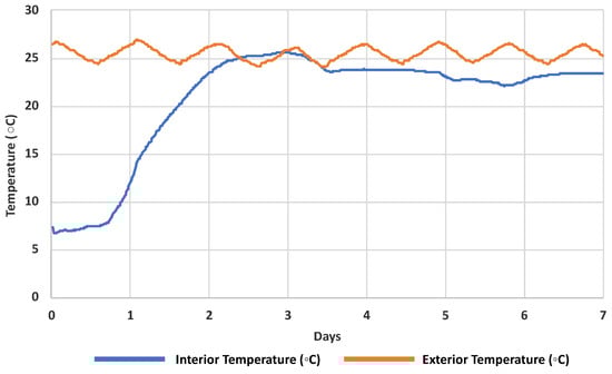
Figure 1.
Mean (n = 3) interior and exterior temperatures of a sample shipping package containing two ice packs (as standardised for all sampling kits) over 7 days.
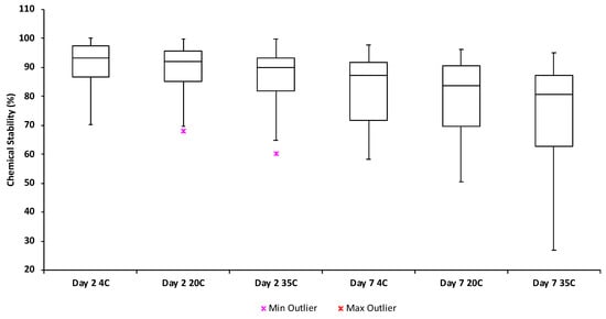
Figure 2.
Stability of the target chemicals in liquid chromatography-mass spectrometry (LCMS)-grade water held at 4 °C, 20 °C and 35 °C for 2 and 7 days respectively.
Fluoxetine and its metabolite norfluoxetine were the least stable, exhibiting a mean degradation of 29.7–37.5% and 29.3–34.2% respectively over 2 days and 41.2–50.3% and 41.6–49.2% respectively over 7 days (Table S3). Interestingly, previous work has indicated that both fluoxetine and norfluoxetine are relatively hydrolytically stable [21]. However, they are known to rapidly partition to solid matrices such as sediment [22]. Hence, the decreased stability of these chemicals observed here may partially be an artefact of sorption to test materials including the glass test vessel/PTFE cap or plastic pipette tips. The tetracycline antibiotics tetracycline and oxytetracycline were also relatively unstable exhibiting mean degradation of 20.9–24.2% and 21.1–29.3% respectively after 2 days and 34.8–43.1% and 32.3–39.3% respectively after 7 days (Table S3). Previous work has indicated that both tetracycline and oxytetracycline are quickly degradable via oxidation (e.g., Jeong et al. [23]). Despite the observed degradation, the dissipation of fluoxetine, norfluoxetine and the tetracyclines were still of an acceptable level to draw conclusions over the relative fate and abundance of these contaminants in water. All remaining test chemicals generally demonstrated degradation of <20% over 2 days and <30% over 7 days (Table S3).
As express shipping usually takes 1–2 days and samples are shipped frozen, it is unlikely that any API in this method would significantly degrade during shipment. Here, a mean degradation rate of 11% ± 7.9% (median degradation of 9.1%) over 2 days at 20 °C (Table S3) is superior to the typical loss of 20–40% on sample pre-treatment steps not required by this method (e.g., solid phase extraction) from water at environmentally relevant pH levels [20,24].
3.3. Interlaboratory Assessment
The 30 overlapping APIs between the CoEMS and USGS methods led to 120 chemical determinations for comparison, with chemical results being confirmed in 98% of determinations (117 of 120, Table S4). Only three determinations for codeine were confirmed at low concentrations (i.e., 15 to 26 ng/L) via the USGS method while not detected by the CoEMS method (Table S4). Of the 120 total determinations, 48 were nondetects in both methods, 14 were not detected in one method but confirmed between the LOD and LOQ of the other (e.g., mainly due to differences between LODs), 55 determinations were confirmed and quantified in both methods, while three were confirmed and quantified in one method but not in the other (Table S4).
The 55 determinations which were confirmed and quantified by both methods covered 19 APIs (Figure 3). Concentrations determined between the methods were in agreement with an overall mean deviation of 19.5% ± 12.3% (Figure 3). Within this deviation, 76.4% of the determinations made at CoEMS were lower than those determined by the USGS (mean 19.6% ± 9.6% lower). No substantial difference was observed between the interlaboratory deviations in WWTP effluent and surface water with median discrepancies of 19.7% (31.5 ng/L) and 19.4% (37.9 ng/L) respectively. The absolute differences in respective matrices ranged from 2.4% (1 ng/L, trimethoprim) to 38.7% (31.5 ng/L, sitagliptin) in effluent and 0.8% (2.6 ng/L, tramadol) to 36.4% (104 ng/L, lidocaine) in surface water (Figure 3). Generally, deviation between the two values (Table S4) was within the intra-day repeatability of the CoEMS method (Table S5).
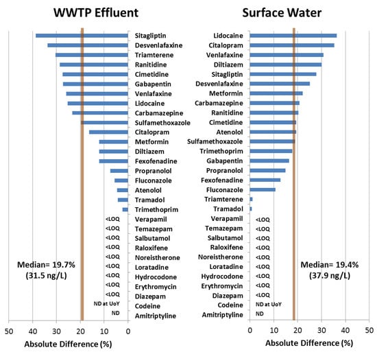
Figure 3.
Relative percent difference (RPD) between concentrations of 30 medicinal chemicals (present in both respective methods) quantified by the USGS (using USGS method No. 5-B10 [7]) and CoEMS (using the method presented in this work) in both WWTP effluent and surface water with median RPD represented by the vertical bar.
The top five APIs prioritised by concentration in both WWTP effluent and surface water were identical for both the USGS and CoEMS assessments: Fexofenadine, gabapentin, metformin, desvenlafaxine and venlafaxine (Figure 4).
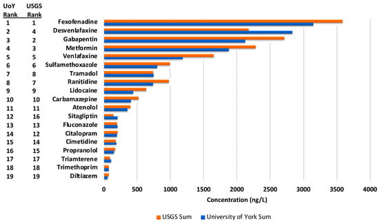
Figure 4.
Sum concentrations of the 19 quantified active pharmaceutical ingredients (APIs) determined by analysis at the CoEMS and USGS respectively with their prioritisation rank determined by total concentration.
3.4. Concentrations of Studied APIs in Muddy Creek
Of the 61 APIs in the presented method, 31 were detected in at least one sample from Iowa (Table S12). The highest number of APIs was detected in the WWTP effluent sample (n = 31) and the lowest (n = 16) in the stream sample collected upstream of the WWTP discharge point. The fluoroquinolones ciprofloxacin and enrofloxacin were the only APIs detected above quantification levels in the upstream sample (54.3 and 185.6 ng/L respectively), potentially due to upstream agricultural pressures or other urban sources (e.g., leaking sewer lines or septic systems). The total API concentration was lowest upstream of the WWTP (239.9 ng/L), highest in the WWTP effluent (10,373 ng/L) and attenuated (from 5561.5 to 3699.4 ng/L) with increasing distance downstream from the WWTP outfall (Figure 5) as one would expect in an effluent-dominated system [25]. At the time of sampling, 55% of Muddy Creek flow downstream from the WWTP consisted of sewage plant effluent. The composition of the detected APIs in Muddy Creek was clearly defined by those in the WWTP effluent and was dominated by antihistamines > antidepressants > antiepileptics > and antihyperglycemics (Figure 5). The API detected at the highest concentration was the antihistamine fexofenadine at a maximum concentration of 1644 ng/L in the effluent and 926 ng/L in surface water collected downstream of the WWTP (Table S4). This was closely followed by the antidepressant desvenlafaxine in the WWTP effluent with a concentration of 1617 ng/L. Interestingly, this chemical is also an active metabolite of the antidepressant venlafaxine, which was detected at 681.3 ng/L in the same effluent sample.
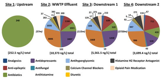
Figure 5.
Muddy Creek study sites by proportion of detected therapeutic class of the 61 target APIs in the presented method with [site total concentration] and (distance between sites in meters). Pie charts are labelled with the total detected concentration (ng/L) of APIs belonging to respective therapeutic classes.
3.5. Implication for Future Research
The method presented here offers the first truly transferable sampling, shipping and mass spectrometry protocol for use in global monitoring campaigns. Potential applications include research extending the spatial and temporal resolution of published data on API contamination of water globally, applications related to antimicrobial resistance selection, as well as the potential for further method development enabling determination of other aquatic contaminants including persistent organic pollutants and metals. The small size of the sample vials and corresponding shipping packages and ease of sample collection may encourage the incorporation of citizen science in future API research. Fast, easy and cheap analytical methods are key to advancing the understanding of exposure to chemical contaminants via water and this method offers a clear step forward.
Supplementary Materials
Supplementary tables and figures are available online at: https://www.mdpi.com/2076-3417/9/7/1368/s1. Figure S1: Map of the sampling locations along Muddy Creek with GPS coordinates and sample site description, Table S1: Mass spectrometer conditions and target ions with precursor, transition 1 (T1) for quantitation and transition 2 (T2) for confirmation mass-to-charge ratios, collision energy and retention times, Table S2: Concentrations of the 15 calibration levels used in this method with the volumes and concentrations of mixed stock solutions used to create final calibrants with an equal amount of organic solvent in each, Table S3: Stability of monitored chemicals over 2 and 7 days at three temperatures, Table S4: Concentrations of 30 medicinal chemicals quantified in Muddy Creek (Iowa, USA) by the USGS (Central Midwest Water Science Center, Iowa City, Iowa) and University of York (York, UK), Table S5: Linearity (n = 3) and relative standard deviation (%) of both Intra-day repeatability (n = 6) and intermediate precision (n = 6) for the 61 APIs in the presented method validation with cells shaded in red indicating RSD > 20%, Table S6: Recovery (%) of 61 APIs from LCMS-grade water (n = 10) with cells shaded in green indicating a recovery between 60–130%, Table S7: Recovery (%) of 61 APIs from drinking (tap) water obtained from the University of York (n = 10) with cells shaded in green indicating a recovery between 60–130%, Table S8: Recovery (%) of 61 APIs from surface water obtained from the River Ouse in York City Centre, UK (n = 10) with cells shaded in green indicating a recovery between 60–130%, Table S9: Recovery (%) of 61 APIs from wastewater treatment plant (WWTP) effluent obtained from a WWTP in Barnsley, UK (n = 10) with cells shaded in green indicating a recovery between 60–130%, Table S10: Recovery (%) of 61 APIs from wastewater treatment plant (WWTP) influent obtained from a WWTP in Barnsley, UK (n = 10) with cells shaded in green indicating a recovery between 60–130%, Table S11: Limits of Detection (LOD) and Quantification (LOQ) determined in respective matrices, Table S12: Concentrations, in ng/L, of all 61 APIs determined by the method presented in this paper found in the Muddy Creek (North Liberty, Iowa, USA).
Author Contributions
J.L.W.: Co-conception of the idea, sample analysis, data analysis, data interpretation, writing of the manuscript and editing; A.B.A.B.: Co-conception of the idea, data interpretation, writing of the manuscript and editing. D.W.K.: Sample collection/analysis, data analysis, data interpretation and editing.
Funding
This research received no external funding.
Acknowledgments
The authors would like to thank Shannon Meppelink and Jessica Garret (USGS Central Midwest Water Science Center) for the collection of stream and WWTP effluent samples at the Muddy Creek sites and programmatic support by the Toxic Substances Hydrology Program of the USGS Environmental Health Mission Area. Any use of trade, product, or firm names is for descriptive purposes only and does not imply endorsement by the U.S. Government. The authors also acknowledge the York CoEMS which was created thanks to a major capital investment through Science City York, supported by Yorkshire Forward with funds from the Northern Way Initiative, and subsequent support from EPSRC (EP/K039660/1; EP/M028127/1).
Conflicts of Interest
The authors declare no conflict of interest.
References
- aus der Beek, T.; Weber, F.A.; Bergmann, A.; Hickmann, S.; Ebert, I.; Hein, A.; Küster, A. Pharmaceuticals in the environment—Global occurrences and perspectives. Environ. Toxicol. Chem. 2016, 35, 823–835. [Google Scholar] [CrossRef]
- Parthasarathy, R.; Monette, C.E.; Bracero, S.; Saha, M.S. Methods for field measurement of antibiotic concentrations: Limitations and outlook. FEMS Microbiol. Ecol. 2018, 94, 105. [Google Scholar] [CrossRef] [PubMed]
- Tisler, S.; Zwiener, C. Formation and occurrence of transformation products of metformin in wastewater and surface water. Sci. Total Environ. 2018, 628, 1121–1129. [Google Scholar] [CrossRef]
- Hughes, S.R.; Kay, P.; Brown, L.E. Global synthesis and critical evaluation of pharmaceutical data sets collected from river systems. Environ. Sci. Technol. 2012, 47, 661–677. [Google Scholar] [CrossRef] [PubMed]
- Van den Brink, P.J.; Boxall, A.B.; Maltby, L.; Brooks, B.W.; Rudd, M.A.; Backhaus, T.; Spurgeon, D.; Verougstraete, V.; Ajao, C.; Ankley, G.T.; et al. Toward sustainable environmental quality: Priority research questions for Europe. Environ. Toxicol. Chem. 2018, 37, 2281–2295. [Google Scholar] [CrossRef] [PubMed]
- Hossain, A.; Nakamichi, S.; Habibullah-Al-Mamun, M.; Tani, K.; Masunaga, S.; Matsuda, H. Occurrence and ecological risk of pharmaceuticals in river surface water of Bangladesh. Environ. Res. 2018, 165, 258–266. [Google Scholar] [CrossRef]
- Furlong, E.T.; Noriega, M.C.; Kanagy, C.J.; Kanagy, L.K.; Coffey, L.J.; Burkhardt, M.R. Determination of Human-Use Pharmaceuticals in Filtered Water by Direct Aqueous Injection: High-Performance Liquid Chromatography/Tandem Mass Spectrometry. U.S. Geological Survey Techniques and Methods 5-B10. 2014. Available online: https://pubs.usgs.gov/tm/5b10/pdf/tm10-b5.pdf (accessed on 8 March 2019).
- Campos-Mañas, M.C.; Plaza-Bolaños, P.; Sánchez-Pérez, J.A.; Malato, S.; Agüera, A. Fast determination of pesticides and other contaminants of emerging concern in treated wastewater using direct injection coupled to highly sensitive ultra-high performance liquid chromatography-tandem mass spectrometry. J. Chromatogr. A 2017, 1507, 84–94. [Google Scholar] [CrossRef]
- Chiaia, A.C.; Banta-Green, C.; Field, J. Eliminating solid phase extraction with large-volume injection LC/MS/MS: Analysis of illicit and legal drugs and human urine indicators in US wastewaters. Environ. Sci. Technol. 2008, 42, 8841–8848. [Google Scholar] [CrossRef]
- Bayen, S.; Yi, X.; Segovia, E.; Zhou, Z.; Kelly, B.C. Analysis of selected antibiotics in surface freshwater and seawater using direct injection in liquid chromatography electrospray ionization tandem mass spectrometry. J. Chromatogr. A 2014, 1338, 38–43. [Google Scholar] [CrossRef]
- Boxall, A.B.; Rudd, M.A.; Brooks, B.W.; Caldwell, D.J.; Choi, K.; Hickmann, S.; Innes, E.; Ostapyk, K.; Staveley, J.P.; Verslycke, T.; et al. Pharmaceuticals and personal care products in the environment: What are they key questions? Environ. Health Perspect. 2012, 120, 1221–1229. [Google Scholar] [CrossRef]
- Wellington, E.M.; Boxall, A.B.; Cross, P.; Feil, E.J.; Gaze, W.H.; Hawkey, P.M.; Johnson-Rollings, A.S.; Jones, D.L.; Lee, N.M.; Otten, W.; et al. The role of the natural environment in the emergence of antibiotic resistance in Gram-negative bacteria. Lancet Infect. Dis. 2013, 13, 155–165. [Google Scholar] [CrossRef]
- Roca, I.; Akova, M.; Baquero, F.; Carlet, J.; Cavaleri, M.; Coenen, S.; Cohen, J.; Findlay, D.; Gyssens, I.; Heure, O.E.; et al. The global threat of antimicrobial resistance: Science for intervention. New Microbes New Infect. 2015, 6, 22–29. [Google Scholar] [CrossRef] [PubMed]
- Brodin, T.; Piovano, S.; Fick, J.; Klaminder, J.; Heynen, M.; Jonsson, M. Ecological effects of pharmaceuticals in aquatic systems—Impacts through behavioural alterations. Philos. Trans. R. Soc. B Biol. Sci. 2014, 369, 20130580. [Google Scholar] [CrossRef]
- Sallach, J.B.; Snow, D.; Hodges, L.; Li, X.; Bartelt-Hunt, S. Development and comparison of four methods for the extraction of antibiotics from a vegetative matrix. Environ. Toxicol. Chem. 2016, 35, 889–897. [Google Scholar] [CrossRef]
- Bisceglia, K.J.; Jim, T.Y.; Coelhan, M.; Bouwer, E.J.; Roberts, A.L. Trace determination of pharmaceuticals and other wastewater-derived micropollutants by solid phase extraction and gas chromatography/mass spectrometry. J. Chromatogr. A 2010, 1217, 558–564. [Google Scholar] [CrossRef] [PubMed]
- Oliveira, T.S.; Murphy, M.; Mendola, N.; Wong, V.; Carlson, D.; Waring, L. Characterization of pharmaceuticals and personal care products in hospital effluent and waste water influent/effluent by direct-injection LC-MS-MS. Sci. Total Environ. 2015, 518, 459–478. [Google Scholar] [CrossRef] [PubMed]
- Hermes, N.; Jewell, K.S.; Wick, A.; Ternes, T.A. Quantification of more than 150 micropollutants including transformation products in aqueous samples by liquid chromatography-tandem mass spectrometry using scheduled multiple reaction monitoring. J. Chromatogr. A 2018, 1531, 64–73. [Google Scholar] [CrossRef] [PubMed]
- Gurke, R.; Rossmann, J.; Schubert, S.; Sandmann, T.; Rößler, M.; Oertel, R.; Fauler, J. Development of a SPE-HPLC–MS/MS method for the determination of most prescribed pharmaceuticals and related metabolites in urban sewage samples. J. Chromatogr. B 2015, 990, 23–30. [Google Scholar] [CrossRef] [PubMed]
- Paiga, P.; Santos, L.H.M.L.M.; Delerue-Matos, C. Development of a multi-residue method for the determination of human and veterinary pharmaceuticals and some of their metabolites in aqueous environmental matrices by SPE-UHPLC–MS/MS. J. Pharm. Biomed. Anal. 2017, 135, 75–86. [Google Scholar] [CrossRef] [PubMed]
- Yin, L.; Ma, R.; Wang, B.; Yuan, H.; Yu, G. The degradation and persistence of five pharmaceuticals in an artificial climate incubator during a one year period. RSC Adv. 2017, 7, 8280–8287. [Google Scholar] [CrossRef]
- Kwon, J.W.; Armbrust, K.L. Laboratory persistence and fate of fluoxetine in aquatic environments. Environ. Toxicol. Chem. 2006, 25, 2561–2568. [Google Scholar] [CrossRef] [PubMed]
- Jeong, J.; Song, W.; Cooper, W.J.; Jung, J.; Greaves, J. Degradation of tetracycline antibiotics: Mechanisms and kinetic studies for advanced oxidation/reduction processes. Chemosphere 2010, 78, 533–540. [Google Scholar] [CrossRef] [PubMed]
- Leusch, F.D.L.; Prochazka, E.; Tan, B.L.L.; Carswell, S.; Neale, P.; Escher, B.I. Optimising micropollutants extraction for analysis of water samples: Comparison of different solid phase materials and liquid-liquid extraction. In Proceedings of the Science Forum and Stakeholder Engagement: Building Linkages, Collaboration and Science quality, Brisbane, QL, Australia, 19–20 June 2012; pp. 191–195. [Google Scholar]
- Bradley, P.M.; Barber, L.B.; Duris, J.W.; Foreman, W.T.; Furlong, E.T.; Hubbard, L.E.; Hutchinson, K.J.; Keefe, S.H.; Kolpin, D.W. Riverbank filtration potential of pharmaceuticals in a wastewater-impacted stream. Environ. Pollut. 2014, 193, 173–180. [Google Scholar] [CrossRef] [PubMed]
© 2019 by the authors. Licensee MDPI, Basel, Switzerland. This article is an open access article distributed under the terms and conditions of the Creative Commons Attribution (CC BY) license (http://creativecommons.org/licenses/by/4.0/).