Electro-Optical Imaging Technology Based on Microlens Array and Fiber Interferometer

Abstract

To reduce the volume and weight of traditional optical telescopes effectively, this article proposes an electro-optical imaging technology based on a microlens array and fiber interferometer. Pairs of microlenses in the microlens array collect light and couple it into a fiber interferometer to form interference fringes. Then the amplitude and phase of a large number of interferometer baselines are analyzed to generate images. In this work, the principle of electro-optical imaging technology has been analyzed according to the partially coherent light theory. The microlens-array arrangement method and baseline pairing method have been optimized for arbitrary targets. From the simulation results, it was found that the imaging resolution depends on the maximum baseline length, and the imaging quality could be effectively improved by adjusting the Nyquist sampling density and baseline pairing method. This technology can provide an important reference for the miniaturization and complanation of imaging systems.

1. Introduction

Without considering the influence of astronomical observation, the imaging resolution of traditional optical telescopes based on the principle of refraction can only be improved by increasing the aperture. However, the manufacture of large-aperture optical telescopes is an enormously expensive undertaking and also requires significant technical support. To overcome the limitations of the image resolution by the size of a single aperture, many novel optical telescopes based on interference imaging have been designed in recent years. For example, the Cambridge Optical Aperture Synthesis Telescope (COAST) has achieved imaging [1], and J. A. Benson et al. completed the Naval Prototype Optical Interferometer (NPOI) optical synthetic aperture telescope array and successfully performed observation and image reconstruction [2,3]. In addition, several cutting-edge electro-optical imaging systems have been designed to greatly reduce the volume and weight of traditional optical telescopes, like the geosynchronous earth orbit (GEO) telescopes, which are an interferometric imaging system with arrays of telescopes. Other approaches include that of combining observations from a separated-element interferometer with interferometric data obtained by optical masking of a single-dish telescope [4]. The most representative cutting-edge electro-optical imaging system is the Segmented Planar Imaging Detector for Electro-Optical Reconnaissance (SPIDER), which has been developed by Lockheed Martin and can realize a 10× to 100× reduction in size and weight by replacing the traditional lens stacks with silicon chip photonic integrated circuits (PICs) [5,6,7].

Most of the above telescopes are based on astronomical light interference and optical synthetic aperture imaging [8,9,10]. The optical synthetic aperture imaging technique is to improve the resolution of single aperture imaging by measuring the interference result between the observation plane aperture pairs (ie, the spectral value of the observed target). In this technique, the interference fringe of a pair of apertures corresponds to a spectral value of the target, so the complete spectrum of the target is often obtained by changing the relative position between the pairs of apertures or increasing the number of apertures. As we all know, the optical fiber optical path has the characteristics of softness, long transmission distance and strong anti-interference. The use of optical fiber to realize light interference is an important application of interference phenomenon, and will greatly reduce the working distance of the interference system [11,12].

To reduce the volume and weight of traditional optical telescopes effectively, we propose in this paper a cutting-edge electro-optical imaging technique based on a microlens array and fiber interference. In this technique, the light from a scene was first collected by the microlens array and then coupled into the fiber interferometer. Note that each microlens pair was coupled by fiber to form an interference baseline, which had a significant effect on the imaging resolution. Thus, through the optimal microlens arrangement and pairing method, we could complete spectrum sampling of the scene and generate high-resolution images. To establish the optical simulation model, the imaging principle based on the partial coherence theory was first studied first. Then, a complex rectangular sub-aperture arrangement and a symmetrical baseline pairing method were proposed to improve the imaging resolution and quality further. Moreover, we investigated the impact of spatial frequency distribution (u, v) on imaging quality, including the resolution, field of view, and depth of focus of the imaging system. The simulation results provide a valid reference for the design of the actual system.

2. Structure Design

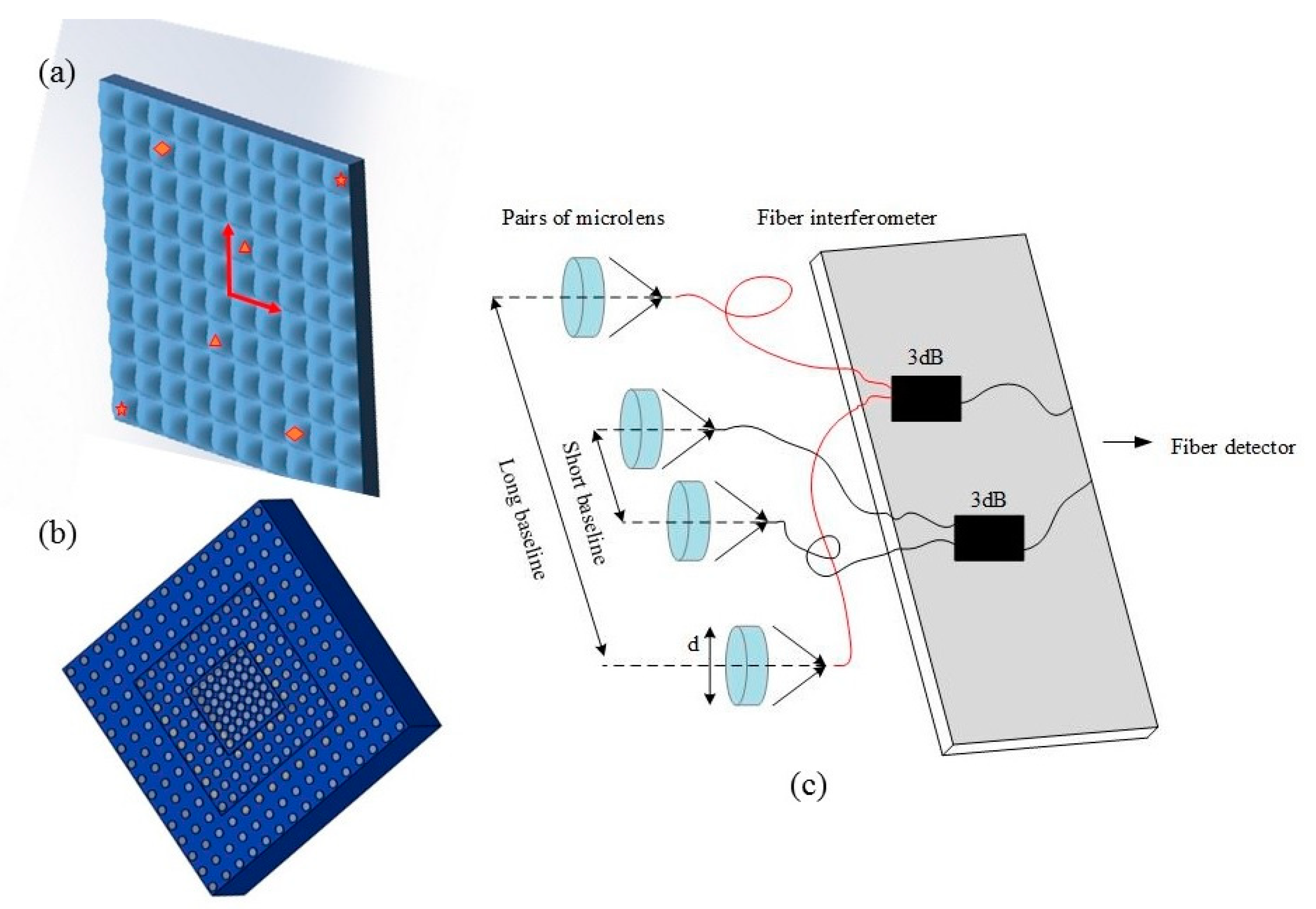
The structure of the electro-optical imaging system, which consists of a microlens array, fiber interferometer, and a processing module, is shown in Figure 1. The light information is collected and coupled into the fiber interferometer by the microlens array. Then, the interference fringes are detected and analyzed by the processing module. Finally, a computer generates an image based on the amplitude and phase information extracted from the interference fringes. Each fiber interferometer includes a pair of microlenses for measuring the spectrum of one baseline.

The spectral distribution measurement was determined by the arrangement and pairing of the microlenses. As shown in Figure 1a, the rectangular microlens array uses a centrally symmetric baseline pairing method (e.g., pentagram and pentagram, diamond and diamond, etc.). We also proposed a complex rectangular sub-aperture arrangement method to optimize the microlens-array arrangement (Figure 1b). The complex rectangular sub-aperture arrangement achieved different sampling intervals at high, intermediate, and low frequencies.

The performance of the fiber interferometer is closely related to the quality of interference fringes, whose core device is a 3-dB fiber coupler. Because achieving a fiber coupler coupling efficiency of 100% is difficult, the split ratio cannot be 1:1 [13]. Interference arm length differences of the fiber optic interferometer will also introduce additional phase differences, which will eventually affect the true reflection of the stripe contrast and phase.

3. Theory and Algorithm

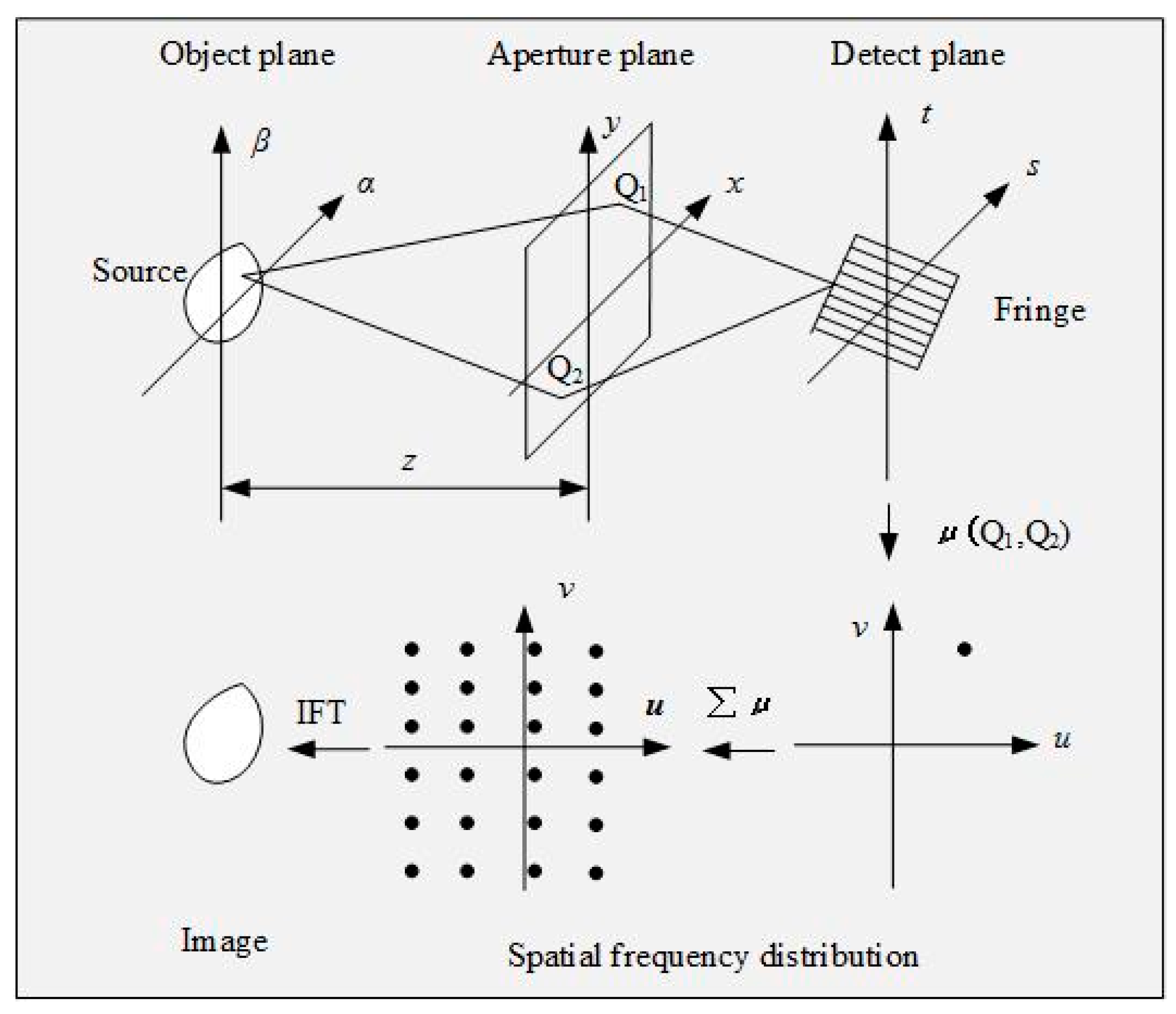
Figure 2 shows the principle and processes of the electro-optical imaging technology; they consist of four parts: interference between microlens pairs, calculation of complex degree of coherence according to fringes, spectral coverage, and image reconstruction.

Using the Van Cittert–Zernike theorem in partial coherence theory [8], this study analyzes the mutual intensity of a light field illuminated by an incoherent source and reaches an important conclusion: when the linearity of the source and observation area are much smaller than the distance between them, the complex coherence coefficient over the observation area is proportional to the normalized Fourier transform of the source intensity. According to the principle shown in Figure 2, the complex coherence coefficient between Q₁ and Q₂ in aperture planes can be expressed as [14]:

$$\mu \left(Q_1,Q_2\right)=\frac{{{\displaystyle \iint }}_{-\infty }^{+\infty }o\left(\alpha ,\beta \right)exp\left[-j\frac{2\pi }{\lambda z}\left(\left(x_2-x_1\right)\alpha +\left(y_2-y_1\right)\beta \right)\right]d\alpha d\beta }{{{\displaystyle \iint }}_{-\infty }^{+\infty }o\left(\alpha ,\beta \right)d\alpha d\beta }$$

(1)

$$\{\begin{array}{c}u=\frac{\Delta x}{\lambda z}=\frac{\left(x_2-x_1\right)}{\lambda z}\\ v=\frac{\Delta y}{\lambda z}=\frac{\left(y_2-y_1\right)}{\lambda z}\end{array}$$

(2)

According to Equation (2), the distance between the sub-apertures Q₁ and Q₂ in a pair is called the interferometer baseline, which is closely related to the spatial frequency $(u,v)$ of the detection scene. Therefore, we can optimally arrange the microlens array and use a better baseline-pairing method to realize spatial frequency coverage. Equations (1) and (2) provide a theoretical basis for interference imaging, which is different from the aberration imaging theory and the diffraction imaging principle.

The first step in reconstructing the image is to solve the complex coherence coefficient of a pair of lenses. According to the partial coherence theory, the complex coherence coefficient of two apertures on the observation plane can be determined by measuring the interference fringes. The second step is to change the interference baseline and repeat the first step to achieve spectral coverage. Finally, the solution result is substituted into the Equations (1) and (2), and the inverse intensity of the target scene is obtained by using the inverse Fourier transform. The detailed process and the simplified version of the program are shown in Algorithm 1.

Algorithm 1. Imaging process and reconstruction algorithm. Solving fringes and image reconstruction

1:  Initial(obj,aperture, …); 2:  for i,j = 1: (size(aperture))               //Step2: Change the interference baseline 3:    for s,t = 1: max max(size(obj))          //Step1: Solve one complex coherence coefficient 4:      Δphase = 2π/λ*d(s,t); 5:      I1 = Σ(1 + I0*cos(Δphase)); I2 = Σ(1 + I0*cos(Δphase + π/2));      //Interference fringe expression 6:      I3 = Σ(1 + I0*cos(Δphase + π)); I4 = Σ(1 + I0*cos(Δphase + 3π/2)); 7:    end 8:    absIM(i,j) = actan((I4 − I2)/(I1 − I3));              //Amplitude and phase 9:    angIM(i,j) = (I4 − I2)/2/sin(angIM); 10:  end 11:  IM = absIM*exp(angIM);

12:  im = fftshift(ifft2(IM));                  //Step3: Image reconstruction

If the interference fringe coordinate system is omitted, the fiber interference fringe intensity of any interference baseline can be expressed as [15]:

$$I=I_0\left(1+\left|\mu \right|\cos \left(\phi \right)\right)$$

(3)

In current interferometric measurements, the most commonly used phase calculation method is the four-step phase shift algorithm. This type of algorithm has extremely high measurement accuracy, anti-interference, and high calculation speed [16,17,18]. In this study, the visibility and phase of interference fringes are calculated by a four-step phase shift formula. The result can be expressed as [17,18]:

$$\{\begin{array}{c}{I}_1=I_0\left(1+\left|\mu \right|\cos \left(\phi \right)\right)\\ \begin{array}{c}{I}_2=I_0\left(1+\left|\mu \right|\cos \left(\phi +\pi /2\right)\right)\\ I_3=I_0\left(1+\left|\mu \right|\cos \left(\phi +\pi \right)\right)\\ I_4=I_0\left(1+\left|\mu \right|\cos \left(\phi +3\pi /2\right)\right)\end{array}\end{array}$$

(4)

$$\{\begin{array}{c}\phi ={\tan }^{-1}\left(\frac{I_4-I_2}{I_1-I_3}\right)\\ \left|\mu \right|=\frac{I_4-I_2}{2\sin \phi }\end{array}$$

(5)

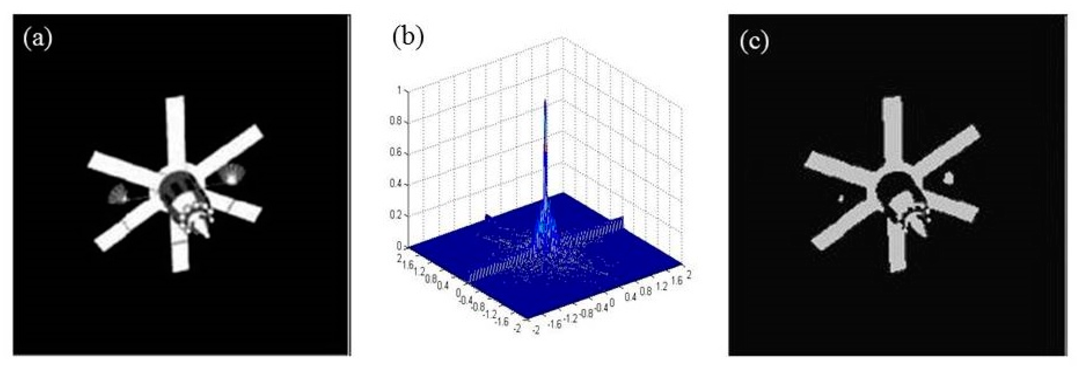
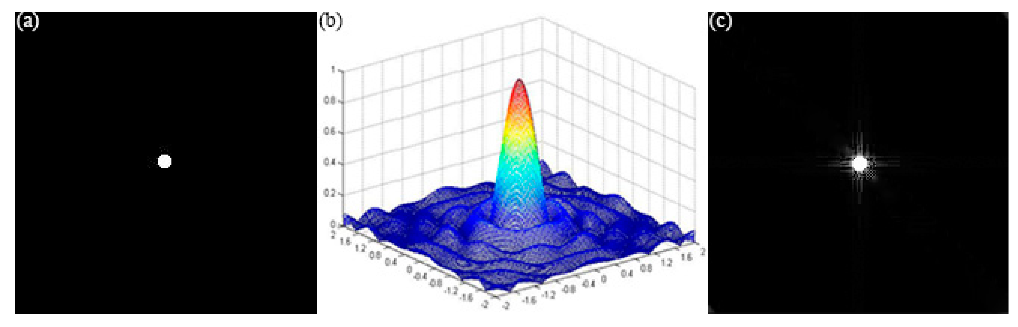
We adopt the parameters in

Table 1. Simulation parameters of the imaging system.

	Parameters	Symbol	Value
Object plane	Scene side length	D	30 m
	Number of samples	Nob	200 × 200
Aperture plane	Sampling interval	ΔuΔv	0.33 m−1
	Number of microlenses	Nap	200 × 200
	Diameter of microlens	r	1 mm
Image plane	Number of samples	Nim	1200 × 1200
System	Wavelength	λ	600 nm
	Object distance	z	105 m

to simulate a point source imaging process rectangular microlens array, and the results are shown in Figure 3. For the numerical simulation, we used a square-arranged microlens array and a centrally symmetric arrangement. Figure 3a presents the light intensity distribution of the target source. Figure 3b shows the detected spatial frequency distribution. Figure 3c shows the image obtained by an inverse Fourier transform. The results validate the imaging principle and simulation model.

4. Numerical Simulation of the Imaging System

According to the point-source imaging simulation, as compared with the target source (Figure 3a), the reconstructed image (Figure 3c) is obviously poor. Therefore, we perform further simulations by changing the system parameters in order to evaluate the imaging resolution and quality.

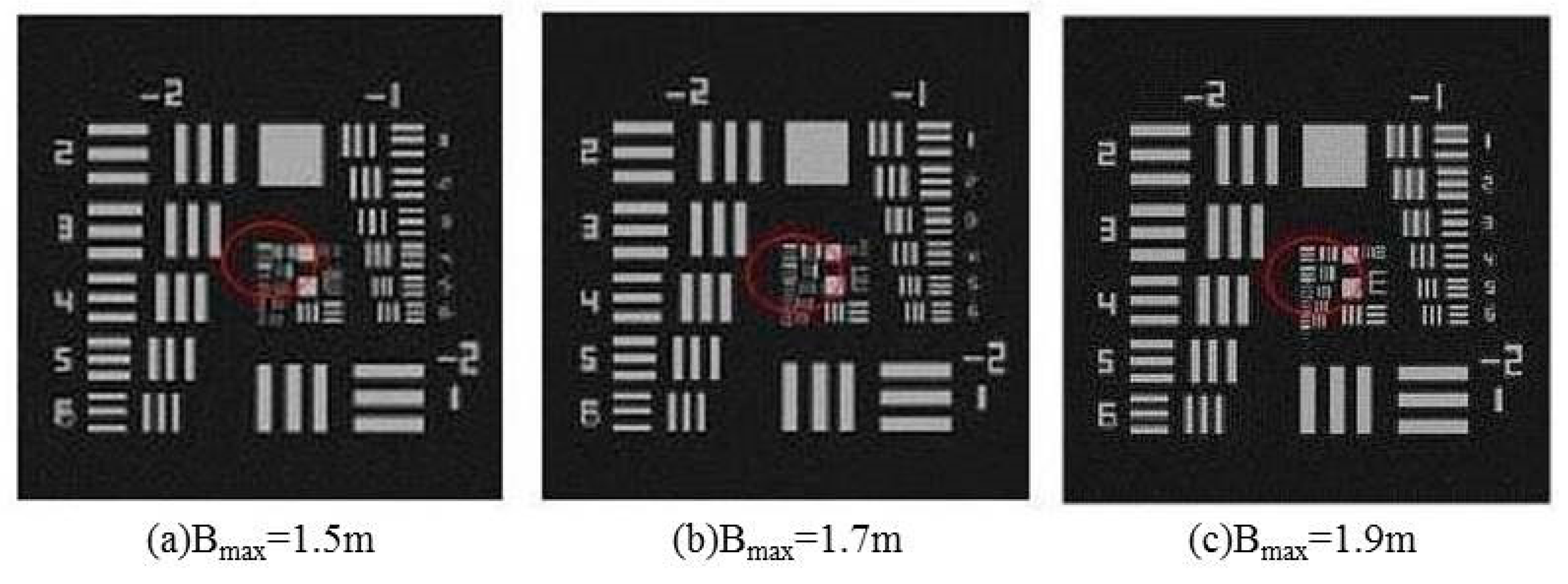
First, we only change N_ob, to simulate a resolution panel. With the same sampling interval, N_ob determines the maximum interference baseline length (B_max). According to imaging Equations (1) and (2), the larger the interference baseline length, the richer the high-frequency information contained, and the higher the imaging resolution. The imaging achieved by the system when the maximum baseline (B_max) is 1.5, 1.7, and 1.9 is shown in Figure 4a–c. It is obvious that the image resolution was up to the length of the maximum baseline. This result also provides a basis for improving the resolution of the imaging system.

The Nyquist sampling density affects the detected spatial frequency distribution. An extremely small sampling density can result in the loss of target information. In contrast, a high sampling density leads to information redundancy. However, the minimum sampling interval is limited to the sub-aperture size (r). Therefore, we have performed several repeated digital simulation experiments on the relationship between sampling density and imaging quality.

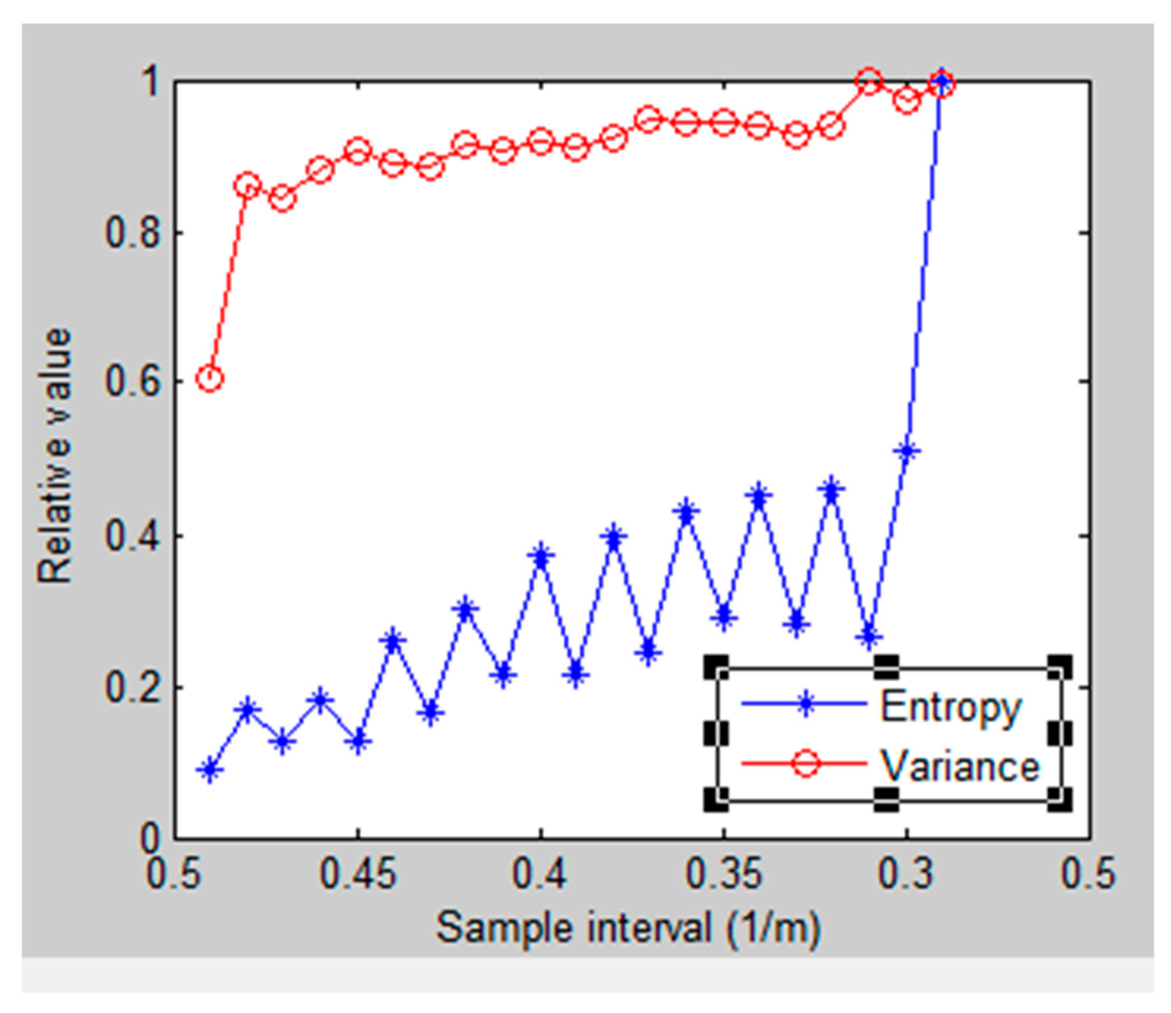
In this regard, we introduce a sharpness evaluation function to evaluate the image quality. The commonly used spatial domain functions for sharpness evaluation are listed in the literature, among which the spatial domain functions represented by the variance function and the entropy function perform better [19]. We use two imaging quality evaluation methods based on gray variance and entropy function.

We use the resolution board as the source target and change the sampling interval. The relationship between the value of the gray-scale variance and entropy and the sampling interval is shown in Figure 5. We see that the imaging quality can be improved by increasing the sampling density, although these two evaluation functions are not sensitive to small local changes. In addition, the imaging system has no oversampling when the minimum sampling density is equal to the sub-aperture size (△u = 0.33). Thereafter, we used a photograph of an airplane (Figure 6) as the original target to perform the same simulation. Based on the results (Figure 7), we draw the same conclusion, although we compare the image quality visually in this case.

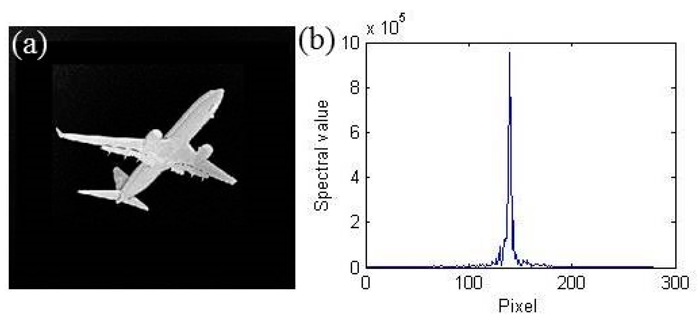
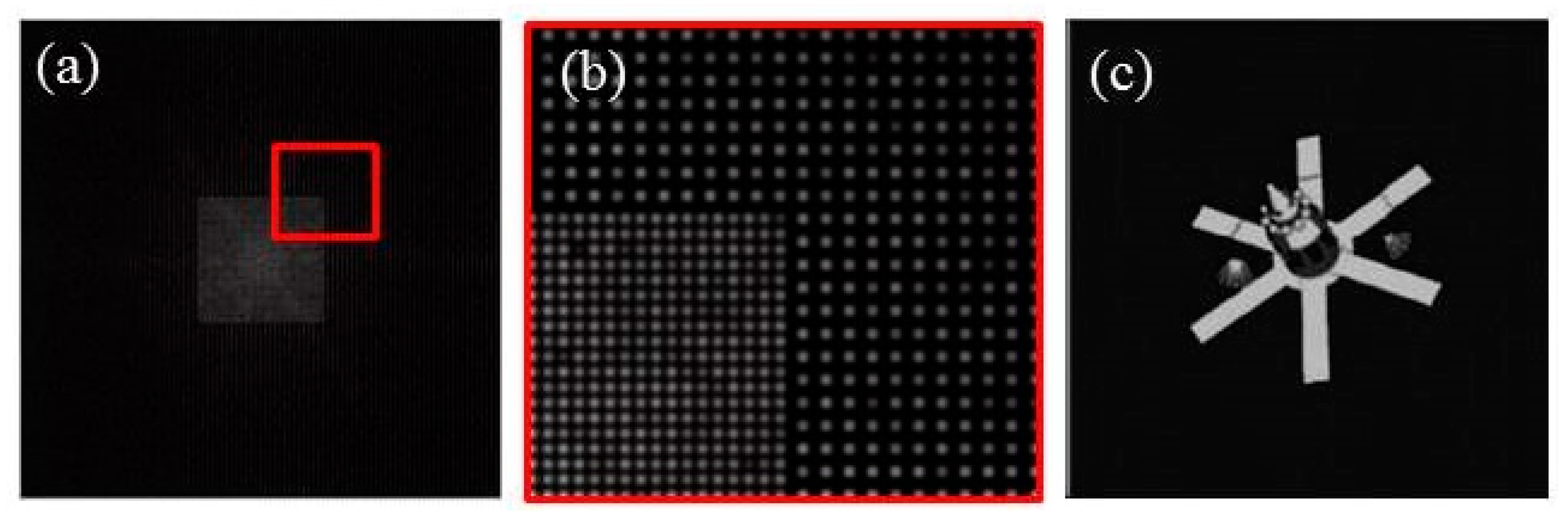
It is well known that different sources have different frequency information. For some sources, the frequency information was concentrated in the low-frequency part; therefore, the sampling density was increased to obtain a high-quality image. This resulted in a corresponding increase in system complexity. A satellite was used as the detection target; from the simulation results (Figure 8), it can be seen that the spectrum information of the satellite image is concentrated in the low-frequency part. We attempted to improve the image quality without increasing the number of microlenses, i.e., the complexity of the system. Then, the complex rectangular sub-aperture arrangement method was adopted to adjust the sampling density at high and low frequencies separately.

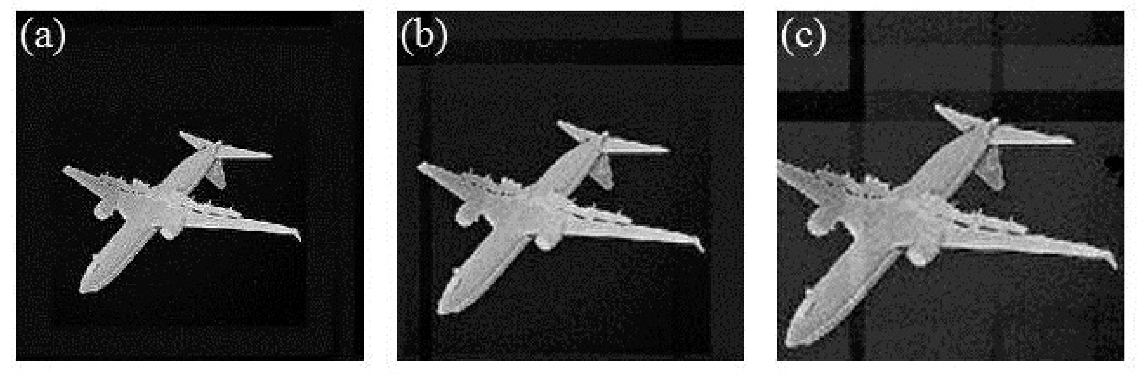
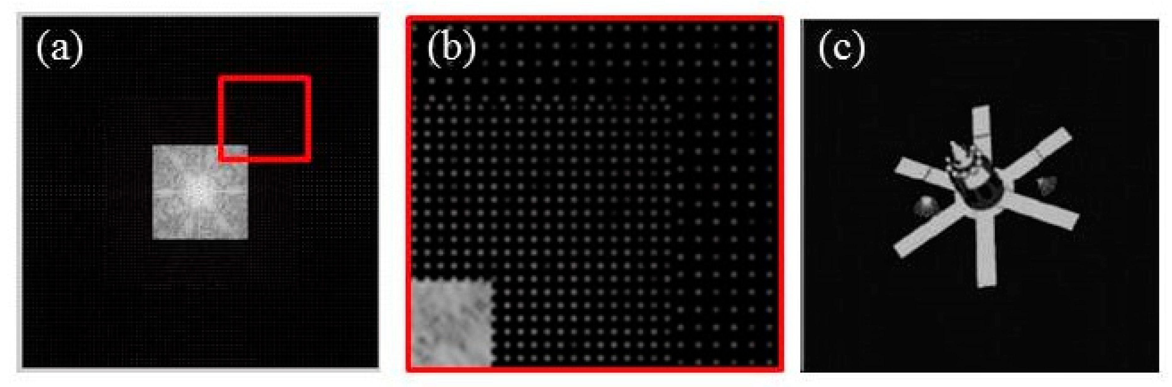
In the results presented in Figure 8, the sampling interval is uniformly set to △u = 0.33. In Figure 9, the sampling spectrum is divided into two parts, a high frequency and a low frequency, and the sampling intervals are respectively set to △u1 = 0.19, △u2 = 0.38. Similarly, the sampling intervals are set to △u1 = 0.33, △u2 = 0.66, △u3 = 1.3 in Figure 10. The above settings ensure that the number of microlenses used in the three sampling modes is nearly equal.

The simulation results are shown in Figure 8, Figure 9 and Figure 10. Visual comparison shows no difference in image quality. This shows that the complex rectangular sub-aperture arrangement method proposed in this paper is feasible. We use variance and entropy to evaluate the subtle differences between the images. The results are presented in

Table 2. Imaging process and reconstruction algorithm.

The Number of Complex Arrangements	Parameter	Variance	Entropy
1	△u = 0.33, N = 200	1.5087 × 108	3.7735
2	△u1 = 0.66, △u2 = 0.99, N = 200	1.4983 × 108	3.7765
3	△u1 = 0.33, △u2 = 0.66, u3 = 1.3, N = 200	1.6364 × 108	3.8652

, which proves that higher-quality images could be obtained with the same number of microlenses.

5. Conclusions

This paper proposes a cutting-edge electro-optical imaging technology based on a microlens array and fiber interferometer, a centrally symmetric baseline pairing method, and a complex rectangular sub-aperture arrangement method. We then briefly analyze the theoretical basis of the imaging system and the method of analyzing the fringes. Finally, the imaging system was verified by digital simulation.

The main conclusions are as follows: (1) the resolution of the imaging system can only be improved by increasing the maximum baseline length; (2) increasing the Nyquist sampling density increases the density of the spatial frequency points and improves the imaging quality; (3) by adopting the complex rectangular sub-aperture arrangement, better image quality can be obtained without increasing the complexity of the imaging system.